Sage Journals: Discover world-class research

Abstract

Using a factor-augmented vector auto-regression model and quarterly U.S. data from 1960 to 2019, I estimate the effect of changes in government spending on key economic variables such as output and household consumption. Unlike previous studies which show a positive effect of government spending on output, I find that adding factors to the VAR model erases the positive effect of spending and reveals a small but statistically significant negative response in output and consumption. Other instances of crowding out include increases in interest rates and price levels and decreases in investment and net exports.

Keywords

Government spending economic output fiscal policy stimulus crowding out factor-augmented vector auto-regression (FAVAR)

Introduction

Can government spending be used to stimulate the U.S. economy? There are few questions in the economics discipline that have sparked as much interest among researchers, policymakers, and the public at large. In the United States, severe recessions such as those in 2008 and 2020 have sustained interest in the use of fiscal policy as a tool for boosting output and shortening the duration of economic downturns. If government spending can spur an increase in output, then fiscal stimulus may be an effective way to raise economic welfare and accelerate recovery.

The standard neoclassical economic model predicts that an increase in unproductive government spending would not have a positive effect on output. On the other hand, a simple Keynesian model, which includes the assumption that prices are sticky, allows for the possibility that government spending can cause output to increase. Some new Keynesian models even show that government spending can cause household consumption expenditures to increase (e.g., Gali, Lopez-Salido and Vallés 2007).

Although the empirical literature contains evidence supporting both perspectives, a consensus has emerged in the vector autoregression (VAR) literature which asserts that while government spending does crowd out investment spending, it has a positive effect on output and consumption. However, this literature consistently suffers from a few limitations. First, due to a limited quantity of data, VAR models in the macroeconomics literature contain very few variables and could therefore result in estimates that do not reflect important economic activity. Second, they do not adequately account for the expectations of agents in the economy. Assuming that households and firms are rational and well-informed of current events, they could respond to news of a change in spending well before the spending shock is recorded.

To address these issues, I estimate a structural factor-augmented vector autoregression (FAVAR), augmented with factors derived via principal components analysis from a dataset of 216 macroeconomic variables covering a broad range of categories. The factors condense information from the full dataset, enhancing the VAR's representation of the broader economy. My findings indicate that the initial effects of government spending on output and consumption are negative across all five-factor specifications. Although the magnitude and persistence of these effects vary by spending type and model variant, the immediate contractionary response is robust. The only exception to this pattern is government investment spending, which initially contracts output before ultimately yielding a positive effect.

This paper contributes to the literature in three main ways. First, it estimates a structural FAVAR using a broader set of macroeconomic variables than most prior studies, allowing for a richer information set and more credible identification of fiscal shocks. Unlike much of the previous FAVAR literature, which relies on sign restrictions, this paper identifies shocks using a recursive (Cholesky) decomposition. This approach permits contractionary responses to government spending shocks that sign restrictions would otherwise rule out by assumption. Second, it uses a longer time series than many comparable analyses, which helps stabilize the estimates and test whether earlier findings hold over time. Third, it disaggregates government spending into multiple categories and finds that these distinctions matter substantially for the results. In particular, government investment spending exhibits substantially different dynamics from other forms of spending. Together, these innovations produce results that challenge the prevailing view in the VAR literature, suggesting that crowding out effects may be stronger and more immediate than previously recognized.

To construct the factors used in the FAVAR, I use 216 quarterly macroeconomic time series from the Federal Reserve Bank of St. Louis's FRED-QD database. These series span a wide array of U.S. economic indicators, including national income and product accounts, labor markets, housing, prices, interest rates, financial markets, and balance sheets. This breadth ensures that the extracted factors capture a wide range of information relevant to the dynamics of fiscal shocks.

This paper is organized as follows: Section 2 reviews the related literature; Section 3 describes the empirical model; Section 4 outlines the data; Section 5 presents the results; Section 6 presents the robustness specifications; and Section 7 concludes.

Literature Review

While there is considerable debate about the size of the output multiplier, the empirical literature generally agrees that it is positive. However, empirical research on the effects of government spending shocks on private consumption is mixed. The literature is divided not only on the size of the consumption multiplier, but also on the sign.

Ramey and Shapiro (1998) addressed the question using a narrative approach by including a dummy variable for periods of large U.S. military buildups and found a statistically significant decline in private consumption following a government spending shock.

Blanchard and Perotti (2002) examined the dynamic effects of shocks in government spending in the United States. They argued that government spending does not respond to output or taxes within the same quarter and found empirical support for this assumption. This allowed them to identify government spending shocks with government spending ordered first in the Cholesky decomposition. They found that private consumption tends to rise after positive government spending shocks. Other studies have also used the VAR approach and found that there was a crowding-in effect of private consumption following a government spending shock (e.g., Fatas and Mihov (2003); and Mountford and Uhlig (2009)).

More recently, Ramey (2011a) explored this very issue by comparing the strengths of the VAR approach to her narrative approach with regard to their ability to explain the effect of government spending on consumption. She argued that the VAR approach suffers from key limitations in identifying the relationship between government spending and consumption. Central to her argument was that the VAR method did not account for the public's expectations. This is especially important in the case of identifying fiscal shocks because, unlike monetary policy, fiscal policy features decision and implementation lags which allow the public to adjust behavior in anticipation of fiscal policy changes. Ramey (2011a) concluded that the VAR approach may be biased due to this timing issue. Additionally, Leeper, Walker and Yang (2010) called this a “fiscal foresight” problem and analyzed its econometric implications. They argued that the difference between the set of information observed by the private agents and the one observed by the econometrician can be quite significant, and it could easily bias estimates of the effects of fiscal shocks.

These critiques can be interpreted as a limited information problem. The sparse information set typically used in the standard VAR models leads to fiscal policy shocks that do not account for the public's expectations. Notably, studies by Tenhofen and Wolff (2007), Mountford and Uhlig (2009), and Auerbach and Gorodnichenko (2012) have attempted to address this issue. These works highlight the importance of capturing expectations in empirical models and the role of different types of government spending in influencing fiscal multipliers. Despite these attempts, limitations associated with the sparse information set in standard VAR models persist, suggesting the need for an alternative approach.

In this paper, I investigate one solution to this limited information problem, which combines the standard VAR model with a factor model. The resulting model, which is particularly appealing in this case, is the factor augmented vector autoregression (FAVAR) of Bernanke, Boivin and Eliasz (2005). The FAVAR method implements a two-stage approach. In the first stage, principal component analysis is used to extract a relatively small number of factors from a large set of “informational” variables. Such an informational dataset includes a wide range of economic variables that capture unanticipated government spending shocks. In the second stage, the factors are included in the VAR. This method incorporates rich information into the VAR while preserving degrees of freedom. Using a FAVAR to estimate the effects of government spending shocks addresses the critiques made in Ramey (2011a) in a more systematic manner.

This study also contributes to the broader fiscal multiplier literature. While many papers in that literature estimate multipliers greater than one, these estimates often rely on identifying assumptions or data limitations that lean toward expansionary results. I find that output and consumption tend to decline modestly after spending shocks, suggesting that crowding-out effects may be more common than previously thought. These findings underscore the importance of model design and identification strategy when assessing fiscal policy effects.

While other studies have used factor-based approaches, they rely on significantly smaller datasets, adopt identification strategies that may influence the results, or focus on a narrow subset of government spending. Gupta, Kabundi and Ziramba (2010) use a FAVAR with 116 variables to evaluate the effect of defense spending shocks and find a generally positive effect on output that is only statistically significant for two quarters. Similarly, Fragetta and Gasteiger (2014) estimate a FAVAR using 62 variables and three factors. They find large fiscal multipliers in excess of two. In addition, Forni and Gambetti (2010) estimate a structural, large-dimensional, dynamic factor model using 106 variables. They find that the impact multiplier of government spending on output is 1.7 with a long-run multiplier of 0.6. They also find that spending causes increases in consumption, like in the previous literature, and unlike earlier studies, find that investment increases. Their use of sign restrictions precludes the possibility of contractionary responses, making negative relationships unlikely by construction.

Laumer (2020) applies a Bayesian FAVAR with over 200 variables and also finds that government spending increases output and consumption. However, the identification strategy used in that study defines spending shocks as those that raise output, employment, prices, tax receipts, the deficit, and government spending. Although the response of consumption is formally left unrestricted, the definition of a shock as one that causes widespread expansion means that contractionary responses are unlikely to emerge from the data. In contrast, my identification strategy does not impose restrictions on macroeconomic outcomes and instead allows the data to determine whether government spending is expansionary or contractionary. This distinction likely accounts for the divergence in results.

More broadly, Fry and Pagan (2011) warn that sign-restricted SVARs, widely adopted in recent fiscal studies, tend to report overly precise impulse response functions by failing to fully account for uncertainty. They determine that the reported bands reflect variation across admissible sign patterns rather than true statistical uncertainty. Nonetheless, many of the aforementioned studies adopt sign-restricted SVARs to estimate the effect of government spending on output and present impulse responses as if they were precisely identified. While these models can identify sets of shocks consistent with assumed sign restrictions, they do not recover a unique structural model or the scale of the shocks. As a result, their apparent precision may be misleading, offering limited guidance for quantifying the true magnitude of fiscal multipliers.

Finally, Kim (2019) estimates a FAVAR model using 167 variables to measure the impact of shocks in government consumption and investment in Korea and finds evidence of crowding out via the current account rather than through a reduction in private consumption and investment.

Only a handful of papers attempt to assess the differential effects of disaggregated government spending categories. Marattin and Salotti (2011) estimate a structural VAR for EU countries and find heterogeneous effects across spending types such as public investment and compensation of employees. More recently, van Gemert, Lieb and Treibich (2022) uses a local projection method on Dutch data and similarly reports differences across components like defense and public consumption. However, these studies use relatively limited information sets. In contrast, my study combines a broad U.S. data panel with a FAVAR framework and disaggregates government spending into a wider set of categories. This allows for a more comprehensive assessment of which spending types are most likely to generate crowding out or expansion.

This paper differs from previous studies in several crucial ways: utilization of a larger informational dataset, a greater number of factors, which ensures informational sufficiency, an identification strategy that permits the effects of fiscal policy to be either expansionary or contractionary, and closer adherence to the FAVAR methodology outlined by Bernanke, Boivin and Eliasz (2005). Finally, rather than evaluating one or two spending categories, I systematically examine a broad variety of spending types, generating detailed insights into how different components of government spending affect output, private consumption, and investment.

Model

The FAVAR

This paper uses a factor-augmented vector autoregression model that is adapted from the one used by Bernanke, Boivin and Eliasz (2005) for the purpose of studying fiscal policy. The model consists of a traditional structural VAR that includes a number of factors computed with principal components analysis.

Consider a traditional structural VAR with an M × 1 vector Y_t whose elements reflect a few observable variables that drive the dynamics of the economy. The standard approach in the literature is to proceed as in Blanchard and Perotti (2002) and estimate a structural VAR solely with data from Y_t.

However, it is possible that there exists a wide range of additional economic information that pertains to the dynamics of the variables contained in Y_t. Suppose there is a K × 1 vector F_t of factors that summarize the additional information, where K is “small”. The following system can then represent the joint dynamics of F_t and Y_t:

(\begin{matrix} F_{t} \\ Y_{t} \end{matrix}) = Φ (L) (\begin{matrix} F_{t - 1} \\ Y_{t - 1} \end{matrix}) + v_{t}

(1)

where Φ(L) represents a conformable lag polynomial of finite order d. The error term, v_t, has a zero mean value and a covariance matrix Q.

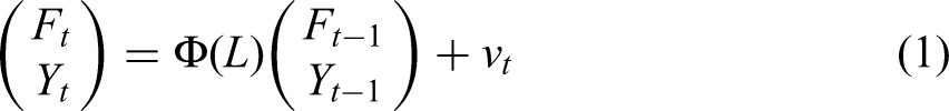
Equation 1 is a VAR in the observable variables and the factors. This structure is referred to as a factor-augmented VAR. It is important to note that if equation 1 is the true model, then estimating a VAR that excludes F_t can result in biased estimates. One major advantage of this method is that the standard VAR model is nested within the FAVAR model. Therefore, the FAVAR maintains the same interpretation that would be made with the original VAR while also addressing the possible limited information problem discussed earlier.

Identification

Because the reduced-form residuals lack structural interpretation, identifying the structural shocks to taxation and government spending, which are mutually uncorrelated, is of paramount importance. One of the main differences between this paper and Forni and Gambetti (2014) is the identification strategy. They identify government spending shocks through the application of sign restrictions, defining an expansionary shock as one that has a positive effect on various variables, including government spending and GDP, after six months. Sign restrictions of this nature have received some criticism in recent years. For example, Baumeister and Hamilton (2015) examine the ways in which the imposed priors can influence the posterior distribution. This approach imposes a certain relationship between government spending and key economic variables, and is likely ill-suited for assessing whether government spending has a contractionary effect on output.

This paper follows Bernanke, Boivin and Eliasz (2005) in using a Choleski decomposition, with F ordered before Y for identification. This allows shocks identified in Y to incorporate information from the broader dataset represented by F. The strategy of placing F first in the Cholesky decomposition is further justified in the estimation subsection.

The variables included in Y are ordered as follows: government spending, net taxation, gross domestic product, and consumption expenditures. Therefore, the identification strategy relies on the assumption that government spending is not intratemporally correlated with any other variables contained in Y within one quarter which is consistent with the findings of Blanchard and Perotti (2002). As they point out, the main concern is the ordering of government spending and taxation as it is not obvious which variable has an immediate effect on the other. Similar to their paper, I address this by estimating the five-factor model where government spending and taxation are swapped. There was no discernible difference between the two orderings, so I conclude, as Blanchard and Perotti (2002) did, that the results are not sensitive to this choice in the identification strategy.

Estimation

The system in equation 1 cannot be estimated using standard regression methods because the vector F_t is unobservable. To extract these factors, let X_t be an N × 1 vector where N is considered large; X_t represents the large set of “informational” variables discussed earlier. Because X_t is too large to include in the VAR directly, its information is summarized by the K factors in F_t. In order to infer the values for F_t, I assume that X_t is related to F_t and Y_t according to the following equation:

X_{t} = Λ^{f} F_{t} + Λ^{y} Y_{t} + e_{t}

(2)

where Λ ^f is the N × K matrix of factor loadings, Λ ^y is N × M, and e_t is an N × 1 vector of mean-zero error terms which are assumed to be weakly correlated. Equation 2 shows how the observed data X_t is related to the latent factors and VAR variables, enabling estimation of F_t from the larger informational dataset.

Equations 1 and 2 are estimated using the two-step procedure outlined by Bernanke, Boivin and Eliasz (2005). Since F_t is assumed to be related to the variables in both X_t and Y_t, the first step involves estimating Ĉt, the principal components of the entire data set, which includes X_t and Y_t. The resulting factors, according to Stock and Watson (2002), result in coverage that spans the space covered by F_t and Y_t. Since the factors will be ordered first in the Cholesky decomposition, some identifying assumptions must be made to ensure that the factors are not contemporaneously responsive to shocks in the Y variables. To account for this, I distinguish between slow-moving and fast-moving variables. The variables are categorized as slow or fast similarly to Bernanke, Boivin and Eliasz (2005). See the appendix and accompanying tables for more information on how each variable was categorized. Then, “slow-moving” factors, F^s are estimated using the principal components of the slow variables. To retrieve the factors for use in the VAR, I estimate the following linear regression,

\hat{C_{t}} = b_{F} {\hat{F}}_{t}^{s} + b_{Y} Y_{t} + u_{t}

(3)

and

{\hat{F}}_{t}

is calculated with Ĉt −

{\hat{b}}_{Y}

Y_t. The factors,

{\hat{F}}_{t}

, represent the information from the entire data set, X_t, but not including the space already covered by Y_t. Since equation 3 includes only the slow factors as dependent variables,

{\hat{F}}_{t}

is not correlated contemporaneously with the variables in Y_t which justifies the identifying assumption of placing the factors first in the Cholesky decomposition. The VAR described in equation 1 is then estimated using

{\hat{F}}_{t}

in place of F_t.

Informational Sufficiency

The paper includes results from the model using zero, three and five latent factors to illustrate the effect of including more information to a model similar to that of Blanchard and Perotti (2002). However, five latent factors are the minimum number of factors required in order to achieve informational sufficiency. This was determined by implementing the test suggested by Forni and Gambetti (2014) which involves estimating the VAR model with a certain number of factors and determining whether an additional factor Granger causes the previously included variables in the VAR. Informational sufficiency is achieved when an additional factor no longer Granger causes the other variables in the VAR. In this case, the model lacks informational sufficiency until the fifth factor is added so that the p-value associated with the Granger causality test of a sixth factor is 0.1171, indicating it does not significantly Granger-cause the VAR variables. This validates that the information set used in the five-factor model is rich enough to capture the relevant macroeconomic dynamics.

Data

The data used in this paper are collected quarterly and cover the years 1960–2019. Table 3 in the appendix lists the variables used to compute government spending and net taxation, along with their FRED mnemonics. Following Blanchard and Perotti (2002), I compute government spending as the sum of federal defense expenditures, federal nondefense expenditures, and state and local expenditures, which include both consumption and investment. Net taxation is calculated as total federal, state, and local receipts minus the sum of government interest payments and transfer payments across all levels of government. I obtained the government spending and net taxation data from the Bureau of Economic Analysis.

The dataset ends in 2019Q4, deliberately excluding the COVID-19 pandemic due to the unprecedented nature of the associated fiscal responses and macroeconomic conditions. As emphasized by Faria-e-Castro (2021) and Deb et al. (2024), pandemic-era fiscal policy differed substantially in scale, composition, and transmission mechanisms from historical norms. Including these quarters would likely introduce structural breaks or nonlinearities that confound the interpretation of historical patterns. Future work could examine whether the results identified here extend to that episode using methods tailored to extreme interventions.

I derived the factors in the empirical model from the dataset obtained from FRED-QD: a quarterly data series offered by the Federal Reserve Economic Database. I used 216 variables from this database, which covers a broad range of relevant macroeconomic categories including: national income and product accounts, industrial production, employment, housing, inventories, prices, earnings, interest rates, money, household balance sheets, exchange rates, financial markets, and firm balance sheets. The dataset also includes necessary transformations for each variable to ensure stationarity. These data were gathered from a range of sources such as the U.S. Bureau of Economic Analysis, U.S. Bureau of Labor Statistics, Board of Governors of the Federal Reserve System, National Bureau of Economic Research, U.S. Census Bureau, Dow Jones, and Moody's Analytics. This dataset is well-suited to this study because of its extensive coverage of the U.S. economy. McCracken and Ng (2020) found that factors extracted from this database can significantly increase the ability of models to accurately create forecasts relative to VARs that lack the factors from this data.

Tables 4–17 in the appendix summarize the data obtained from FRED-QD. Each table entry includes the series description, FRED mnemonic, and transformation code. The transformation codes are: (1) no transformation; (2) Δx_t; (5) Δlog(x_t); (6) Δ²log(x_t); (7) x_t/x_t₋₁−1. Variables represented in dollar values are adjusted from nominal to real values using the GDP deflator.

Results

Impulse Response Functions

This section presents results from the estimated model and several alternative specifications. First, the model is estimated with no latent factors included, resulting in a traditional structural VAR akin to Blanchard and Perotti (2002). Then, I estimate the model using three and five factors. The five-factor model serves as the baseline because it achieves informational sufficiency and is suggested by the Akaike information criterion.

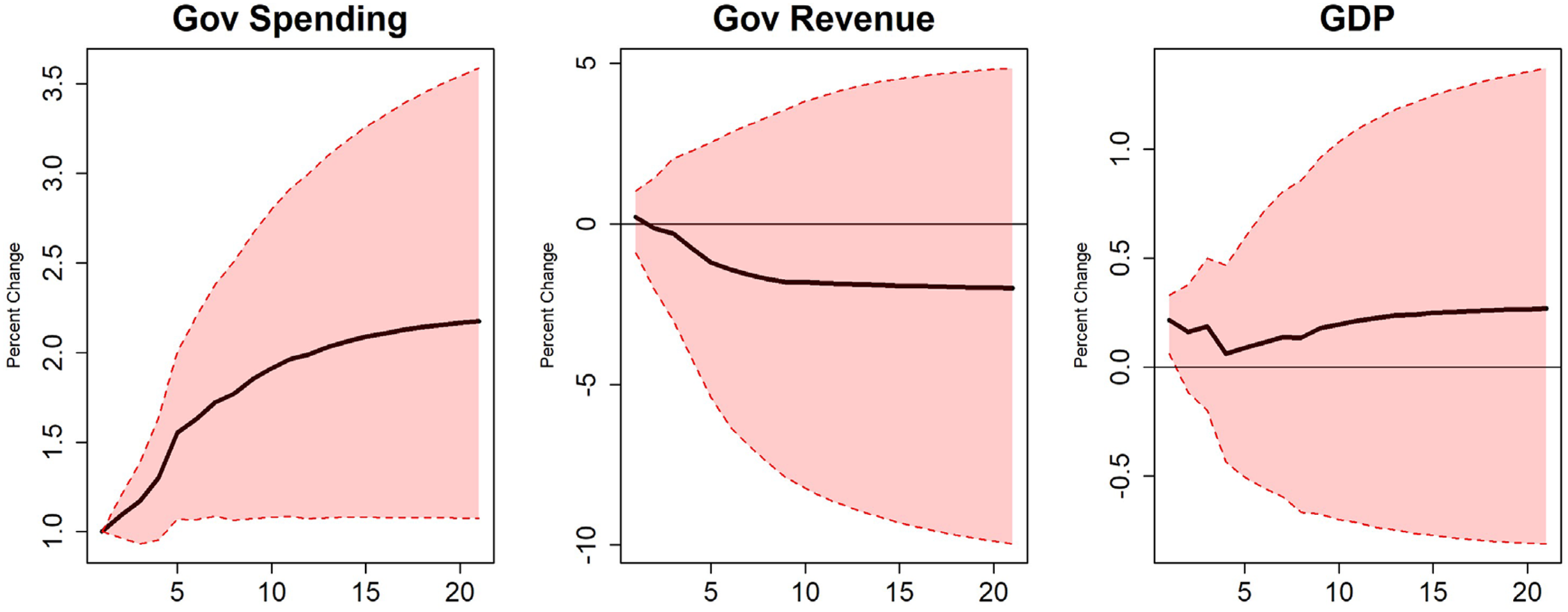
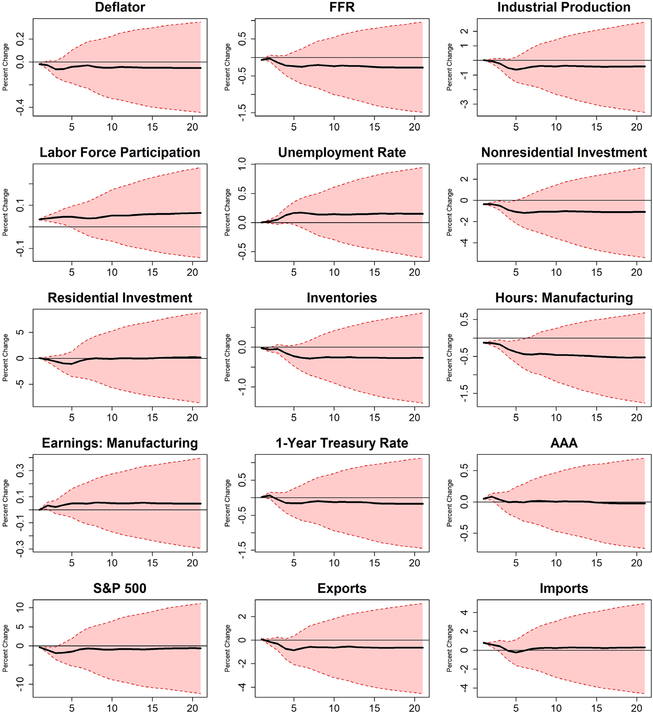
For each specification, I compute impulse response functions (IRFs) for 20 periods in which there is a 1% exogenous shock to government spending in the first period. Each result includes graphs showing the cumulative percent change in select variables where the solid black line reflects the estimated impact and the dotted red lines contain the 90% confidence interval for the estimate. Confidence intervals are computed using the Monte Carlo bootstrap procedure outlined by Bernanke, Boivin and Eliasz (2005).

The informational data set contains numerous variables which could have interesting interactions with government spending. While none of these variables are explicitly included in the VAR specification, their impulse response functions can be retrieved from the effects on the factors which are included in the model. Following Bernanke, Boivin and Eliasz (2005), I use this procedure to run a linear regression for each informational variable, with each informational variable treated as the dependent variable and the VAR variables as the independent variables. The regression coefficients are combined with the IRFs from the explicitly modeled VAR variables to calculate the estimated impact on the informational variables of interest.

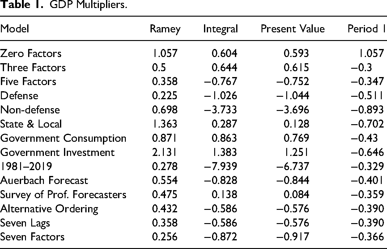
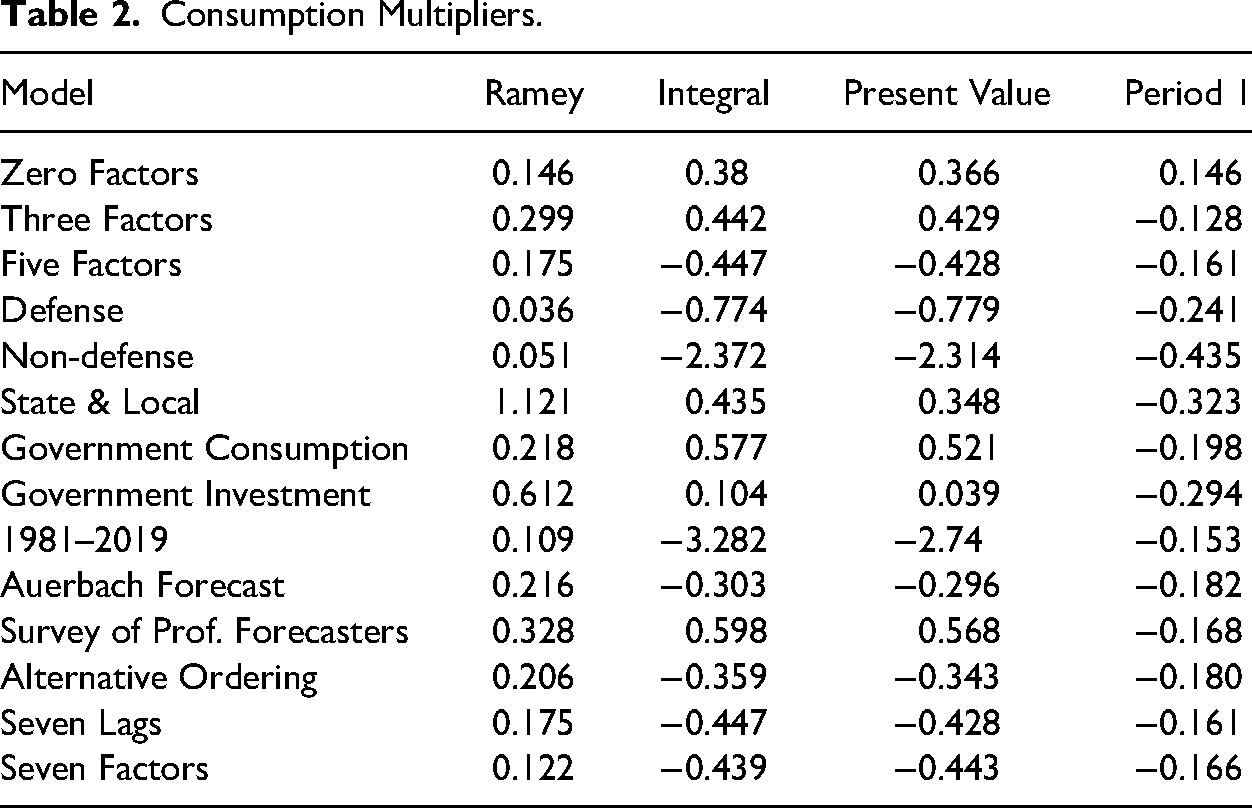
In addition to the IRF graphs, I compute four types of government spending multipliers for output and consumption, each measuring the effect of a 1% exogenous increase in spending. The initial multiplier reports the impact in period 1 and is calculated as the ratio of the output (or consumption) response to the period-1 change in spending, scaled by the average ratio of output (or consumption) to government spending. The peak multiplier, following Ramey (2011a), is the maximum value of this ratio over the 20-period horizon. The cumulative multiplier sums the output responses and divides by the sum of the spending responses, again scaled by the output-to-spending ratio; this measures the total effect over the horizon. The present value multiplier discounts each period's responses using a quarterly real interest rate of 1.03%, corresponding to a 4.2% annual rate based on 1-year Treasury yields, before computing the same output-to-spending (or consumption-to-spending) ratio. These four multipliers are reported for output in Table 1 and for consumption in Table 2.

Table 1.

GDP Multipliers.

Model	Ramey	Integral	Present Value	Period 1
Zero Factors	1.057	0.604	0.593	1.057
Three Factors	0.5	0.644	0.615	−0.3
Five Factors	0.358	−0.767	−0.752	−0.347
Defense	0.225	−1.026	−1.044	−0.511
Non-defense	0.698	−3.733	−3.696	−0.893
State & Local	1.363	0.287	0.128	−0.702
Government Consumption	0.871	0.863	0.769	−0.43
Government Investment	2.131	1.383	1.251	−0.646
1981–2019	0.278	−7.939	−6.737	−0.329
Auerbach Forecast	0.554	−0.828	−0.844	−0.401
Survey of Prof. Forecasters	0.475	0.138	0.084	−0.359
Alternative Ordering	0.432	−0.586	−0.576	−0.390
Seven Lags	0.358	−0.586	−0.576	−0.390
Seven Factors	0.256	−0.872	−0.917	−0.366

Table 2.

Consumption Multipliers.

Model	Ramey	Integral	Present Value	Period 1
Zero Factors	0.146	0.38	0.366	0.146
Three Factors	0.299	0.442	0.429	−0.128
Five Factors	0.175	−0.447	−0.428	−0.161
Defense	0.036	−0.774	−0.779	−0.241
Non-defense	0.051	−2.372	−2.314	−0.435
State & Local	1.121	0.435	0.348	−0.323
Government Consumption	0.218	0.577	0.521	−0.198
Government Investment	0.612	0.104	0.039	−0.294
1981–2019	0.109	−3.282	−2.74	−0.153
Auerbach Forecast	0.216	−0.303	−0.296	−0.182
Survey of Prof. Forecasters	0.328	0.598	0.568	−0.168
Alternative Ordering	0.206	−0.359	−0.343	−0.180
Seven Lags	0.175	−0.447	−0.428	−0.161
Seven Factors	0.122	−0.439	−0.443	−0.166

Given the large number of estimated specifications, I focus the discussion on three core scenarios: (1) total government expenditures, (2) a comparison of defense versus nondefense spending, and (3) government investment. These cases are emphasized because they most directly engage with central debates in the fiscal multiplier literature, particularly with respect to shock exogeneity, fiscal foresight, and heterogeneous output responses. The remaining specifications, such as state and local spending or government consumption, are summarized more briefly.

Zero Latent Factors

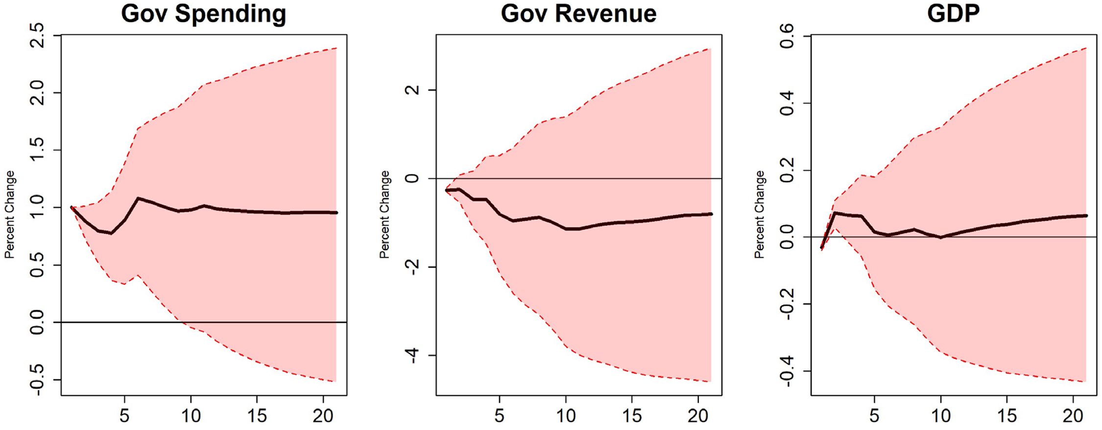
This subsection describes the results from estimating the model with no factors included. This results in a traditional structural VAR. The purpose of this exercise is to demonstrate that the model in this paper achieves results that are quite similar to those in Blanchard and Perotti (2002) when none of the information from the larger data set is present. Figure 1 summarizes the results from the computation of the IRF for this specification.

Figure 1.

Zero factors.

The most important result is that a 1% increase in government spending results in a large and statistically significant increase in output. This results in a peak multiplier of 1.057 which is also the multiplier in period 1. In addition, while the response to consumption is not statistically significant, the effect is positive with a peak consumption multiplier of 0.146 suggesting that government spending may have a “crowding in” effect on both consumption and output. These results are consistent with those found by Blanchard and Perotti (2002) who estimated a spending multiplier on output between 0.9 and 1.29 and a positive effect on consumption. Interestingly, the estimated impulse responses in this zero-factor model are short-lived, with GDP effects dissipating within a few quarters. This pattern is not unusual. Blanchard and Perotti (2002) report similarly short-lived effects under structural timing assumptions for non-defense spending. Since the zero-factor model here uses aggregate spending and mimics a traditional SVAR specification, the resemblance is informative. It suggests that short-lived responses may arise not from model misspecification, but from identification strategy and spending composition.

Three Latent Factors

This specification estimates the model with three factors included, with this number chosen based on the efficiency criteria offered by Bai and Ng (2002). Figures 2–4 summarize the results from this specification.

Figure 2.

Three factors part 1.

Figure 3.

Three factors part 2.

Figure 4.

Three factors part 3.

Including the information from the broader data set via the latent factors has a substantial effect on the results. The cumulative effect of government spending on output is still positive but greatly reduced with a peak output multiplier of 0.5 which is less than half the peak multiplier without factors. The change to output is also no longer statistically significant during any period. While total consumption remains unaffected, durable consumption declines significantly.

There are suggestive signs that government spending may crowd out private activity. Nonresidential investment and manufacturing earnings decline modestly, and imports increase, which could indicate some displacement of domestic production by international sources. However, other indicators such as stable unemployment and declining interest rates suggest that any crowding-out effects are partial and not broadly reflected across all sectors of the economy.

The increase in government spending does boost the overall labor market with a substantial increase in labor force participation and no change in the unemployment rate. The key interest rates also decline which could be interpreted as a sign that the Federal Reserve is “leaning into” fiscal policy by lowering rates or that it is a response to a decrease in demand for investment.

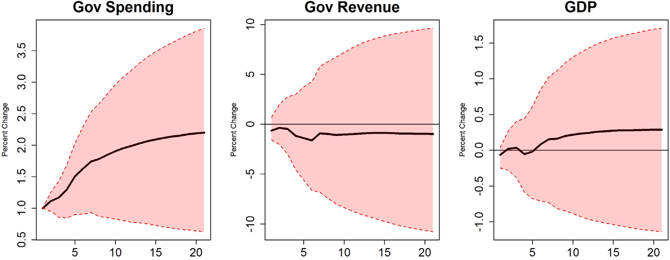
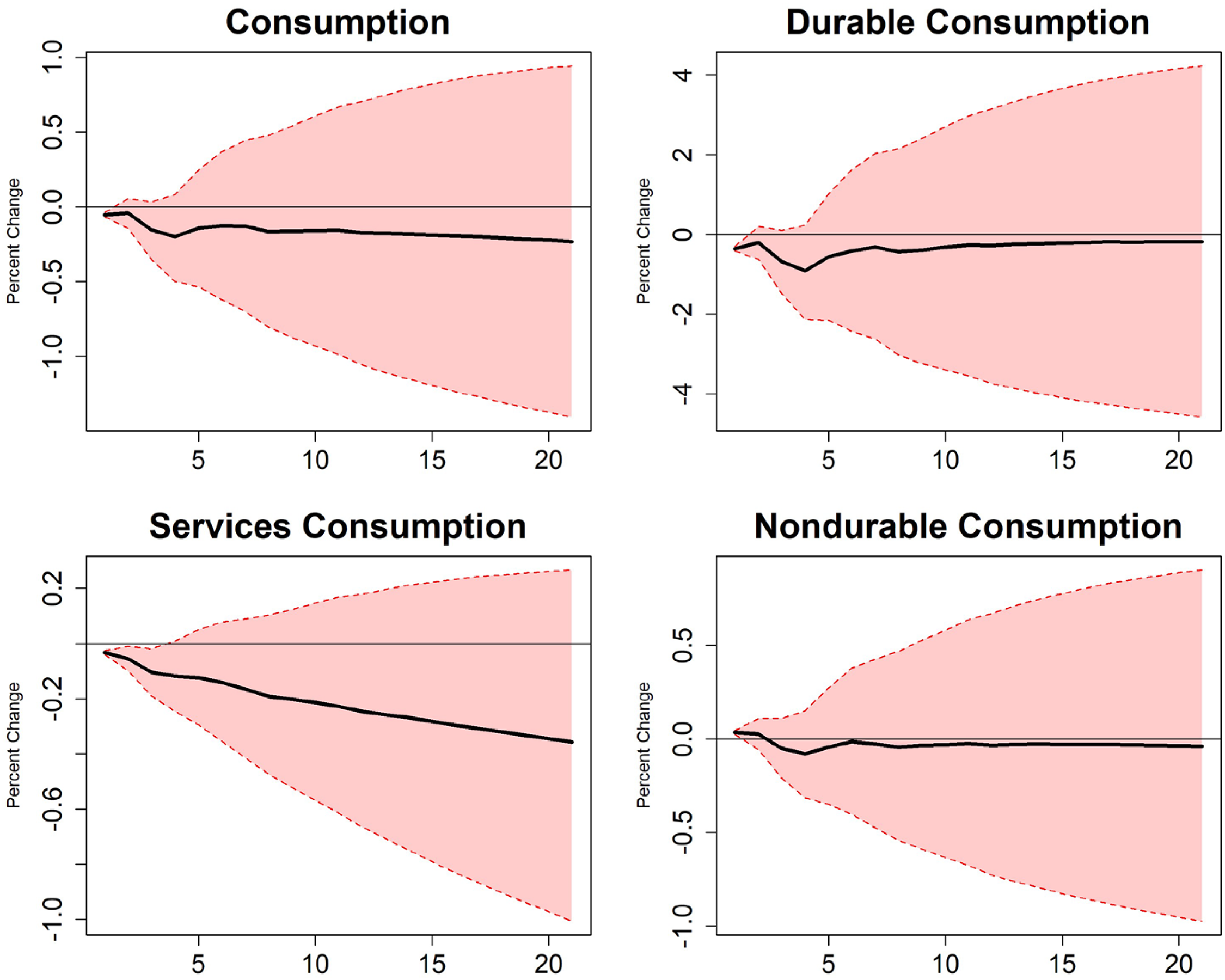
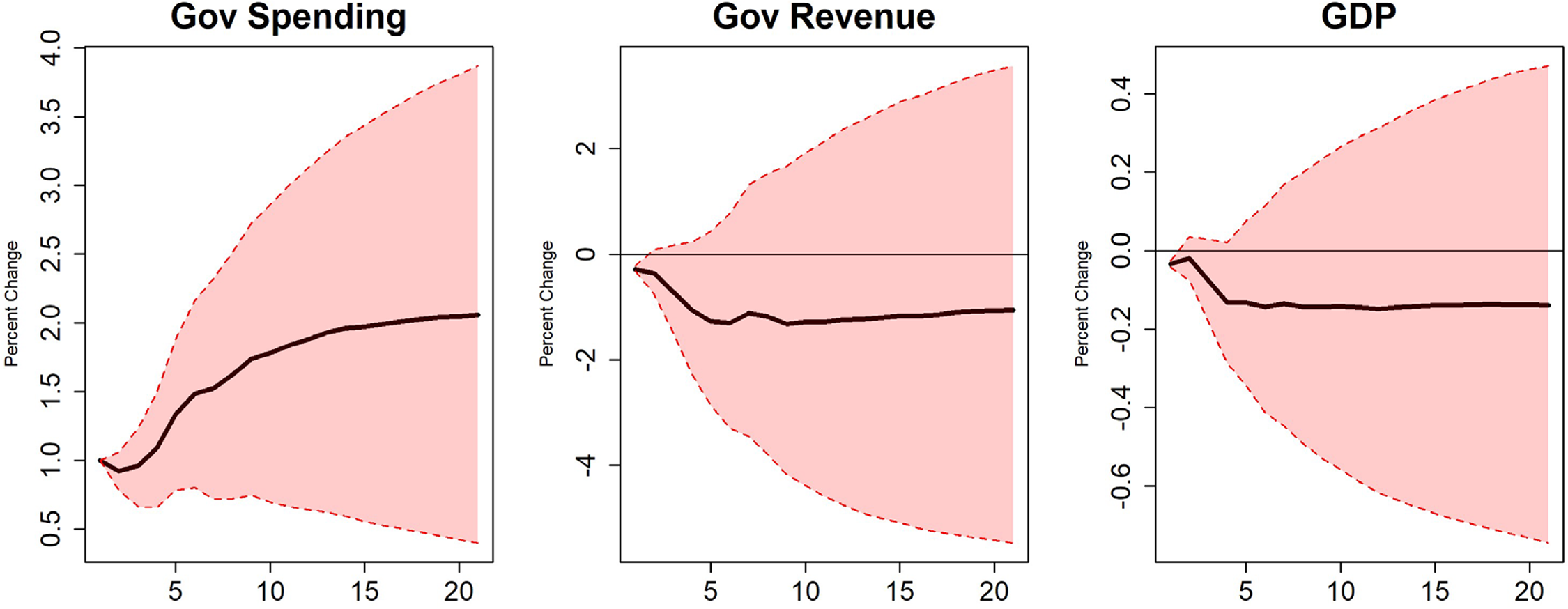
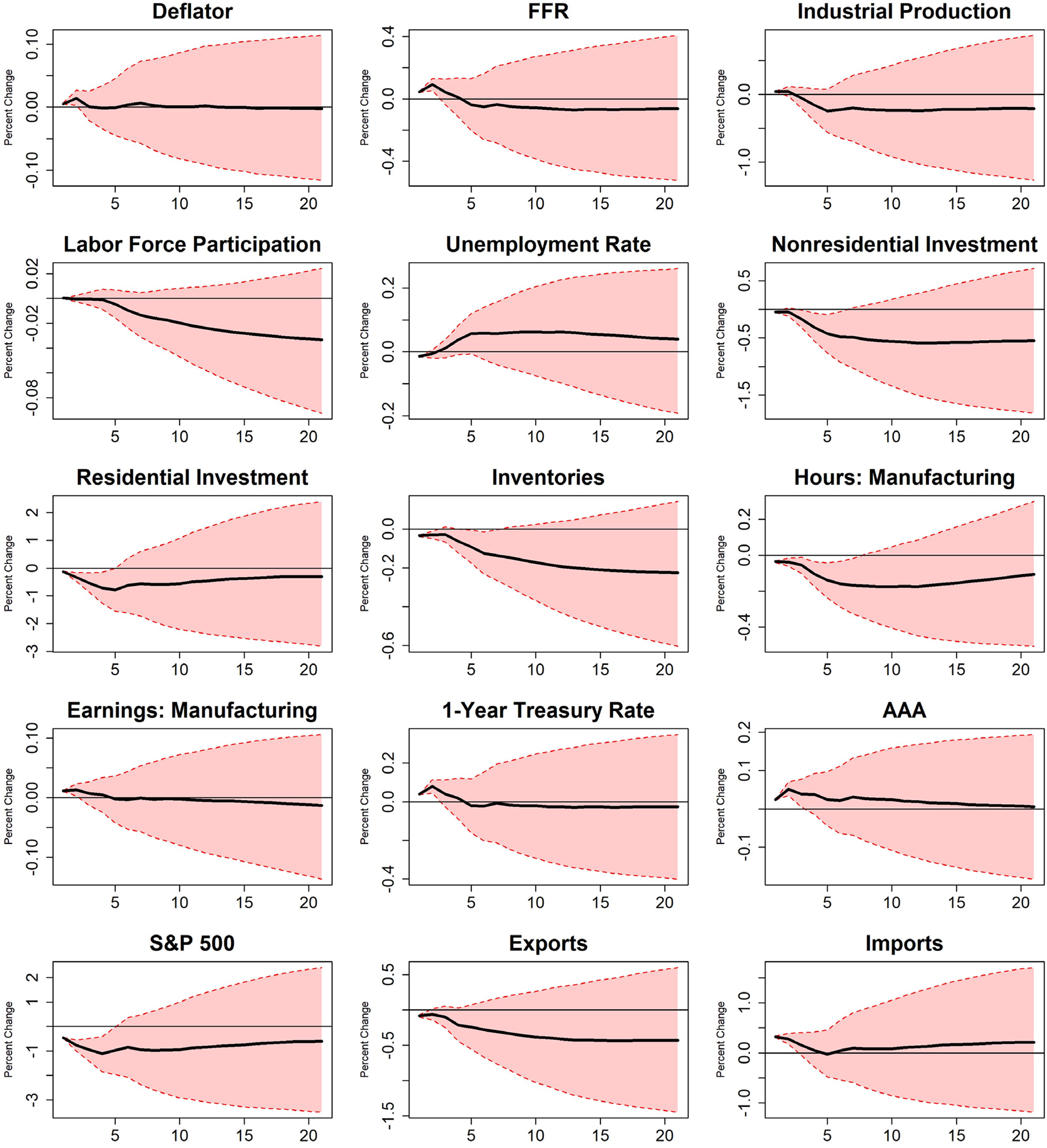
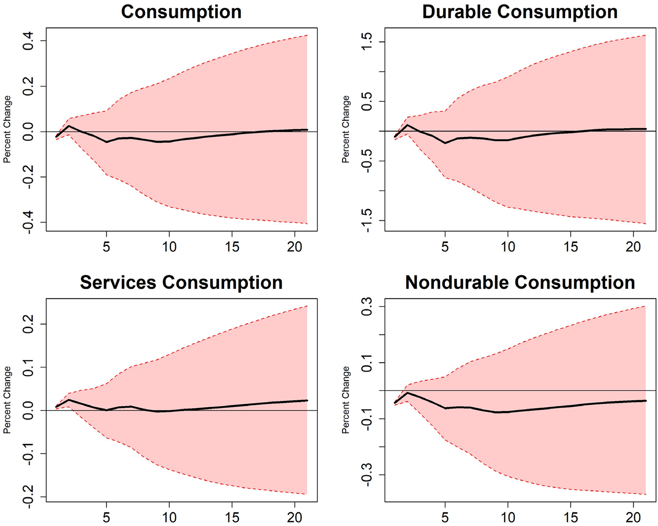
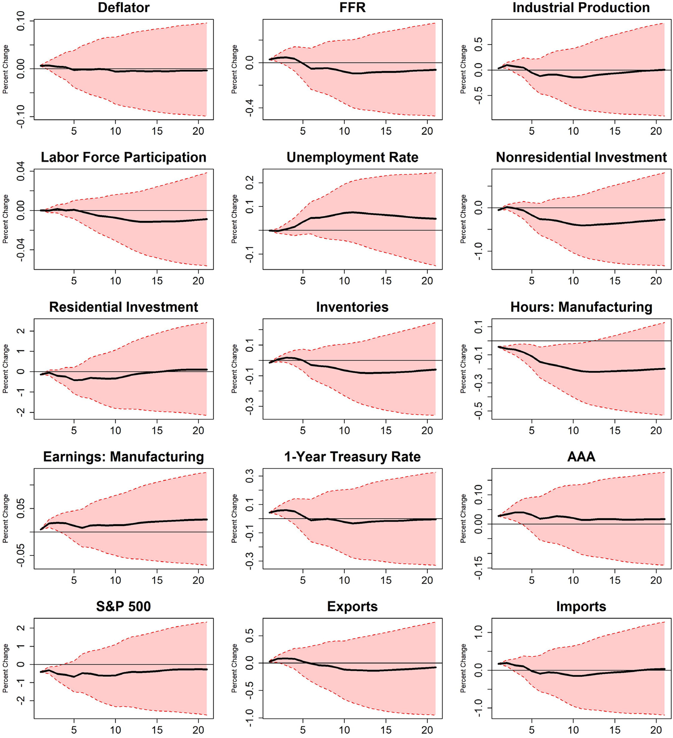
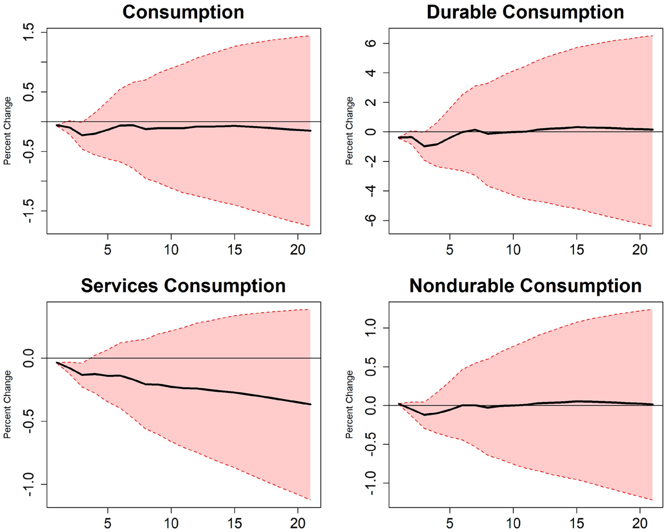
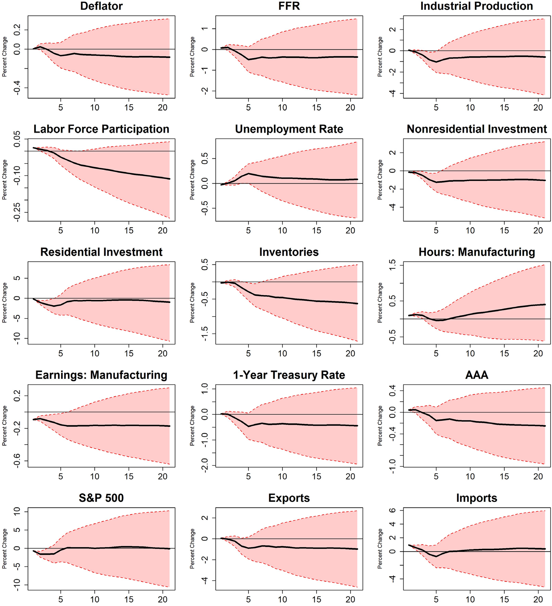
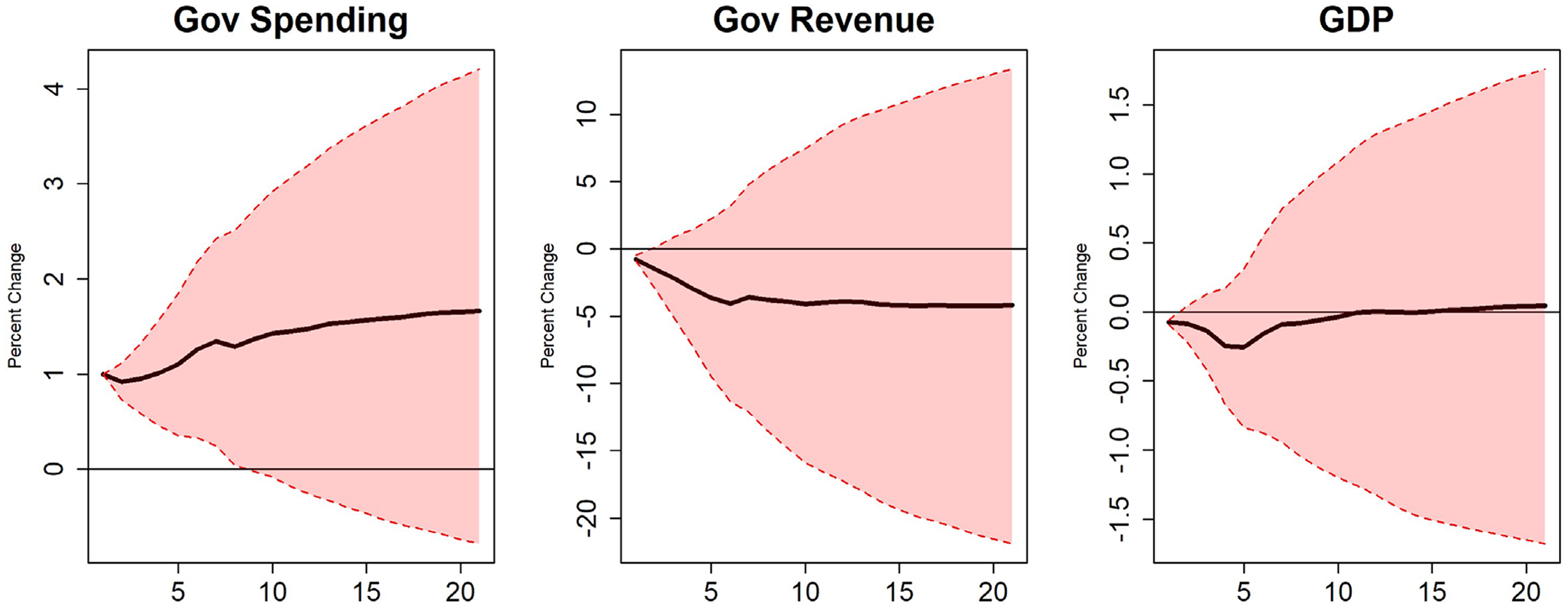
Five Latent Factors

While the efficiency criteria provided by Bai and Ng (2002) suggest the use of three factors, five factors are the minimum number of factors needed for informational sufficiency. The IRFs for the model with five factors are summarized by Figures 5–8.

Figure 5.

Five factors part 1.

Figure 6.

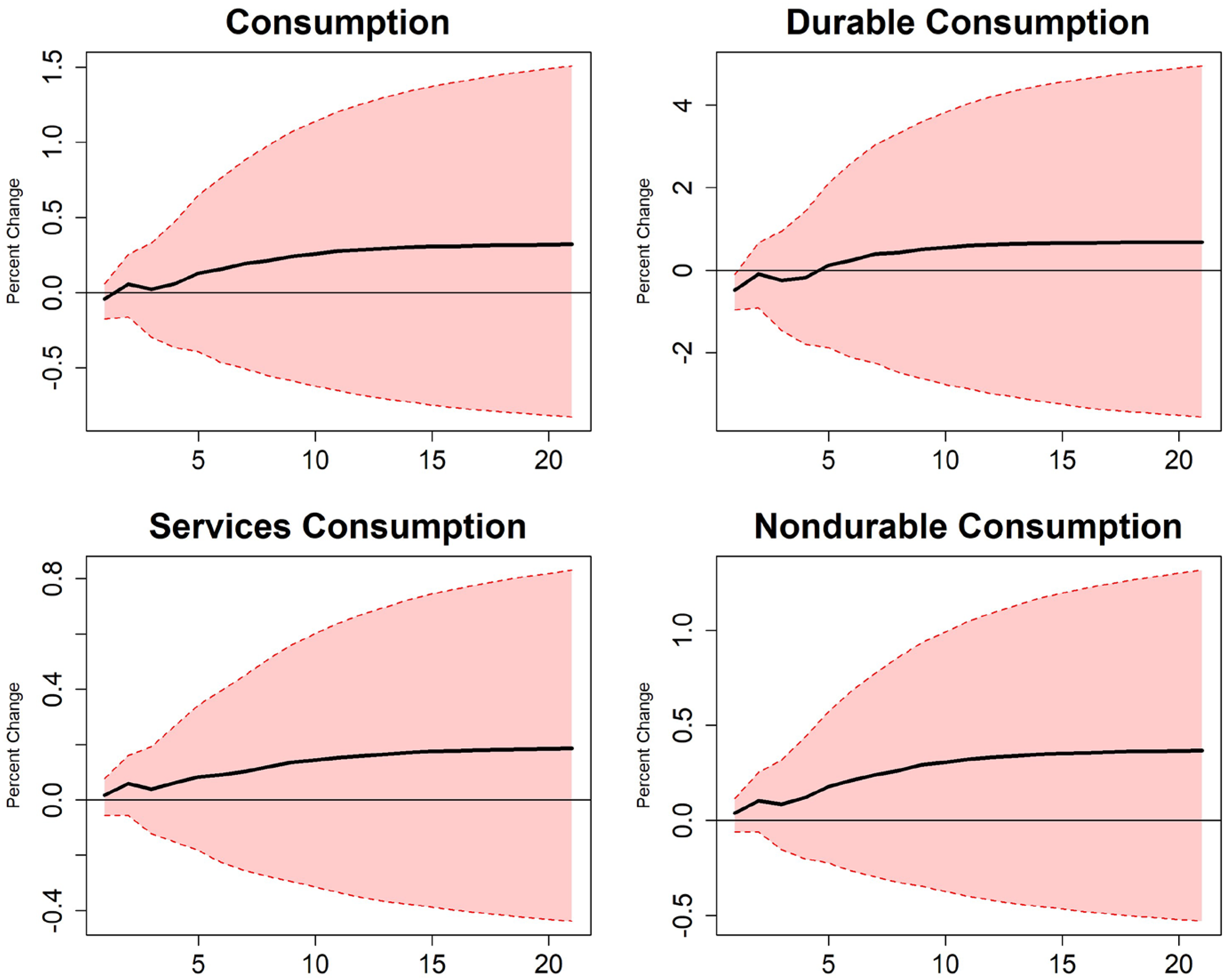
Five factors part 2.

Figure 7.

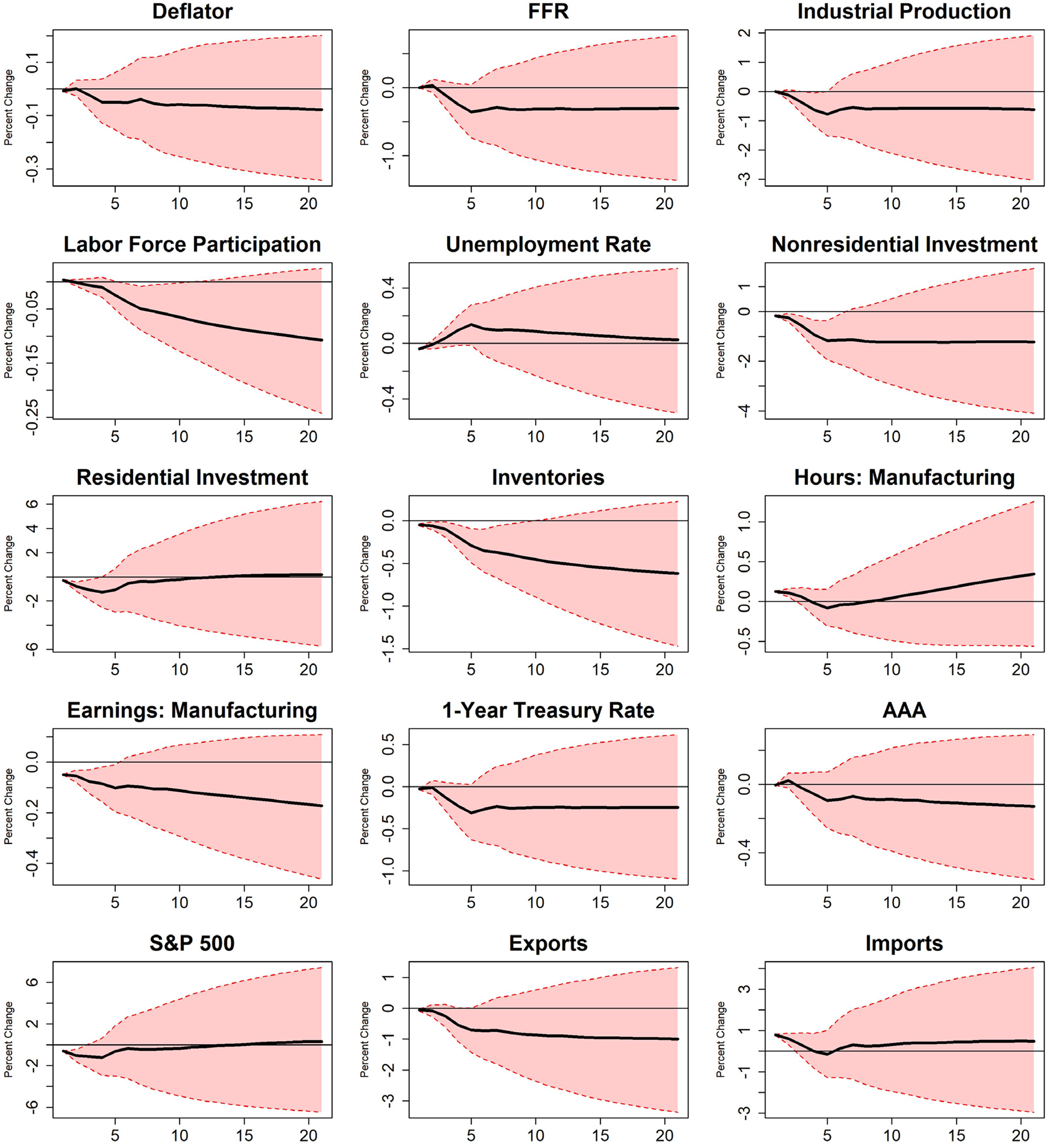
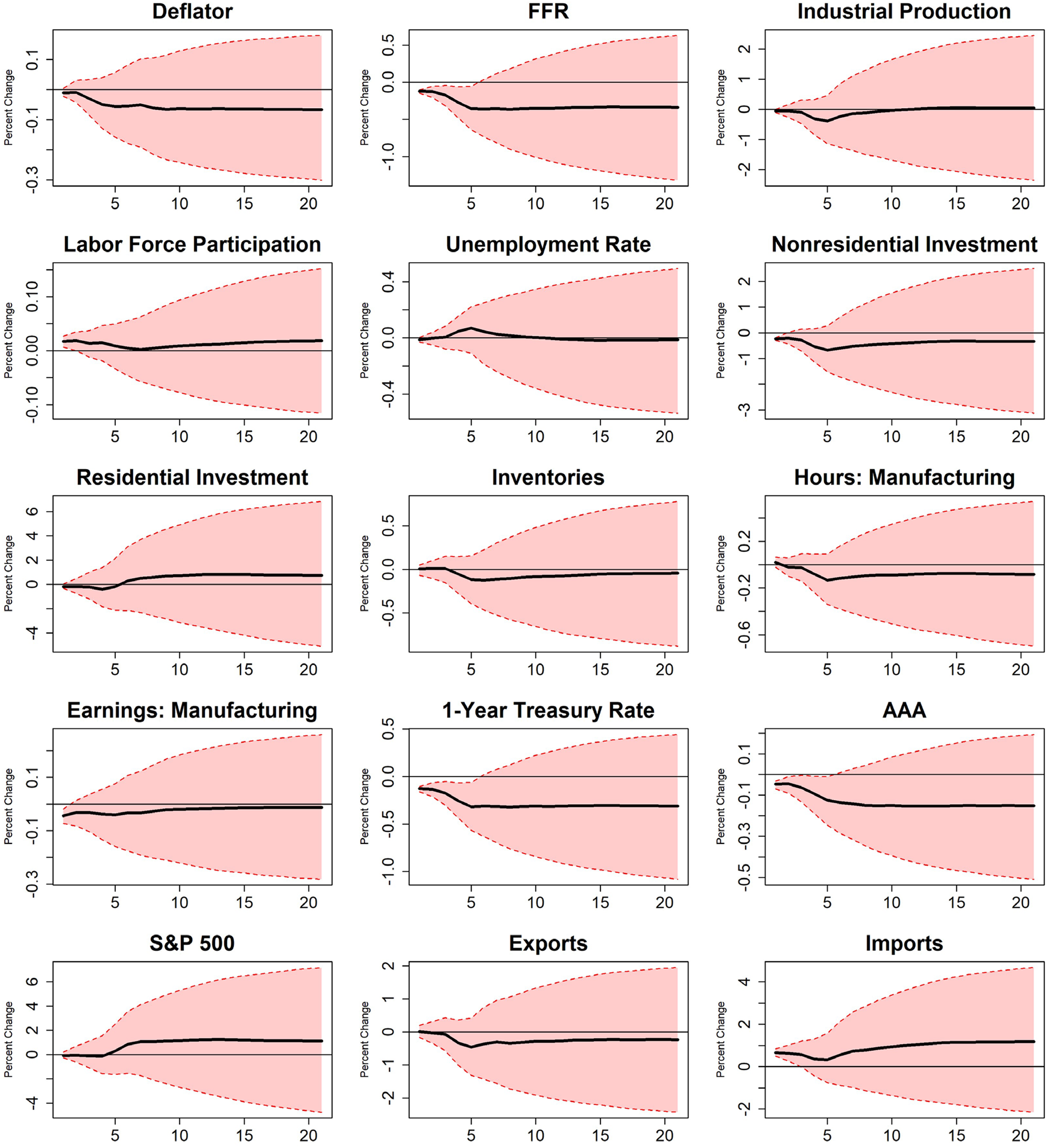
Five factors part 3.

Figure 8.

Defense expenditures part 1.

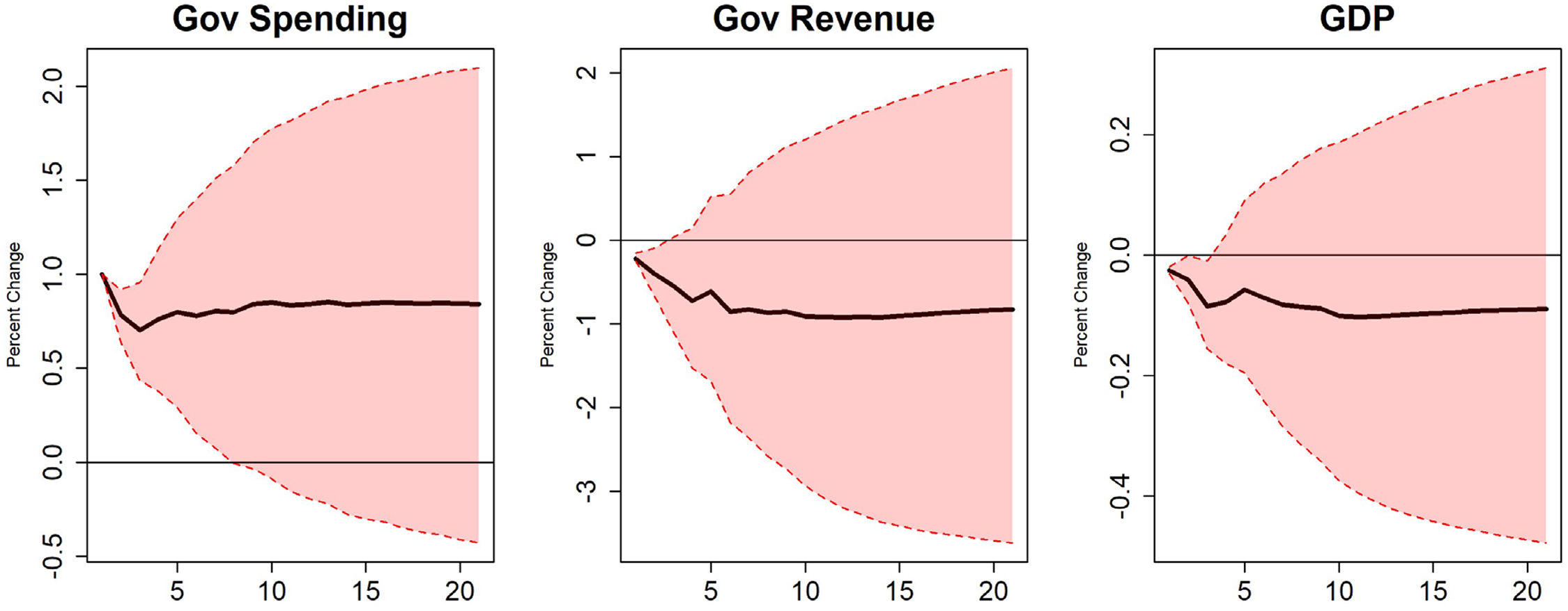
With a greater quantity of information present, there is now a negative effect on output which is statistically significant. The cumulative effect on output is negative for all 20 periods. The peak output multiplier is still positive at 0.358, but all the other multipliers are negative, with the initial multiplier being −0.347. The integral and present-value multipliers are −0.767 and −0.752, respectively. There is also a significantly negative effect on total revenue, which is inconsistent with the findings of Blanchard and Perotti (2002).

A common finding in the literature is that output responses to government spending shocks are often persistent, with effects lasting several quarters. However, this is not a universal result. For example, Blanchard and Perotti's baseline specification, which relies on structural timing (ST) assumptions and focuses on non-defense spending, yields a transitory response similar to the one found in my zero-factor model. This suggests that short-lived effects are not a result of factor augmentation, but instead reflect the identification strategy and the aggregation of spending types. The more persistent responses in BP arise primarily under decision-timing (DT) assumptions or when using defense spending shocks. In contrast, many studies reporting large and persistent output effects rely on signrestricted SVARs. As Fry and Pagan (2011) caution, these models can give a misleading impression of precision. The reported impulse responses reflect variation across admissible sign patterns rather than a uniquely identified structural model, and the resulting bands are often mistaken for statistical confidence intervals. This distinction may explain why my more tightly identified estimates yield more transitory effects than those found in much of the sign-restricted literature.

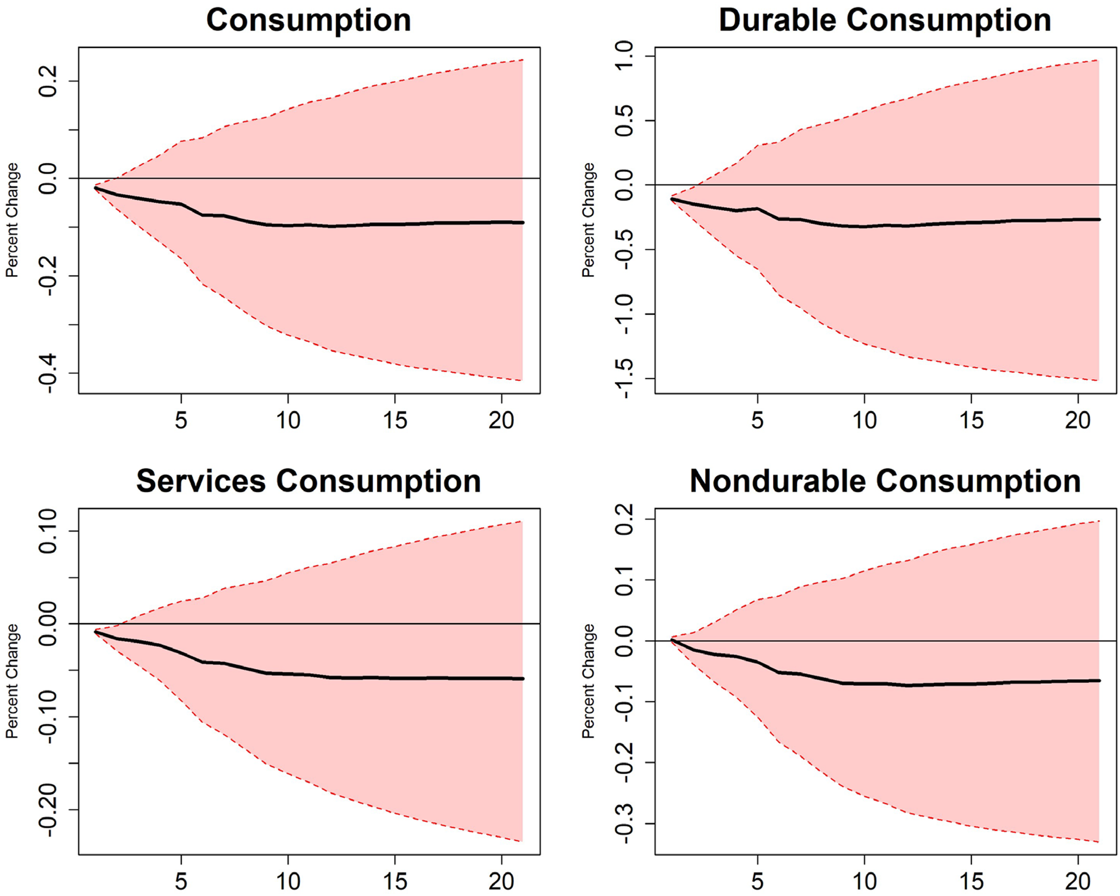
Consumption has an initial multiplier of −0.161 in response to a 1% increase in government spending, with a cumulative multiplier slightly larger than −0.447. A drop in durable consumption and services contributes to the overall decline, with a slight increase in nondurable consumption being the only exception. The five-factor model still shows a decline in nonresidential investment and manufacturing earnings, and a very substantial increase in imports of almost 1%. However, the five-factor model presents somewhat stronger indications of crowding out compared to the three-factor case, though not all effects are statistically significant or persistent. There is now a decline in industrial production, residential investment, and inventories. The unemployment rate initially decreases, but eventually increases relative to where it started. The labor force participation rate declines. Exports fall along with the increase in imports. Financial markets exhibit movements that may be consistent with crowding out, including increases in the federal funds and AAA bond rates and a decline in the S&P 500 index.

Including more factors had a substantial effect on the results of the model with no discernible loss in the precision of the estimates. Therefore, the model with five latent factors is the baseline model to which all subsequent models are compared. The following specifications include five latent factors.

Defense vs. Non-Defense Spending

To address concerns about fiscal foresight (e.g., Ramey 2011a), I examine defense and non-defense spending separately. Defense spending is widely viewed as more plausibly exogenous, while non-defense categories are more likely to be anticipated by economic agents. This distinction allows for comparison of multiplier effects under different assumptions about anticipation.

Figures 8–10 display the impulse responses to a 1% increase in federal defense spending. The initial output multiplier is −0.511, with a peak of 0.225. These values are more negative than the baseline specification and smaller than Ramey's (2011a) narrative-based estimates, which fall between 0.6 and 0.8. Consumption responds negatively, with an initial multiplier of −0.241 and a cumulative value of −0.774, suggesting a more pronounced crowding-out pattern for private demand relative to the aggregate spending model. Financial markets respond sharply: the federal funds rate, 1-year Treasury rate, and AAA bond yields all increase, while the S&P 500 declines. Price effects are moderate but positive, and both forms of investment decline. Imports increase while exports fall, echoing patterns from the total spending specification.

Figure 9.

Defense expenditures part 2.

Figure 10.

Defense expenditures part 3.

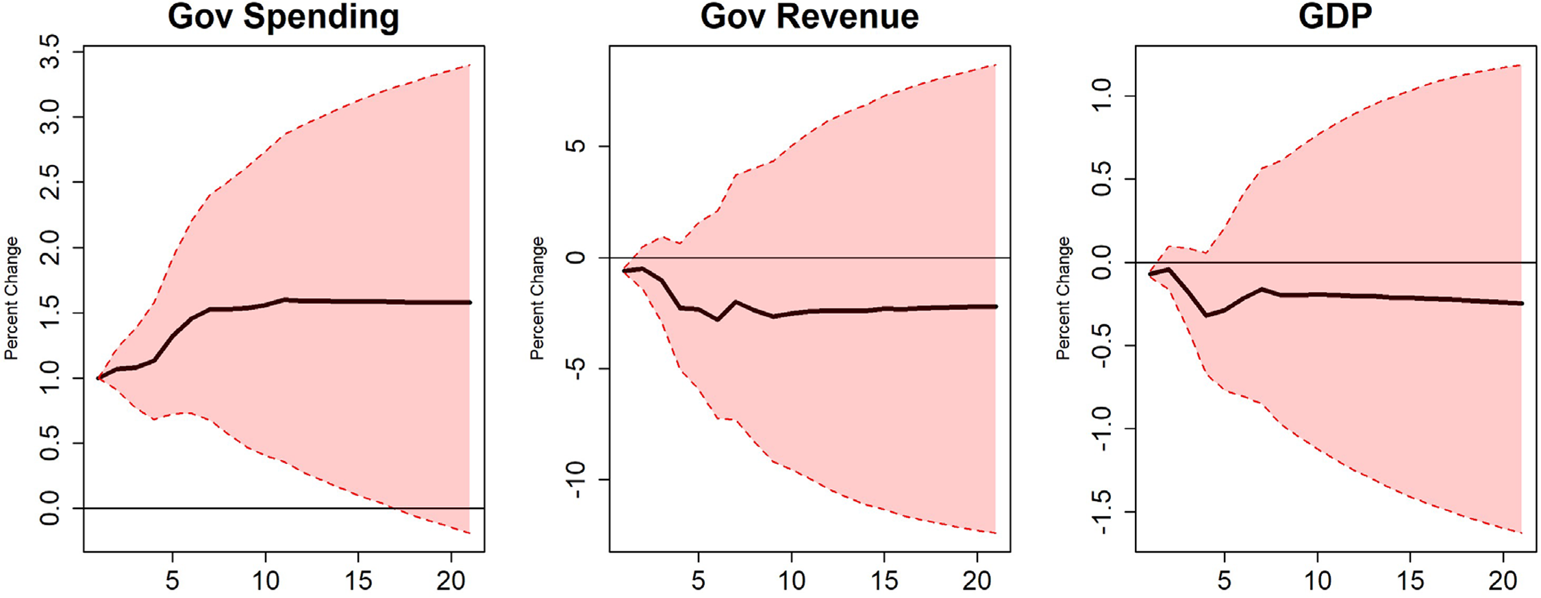
Non-defense spending produces the most severe negative effects in terms of both magnitude and scope across all specifications. Figures 11–13 present these results. The initial output multiplier is −0.893, and although the peak output multiplier rises to 0.698, the initial drop is more severe than in any other case. Consumption falls even more strongly than under defense shocks, with an initial consumption multiplier of −0.435 and a cumulative consumption multiplier of −2.372, driven primarily by a sharp decline in durable goods consumption. Industrial production rises briefly before falling, and some financial indicators suggest more pronounced crowding-out effects: the price deflator and imports rise, while equity markets fall.

Figure 11.

Non-defense expenditures part 1.

Figure 12.

Non-defense expenditures part 2.

Figure 13.

Non-defense expenditures part 3.

Labor market responses under non-defense shocks are mixed. Manufacturing hours and labor force participation rise modestly, but the unemployment rate increases significantly, suggesting dislocation effects that offset any short-term demand stimulus.

Overall, the contrast between defense and non-defense spending reinforces the importance of disaggregating fiscal shocks and accounting for anticipation. Non-defense shocks appear more contractionary, particularly for consumption, and exhibit stronger signs of financial crowding out.

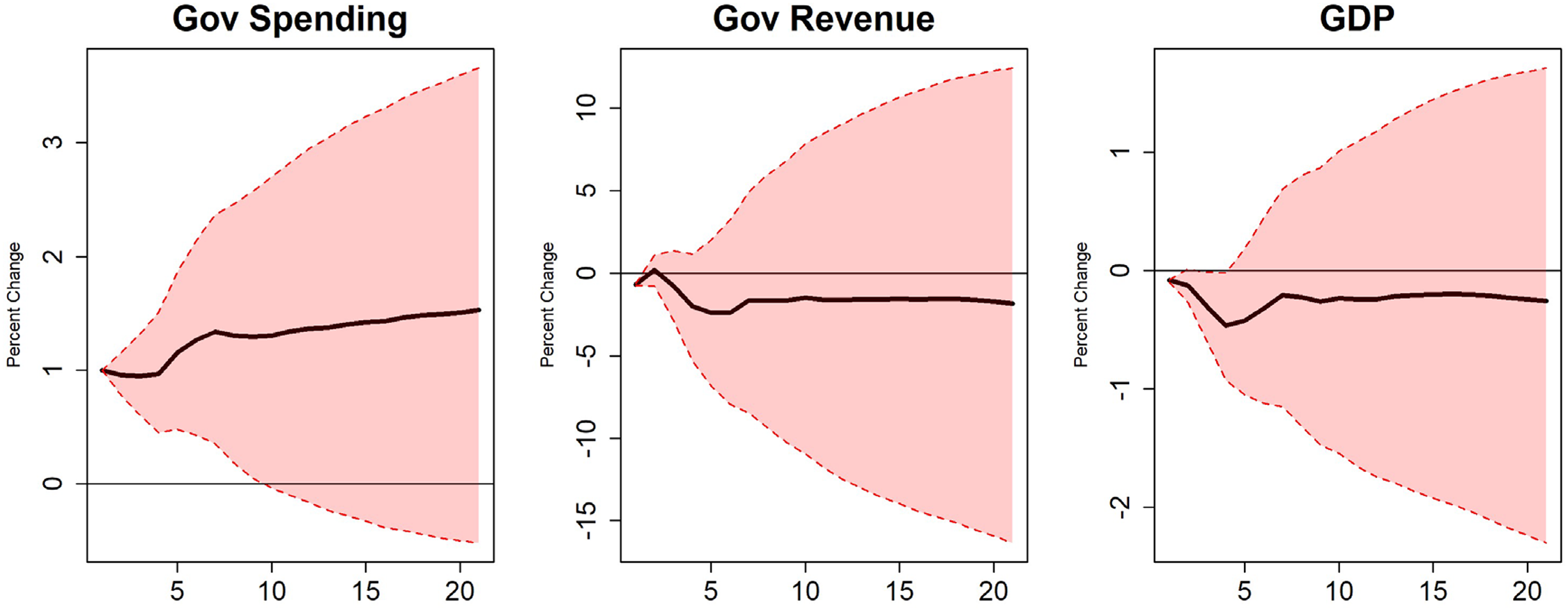
Government Investment

Among all specifications, government investment has the most expansionary output response. Figures 14–16 present these results. While the initial output effect is negative, it is quickly reversed. The peak multiplier reaches 2.131, and the cumulative multiplier is 1.383. Consumption declines initially, driven by reductions in durable and nondurable goods, though services consumption increases. Despite the large output response, investment and equity markets still fall, interest rates rise, and imports increase. These financial and trade responses may reflect continued pressure on private sector activity, though the net effect on output remains positive in this case. Given its notably different pattern of results relative to other government spending categories, I treat government investment as a core specification. Unlike government consumption, which exhibits more modest multipliers and stronger indications of crowding out, investment spending yields persistently strong output effects despite early declines in private activity.

Figure 14.

Government investment expenditures part 1.

Figure 15.

Government investment expenditures part 2.

Figure 16.

Government investment expenditures part 3.

Other Government Spending Categories

In addition to total government spending, defense, non-defense, and investment, I estimate the effects of several other government spending components using the same five-factor specification. These results are summarized in Tables 1 and 2. To conserve space, I report only the multipliers and omit the impulse response figures.

State and Local Expenditures. Replacing federal spending with state and local government expenditures reveals qualitatively similar dynamics. A 1% increase in state and local spending results in a statistically significant decline in output with an initial multiplier of −0.702, a peak multiplier of 1.363, and a cumulative multiplier of 0.287. Consumption is crowded out (initial multiplier: −0.323), and industrial production and both forms of investment decline, along with manufacturing earnings. Interest rates rise, lending additional support to the possibility of financial crowding out, though effects are not uniformly strong across all specifications.

Government Consumption. Government consumption includes goods and services provision such as education and defense. A 1% increase in consumption spending yields an initial output multiplier of −0.430, a peak of 0.871, and a cumulative multiplier of 0.863. Consumption shows a modest initial decline (−0.198 initial multiplier), and the overall pattern remains consistent with other specifications: both forms of investment fall, interest rates rise, and the S&P 500 declines. Notably, industrial production briefly rises, and the price level drops slightly.

Together, these results emphasize that disaggregating fiscal shocks is critical for identifying which forms of government spending are expansionary and which are contractionary. Government consumption, defense, and non-defense spending all display initial contractions and signs of crowding out. By contrast, investment spending stands out as uniquely stimulative in this framework, with both peak and cumulative multipliers exceeding unity.

Robustness

Several papers, including Ramey (2011a, 2011b) and Leeper, Walker and Yang (2010), emphasize the challenge of fiscal foresight. When agents anticipate policy changes, standard VAR estimates may be biased. While the FAVAR framework mitigates this issue by incorporating a broad informational dataset that captures many of the same variables agents use to form expectations, I conduct two additional checks that introduce forecast data more explicitly to test whether unmodeled anticipation alters the results.

The first approach includes a direct forecast of government spending, adapted from Auerbach and Gorodnichenko (2012). The second enriches the factor construction process by including macroeconomic forecasts from the Survey of Professional Forecasters (SPF). If these specifications yield results that differ meaningfully from the baseline, it would suggest that anticipation plays a significant role. If they remain consistent, it supports the interpretation that the FAVAR already internalizes the expectations relevant for identifying unanticipated fiscal shocks.

Government Spending Forecasts (Auerbach and Gorodnichenko)

To explicitly account for anticipated government spending, I include quarterly forecasts adapted from the University of Michigan's Research Seminar in Quantitative Economics (RSQE) macroeconometric model, following the approach of Auerbach and Gorodnichenko (2012). The log-differenced forecast enters the VAR before actual spending but after the factors, preserving causal ordering while isolating surprises. This timing structure allows the model to isolate the unanticipated component of fiscal policy.

Figures 17–19 present the impulse response functions. The estimated effects closely resemble those in the baseline five-factor model. For example, the initial multiplier on output is −0.401 (compared to −0.347 in the baseline), and the peak multiplier is 0.554 (versus 0.358). This similarity suggests that the informational dataset already incorporates most of the forward-looking dynamics captured by the spending forecast, and that fiscal foresight does not meaningfully alter the estimated responses.

Figure 17.

Government forecast part 1.

Figure 18.

Government forecast part 2.

Figure 19.

Government forecast part 3.

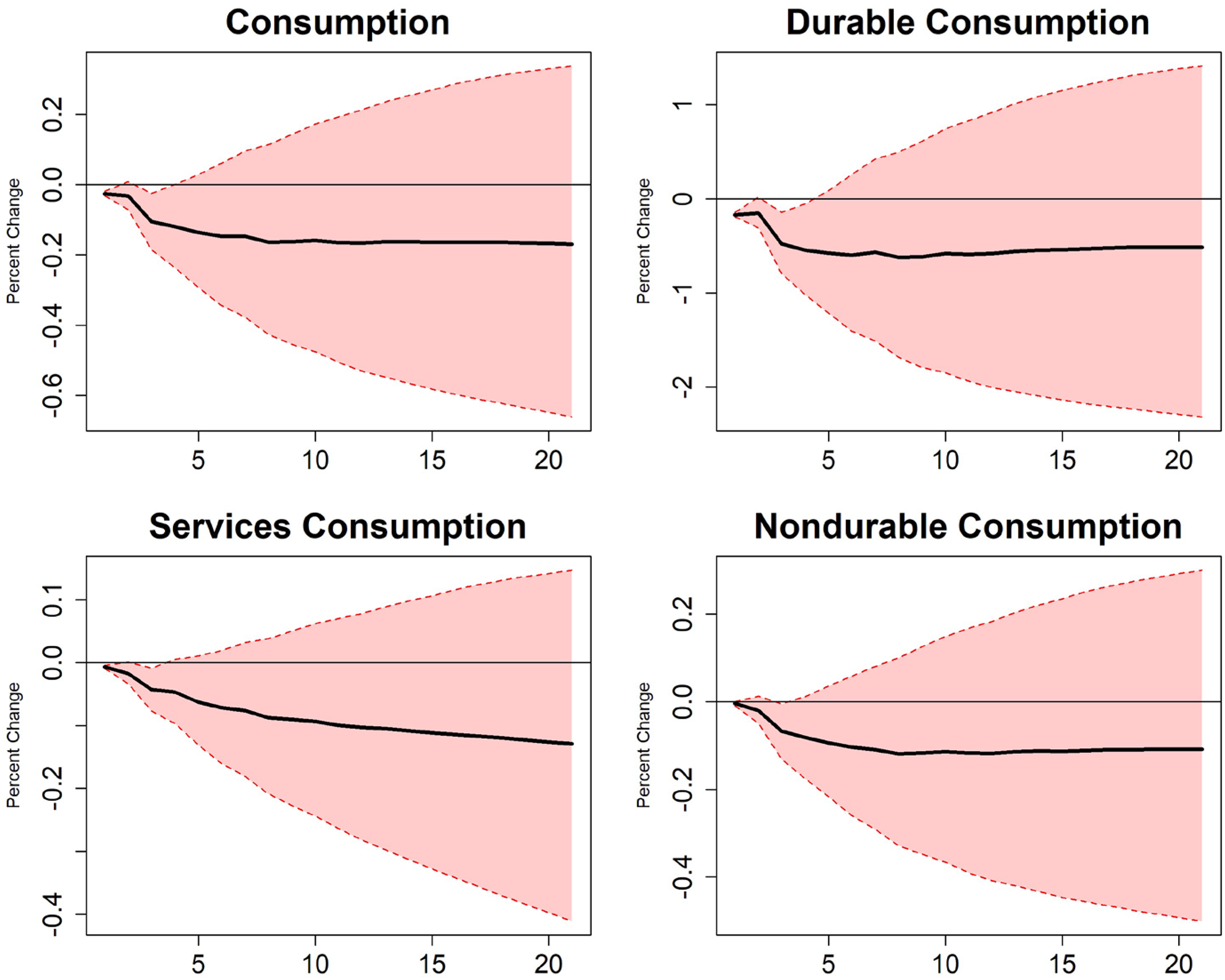
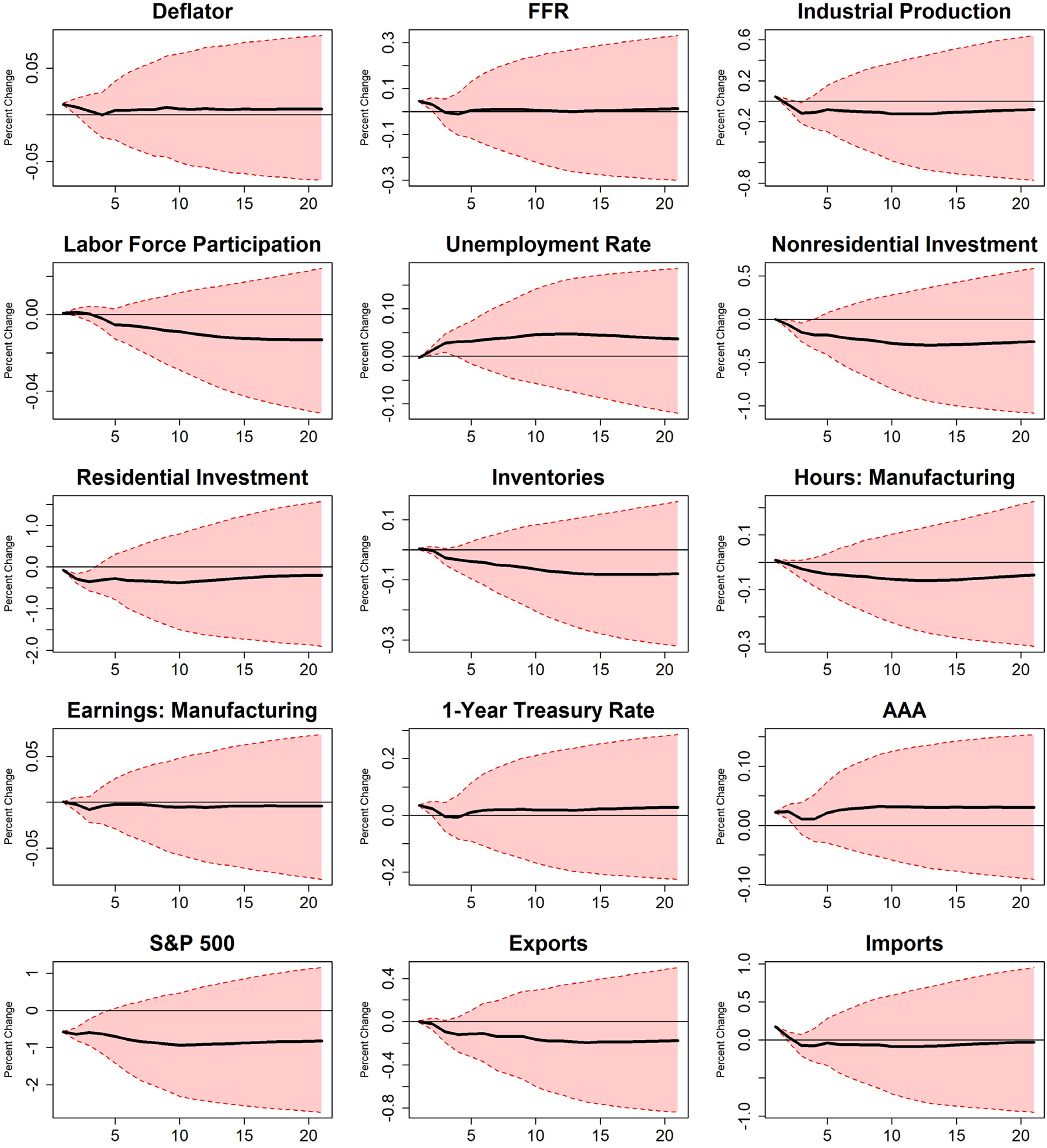
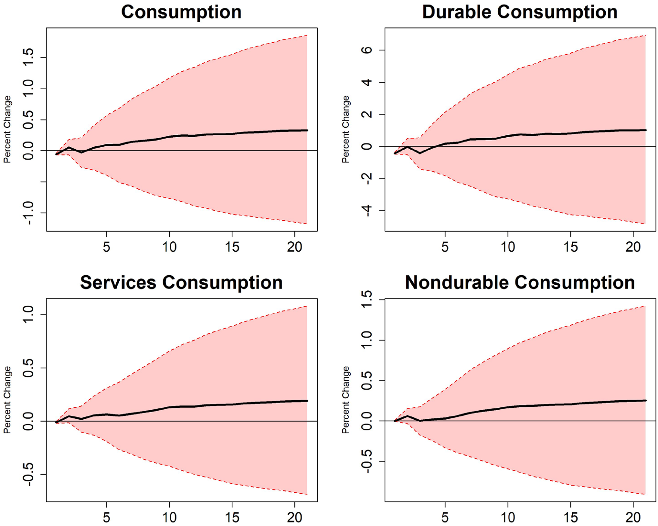
Survey of Professional Forecasters

As a complementary approach, I expand the informational dataset to include expectations from the Survey of Professional Forecasters (SPF). The SPF provides forecasts for output, inflation, consumption, interest rates, and government spending. These data are logdifferenced and added to the informational dataset used to construct the factors. Because the SPF begins in 1981, the sample is restricted to 1981–2019.

Figures 20–22 show results broadly consistent with the baseline, though some modest differences emerge. The cumulative multiplier on output is slightly less negative, and the cumulative consumption multiplier becomes positive. Notably, while the initial consumption response remains negative and statistically significant, later effects are generally not significant. While changes to secondary variables are limited, reversals in manufacturing hours and earnings suggest that some crowding-out effects may be sensitive to expectations.

Figure 20.

Survey of professional forecasters part 1.

Figure 21.

Survey of professional forecasters part 2.

Figure 22.

Survey of professional forecasters part 3.

To ensure these differences are not driven by the restricted time period, I re-estimate the baseline five-factor model using the same 1981–2019 sample. As shown in Tables 1 and 2, the results are very similar to the original baseline. Taken together, these robustness checks suggest that the baseline findings are not driven by unmodeled anticipation effects. The similarity of results across specifications that explicitly incorporate forecast data supports the conclusion that the FAVAR framework sufficiently captures relevant expectations.

The SPF data include forecasts for each variable at one- through five-quarter horizons. All five forecast horizons are included in the informational dataset used to construct the factors. This approach allows the model to reflect a wide range of possible anticipatory behaviors. Incorporating all horizons avoids reliance on any single assumption about agents’ anticipation horizon. The similarity of these results to the baseline therefore supports the robustness of the findings to variations in forecast horizon.

Alternative Identification Ordering

To further test the robustness of the results, I consider an alternative identification strategy in which government spending is ordered after taxes. This adjustment evaluates the sensitivity of the impulse responses to plausible changes in the assumed shock structure, as fiscal policy components are often jointly determined.

The estimated multipliers remain closely aligned with the baseline model. As reported in Tables 1 and 2, the peak output multiplier is 0.432 (compared to 0.358 in the baseline), and the cumulative present value multiplier is −0.576 (vs. −0.752). Similarly, the consumption response remains negative and statistically significant on impact, with a slightly smaller magnitude. These results suggest that the main conclusions are not sensitive to this identification choice, reinforcing the credibility of the baseline findings.

Lag Length and Factor Count

I also examine whether the main results are sensitive to the number of lags in the VAR or the number of factors included in the model. The baseline specification uses five lags and five factors. Five lags is a standard choice for quarterly macroeconomic data. The number of factors is chosen based on the informational sufficiency test.

To assess robustness, I first re-estimate the baseline model using seven lags instead of five. The impulse response functions are nearly identical, and the multipliers reported in Table 1 show no changes. This confirms that the short-lived nature of the responses is not an artifact of the lag structure.

Next, I re-estimate the model with seven factors instead of five. The resulting GDP multipliers are somewhat more negative, but the overall conclusions remain unchanged. This suggests that the baseline specification includes a sufficient number of factors and that the findings are not sensitive to moderate increases in factor dimensionality.

Together, these checks confirm that the main results are robust to reasonable variations in lag length and factor count. The finding that spending shocks have limited or negative effects on output holds across these alternative specifications.

Conclusion

This paper revisits the fiscal multiplier debate by applying a factor-augmented VAR framework to a broad dataset covering U.S. macroeconomic conditions from 1960 to 2019. I find that augmenting a traditional VAR with principal components derived from over 200 macroeconomic series substantially alters the estimated effects of government spending shocks. Specifically, whereas a baseline VAR closely replicates the expansionary short-run responses found in Blanchard and Perotti (2002), incorporating latent factors often weakens or even reverses these effects. In all five-factor specifications, the initial responses of output and consumption are negative, with little evidence of sustained long-run gains.

These patterns hold across multiple disaggregated spending categories and persist in robustness checks that explicitly incorporate forward-looking data to address concerns regarding fiscal foresight. Only government investment consistently yields a delayed expansionary response following an initial contraction. This suggests that the composition of spending significantly influences macroeconomic effects. Furthermore, the results indicate that government spending tends to crowd out private investment and net exports, particularly in the short run.

Methodologically, the paper demonstrates how expanding the information set in structural VARs can meaningfully shift our understanding of fiscal transmission. The FAVAR approach provides a more comprehensive view of the economic environment and implicitly accounts for anticipatory behavior that may otherwise bias conventional estimates. The robustness of results to the inclusion of explicit forecasts further supports this interpretation. In addition, I contrast these findings with studies using sign-restricted SVARs, which may understate uncertainty and impose assumptions that exclude contractionary responses by construction.

Taken together, the evidence calls into question the generality of the expansionary multipliers often reported in small-scale or sign-restricted VAR studies. It also highlights how model design, especially identification strategy, variable selection, and dimensionality, can shape empirical conclusions. While this paper deliberately excludes the COVID-19 period due to its exceptional nature, future research could use pandemic-era data to assess whether the contractionary responses documented here extend to extreme fiscal interventions, potentially using nonlinear or regime-switching models.

More broadly, the findings suggest that the effectiveness of fiscal policy is both statedependent and composition-sensitive, with important implications for stabilization efforts. In particular, the evidence challenges the notion that government spending is reliably expansionary and instead highlights the risk of short-run crowding out across key sectors. Disentangling these dynamics remains a vital area for further empirical and theoretical work. Future research should investigate whether the contractionary responses identified here generalize to other institutional settings, including emerging economies, and whether they persist in the context of extreme interventions such as those undertaken during the COVID-19 pandemic.

Supplemental Material

sj-docx-1-pfr-10.1177_10911421251391425 - Supplemental material for Measuring the Effect of Government Spending Shocks on Output: A Factor-Augmented VAR Approach

Supplemental material, sj-docx-1-pfr-10.1177_10911421251391425 for Measuring the Effect of Government Spending Shocks on Output: A Factor-Augmented VAR Approach by Philip Vinson in Public Finance Review

Footnotes

Declaration of Conflicting Interests

The author declared no potential conflicts of interest with respect to the research, authorship, and/or publication of this article.

Funding

The author received no financial support for the research, authorship, and/or publication of this article.

ORCID iD

Philip Vinson

Supplemental material

Supplemental material for this article is available online.

Author Biography

Philip Vinson is an Associate Professor in Economics. His area of research is in macroeconomics with a focus on fiscal policy, housing, and education.

References

Auerbach

A. J.

Gorodnichenko

. 2012. “Measuring the Output Responses to Fiscal Policy.” American Economic Journal: Economic Policy 4 (2): 1–27. https://doi.org/10.1257/pol.4.2.1

Bai

. 2002. “Determining the Number of Factors in Approximate Factor Models.” Econometrica 70 (1): 191–221. https://doi.org/10.1111/1468-0262.00273

Baumeister

Hamilton

J. D.

. 2015. “Sign Restrictions, Structural Vector Autoregressions, and Useful Prior Information.” Econometrica 83 (5): 1963–1999. https://doi.org/10.3982/ECTA12356

Bernanke

B. S.

Boivin

Eliasz

. 2005. “Measuring the Effects of Monetary Policy: A Factor-Augmented Vector Autoregressive (FAVAR) Approach.” The Quarterly Journal of Economics 120 (1): 387–422. https://doi.org/10.1162/0033553053327452

Blanchard

Perotti

. 2002. “An Empirical Characterization of the Dynamic Effects of Changes in Government Spending and Taxes on Output.” The Quarterly Journal of Economics 117 (4): 1329–1368. https://doi.org/10.1162/003355302320935043

Deb

Furceri

Ostry

J. D.

Tawk

Yang

. 2024. “The Effects of Fiscal Measures during COVID-19.” Journal of Money, Credit and Banking: 1597–1621. https://doi.org/10.1111/jmcb.13154

Faria-e-Castro

2021. “Fiscal Policy During a Pandemic.” Journal of Economic Dynamics and Control 125: 104088. https://doi.org/10.1016/j.jedc.2021.104088 .

Fatas

Mihov

. 2003. “The Case for Restricting Fiscal Policy Discretion.” The Quarterly Journal of Economics 118 (4): 1419–1447. https://doi.org/10.1162/003355303322552838

Forni

Gambetti

. 2010. “Fiscal foresight and the effects of government spending.” Center for Economic Research (RECent) Working Paper No. 049.

10.

Forni

Gambetti

. 2014. “Sufficient Information in Structural VARs.” Journal of Monetary Economics 66: 124–136. https://doi.org/10.1016/j.jmoneco.2014.04.005

11.

Fragetta

Gasteiger

. 2014. “Fiscal Foresight, Limited Information and the Effects of Government Spending Shocks.” Oxford Bulletin of Economics and Statistics 76 (5): 667–692. https://doi.org/10.1111/obes.12036

12.

Fry

Pagan

. 2011. “Sign Restrictions in Structural Vector Autoregressions: A Critical Review.” Journal of Economic Literature 49 (4): 938–960. http://doi.org/10.1257/jel.49.4.938

13.

Gali

Lopez-Salido

J. D.

Vallés

. 2007. “Understanding the Effects of´ Government Spending on Consumption.” Journal of the European Economic Association 5 (1): 227–270. https://doi.org/10.1162/JEEA.2007.5.1.227

14.

Gupta

Kabundi

Ziramba

. 2010. “The Effect of Defense Spending on US Output: A Factor Augmented Vector Autoregression (Favar) Approach.” Defence and Peace Economics 21 (2): 135–147. https://doi.org/10.1080/10242690903569056

15.

Kim

2019. “The Effects of Government Spending in Korea: A FAVAR Approach (in Korean).” Economic Analysis (Quarterly) 25 (3): 100–137. https://www.bok.or.kr/eng/bbs/E0002726/view.do?nttId=10054110&menuNo=400218&pageIndex=1

16.

Laumer

2020. “Government Spending and Heterogeneous Consumption Dynamics.” Journal of Economic Dynamics and Control 114: 103868. https://doi.org/10.1016/j.jedc.2020.103868

17.

Leeper

E. M.

Walker

T. B.

Yang

S. C. S.

. 2010. “Government Investment and Fiscal Stimulus.” Journal of Monetary Economics 57 (8): 1000–1012. https://doi.org/10.1016/j.jmoneco.2010.09.002

18.

Marattin

Salotti

. 2011. “On the Usefulness of Government Spending in the EU Area.” The Journal of Socio-Economics 40 (6): 780–795. https://doi.org/10.1016/j.socec.2011.08.018

19.

McCracken

. 2020. “FRED-QD: A quarterly database for macroeconomic research (NBER Working Paper No. w26872).” National Bureau of Economic Research.

20.

Mountford

Uhlig

. 2009. “What are the Effects of Fiscal Policy Shocks?.” Journal of Applied Econometrics 24 (6): 960–992. https://doi.org/10.1002/jae.1079

21.

Ramey

V. A.

2011a. “Identifying Government Spending Shocks: It’s all in the Timing.” The Quarterly Journal of Economics 126 (1): 1–50. https://doi.org/10.1093/qje/qjq008

22.

Ramey

V. A.

2011b. “Can Government Purchases Stimulate the Economy?.” Journal of Economic Literature 49 (3): 673–685. https://doi.org/10.1257/jel.49.3.673

23.

Ramey

V. A.

Shapiro

M. D.

. 1998. “Costly Capital Reallocation and the Effects of Government Spending.” In Carnegie-Rochester Conference Series on Public Policy, 145–194. Amsterdam, Netherlands: North-Holland.

24.

Stock

J. H.

Watson

M. W.

. 2002. “Forecasting Using Principal Components from a Large Number of Predictors.” Journal of the American Statistical Association 97 (460): 1167–1179. https://doi.org/10.1198/016214502388618960

25.

Tenhofen

Wolff

G. B.

. 2007. Does anticipation of government spending matter? Evidence from an expectation augmented VAR. Bundesbank Series 1 Discussion Paper No. 2007, 14, Available at SSRN: https://ssrn.com/abstract=2785288

26.

van Gemert

Lieb

Treibich

. 2022. “Local Fiscal Multipliers of Different Government Spending Categories.” Empirical Economics 63 (5): 2551–2575. https://doi.org/10.1007/s00181-022-02217-5

Supplementary Material

Please find the following supplemental material available below.

For Open Access articles published under a Creative Commons License, all supplemental material carries the same license as the article it is associated with.

For non-Open Access articles published, all supplemental material carries a non-exclusive license, and permission requests for re-use of supplemental material or any part of supplemental material shall be sent directly to the copyright owner as specified in the copyright notice associated with the article.

0.00 MB

0.05 MB