Sage Journals: Discover world-class research

Abstract

High-content analysis has revolutionized cancer drug discovery by identifying substances that alter the phenotype of a cell, which prevents tumor growth and metastasis. The high-resolution biofluorescence images from assays allow precise quantitative measures enabling the distinction of small molecules of a host cell from a tumor. In this work, we are particularly interested in the application of deep neural networks (DNNs), a cutting-edge machine learning method, to the classification of compounds in chemical mechanisms of action (MOAs). Compound classification has been performed using image-based profiling methods sometimes combined with feature reduction methods such as principal component analysis or factor analysis. In this article, we map the input features of each cell to a particular MOA class without using any treatment-level profiles or feature reduction methods. To the best of our knowledge, this is the first application of DNN in this domain, leveraging single-cell information. Furthermore, we use deep transfer learning (DTL) to alleviate the intensive and computational demanding effort of searching the huge parameter’s space of a DNN. Results show that using this approach, we obtain a 30% speedup and a 2% accuracy improvement.

Keywords

high-content screening image analysis deep transfer learning cancer drug discovery

Introduction

Recent advances in quantitative microscopy and high-performance computing have enabled rapid progress in the development of high-throughput image-based assays. These high-content analysis (HCA) assays allow not only a precise quantitative observation of multiple parameters such as nuclear size, nuclear morphology, DNA replication, and many more subtle features derived from each image, but also the screening of thousands of cells. To tackle this high-throughput high-dimensional problem, biologists tend to use population averages of per-cell information prior to machine learning (ML) algorithms such as principal component analysis, random forest, K-nearest neighbors, or support vector machines. Moreover, a recent survey¹ shows that about 70% of the papers on HCA experiments published in Science, Nature, Cell, and the Proceedings of the National Academy of Sciences from 2000 to 2012 used only one or two of the cell’s measured features, and less than 15% used more than six. Unfortunately, and due to the exponential increase in the number of product terms,² such ML algorithms become impractical for these problems with thousands of samples and hundreds of measured features. As a result, about 85% of the research work in HCA underutilized potentially valuable information that might have helped in speeding up early-stage drug discovery. In this paper, we are interested in exploring state-of-the-art algorithms developed in the field of artificial intelligence to address these high-throughput high-dimensional data.

The discovery of hierarchical visual sensory processing systems in the neocortex of the mammal brain motivated the field of artificial intelligence to develop algorithms to hierarchically extract information from data.^3,4 Deep learning^5,6 has thus emerged as a new paradigm in artificial intelligence focusing on computational models for information representation that exhibit characteristics similar to those of the neocortex, in an attempt to imitate a primate visual system with its sequence of processing stages: detection of edges, primitive shapes, and moving up gradually to more complex visual shapes.^7,8 Since 2006, deep learning research has been successful not only in academia but also in companies such as Google (image retrieval) and Facebook (face recognition). With many application domains, including image recognition^9,10 and speech recognition,¹¹ deep learning has beaten other ML techniques at predicting the activity of potential drug molecules using quantitative structures¹² and predicting the effects of mutations in noncoding DNA on gene expression and disease.¹³

We focus on the challenge of using information content as high as possible, by considering per-cell information and all the available features, to build a classifier for the chemical mechanism of action (MOA). A mechanism of action usually refers to biochemical interaction through which the drug binds to form pharmacological effects. In here, MOA is specifically used to express a share of similar phenotypic outcomes among different compound treatments and not a strict modulation of a particular target or target class.¹⁴ According to Ljosa et al.,¹⁴ the mechanistic classes were selected to provide the data with a wide cross section of cellular morphological phenotypes. We propose a deep transfer learning (DTL) framework, combining the advantages of deep learning with the flexibility of transfer learning. Transfer learning consists of reusing the knowledge gained from a (source) problem to solve a new (target) problem. Ideally, DTL should improve the performance of the reused classifier in the target problem over the baseline, that is, over the classifier trained directly in the target problem.

Our contribution can thus be summarized as follows:

Use of per-cell information with all the extracted features from high-content images

Use of state-of-the-art deep learning models coupled with GPU computational power to analyze such high-throughput high-dimensional data

Use of transfer learning to improve the performance of the models (in terms of computational speed)

In this paper, we consider stacked autoassociators^15,16 (SAAs) as classifiers of MOAs on freely available MFC7 wild-type breast cancer data¹⁴ using a DTL framework that includes a supervised layer-based feature transference approach.^16,17

A possible use case of the work presented in this paper would be for a researcher to (1) solve a given classification problem of MOA or obtain the classifiers used to solve such a problem from the result of a previous work, (2) select what part of a previously developed classifier to transfer, and (3) solve the new problem by doing transfer learning of the learned classifiers for a new MOA task and benefit from a faster training (when compared to a random initialization) and an eventual improvement in classification accuracy. In the case of using deep neural networks as classifiers, as we do in this work, the researcher can choose which layers should be reused from a previous experiment. In the Results section, we discuss several settings and advise the use of the setting that produces the best results in our work.

Materials and Methods

Data

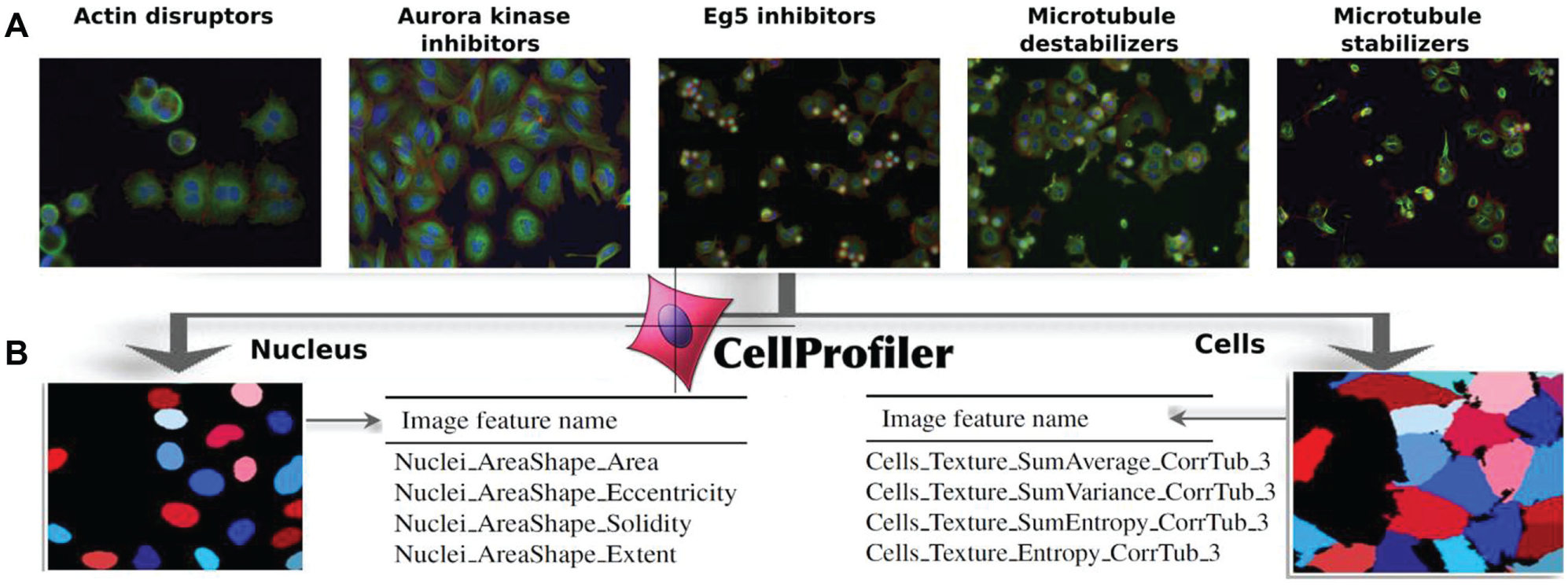
We used a publicly available (http://www.broadinstitute.org/bbbc, accession BBBC021) dataset from the genetically engineered MCF7-wt (breast cancer expressing wild-type p53) cell line.²⁶ Briefly (all details of sample preparation and image analysis can be found in Ljosa et al.¹⁴), images of cell cultures with a given treatment (specific compound × concentration combination) were acquired on a high-content imaging platform using a 16-bit camera. Each image was further segmented using CellProfiler¹⁸ (CP) by identifying nuclear and cytoplasmic boundaries. Then, 453 distinct features for each cell representing a variety of geometric, intensity, subcellular localization, and texture features¹⁹ were extracted with CP. Figure 1 shows some examples of captured images representing some of the MOAs, as well as some of the features extracted with CP.

Figure 1.

(A) Examples of different phenotypes (MOAs) captured after compound incubation of MFC7-wt cells. According to Ljosa et al.,¹⁴ only 6 of the 12 MOAs were visually identifiable. (B) Cell segmentation and feature extraction are performed using CellProfiler.¹⁸ For each cell, a variety of geometric, intensity, subcellular localization, and texture features were extracted.

Our problem consists of predicting the MOA of a given treatment using per-cell information, in contrast to other established methodologies that use some profiling and/or feature reduction techniques (see Ljosa et al.¹⁴ for a comparative study). Profiling in this context is meant as the process of building a multivariate vector profile for each treatment based on all the cells treated with that treatment. There are a total of 103 treatments corresponding to combinations of 38 compounds at one to seven concentrations. We only used the 148,649 cells of noncontrol samples, thus giving a data matrix with 148,649 rows (representing cells) and 453 columns (representing the extracted features).

To perform transfer learning, we need to define a source and a target problem. For that purpose, the original MFC7 dataset with 12 MOAs is split into two mutually exclusive datasets with 6 MOAs each, P_set₁ and P_set₂. The distribution across the two subsets was performed in order to join MOAs with common batches (a batch represents the week in which a group of cells were cultured in the same environmental setting) to prevent classification bias arising from batch and/or plate effects (see Suppl. Table S1 for more details).

Classifier: Stacked Autoassociators

Let us represent a dataset by a set of tuples $D = {(x_{i}, y_{i}) \in X \times Y}$ , i = 1, …, n, where X is the input space and Y is a set of label codes. Assume that the n instances of the dataset are drawn by a sampling process from the input space X with a certain probability distribution P(X). A classifier is any function $g (x) : X \to Y$ that maps instances $x \in X$ to label codes in Y. The correspondence between the label set Ω and the coding set Y is defined by some one-to-one mapping (e.g., $Ω = {Actin disruptors, …, Protein synthesis} \to Y = {1, …, 12}$ , where | Ω | = 12 is the cardinality of Ω).

In this paper, we consider stacked autoassociators²⁴ (SAA) to build our classifier of MOAs. An autoencoder or autoassociator is a simple neural network with one hidden layer designed to reconstruct its own input. We additionally constrain the encoding and decoding feature sets (input-hidden and hidden-output weights, respectively) to be the transpose of each other (tied weights). SAA training¹⁷ comprises two stages: an unsupervised pretraining stage where the information of the labels (MOAs) is not used, followed by a supervised fine-tuning stage, now using the MOA information. In the pretraining stage, a greedy layerwise approach is used to train the hidden layers of the SAA. The first hidden layer h ₁ is considered a regular autoassociator and its features (weights) { w ¹, ( w ¹)^T} are trained for several epochs in order to reconstruct the original inputs. After the first layer is pretrained, we keep only the encoding features w ¹ and stack a second (hidden) layer h ₂ over h ₁ with weights { w ², ( w ²)^T} that are trained in a similar way, but now to reconstruct the h ₁ values. This process is repeated until the k th hidden layer is pretrained. In the fine-tuning stage, a logistic regression layer h ₁ with | Ω | neurons and weight vector w ¹ is added to the top of the pretrained machine, and this entire network is fine-tuned using the training subset (now with the labels) in order to minimize a cross-entropy loss function measuring the error between the classifier’s predictions and the correct label codes. The optimization process uses a stochastic gradient descent approach of backpropagation using batches of training data to speed up computation time. The learned features are represented by the weights and biases of the trained SAA. For an SAA with k hidden layers, W = { w ¹, w ², . . ., w ^k, w ¹} is the set of all such parameters. Figure 2 describes these two stages.

Figure 2.

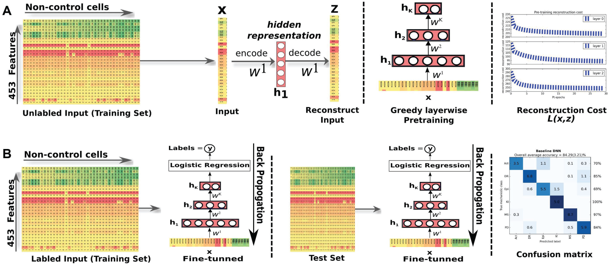
High-content image analysis of breast cancer cells using SAA. (A) Process of unsupervised greedy layerwise pretraining. The features of each cell are encoded into a hidden representation and reconstructed by minimizing reconstruction cost L (x, z). The hidden representation is then used as input for the next layer and the process repeated until the k th hidden layer is completely pretrained. (B) Process of supervised fine-tuning and baseline classifier performance evaluation on the test set.

Framework: Deep Transfer Learning

Traditionally, the goal of transfer learning is to transfer the knowledge (learning) obtained with a source problem to one or more target problems to efficiently develop an effective hypothesis for a new task, problem, or distribution.²⁰

In this work, we combine deep learning with transfer learning by means of a supervised layer-based feature transference^21,22 method. In this method, a deep classifier is obtained (pretrained and fine-tuned) using data from a source problem and reused (partially or not) in the deep classifier for the target problem. The latter is finally fine-tuned with the data from the target problem. By partially, we mean that one can transfer all or part of the source model features (layers) to the target model. In this way, we are transferring knowledge acquired with the source to help in solving the target. It is expected that the TL process supplies the target classifier with an initial set of weights that is a better starting point than the traditional random initialization, providing improved performance (positive transference) over the baseline (by contrast, negative transference occurs when the baseline classifier performs better than the TL classifier). To be more precise, let us introduce some notation considering an SAA with seven hidden layers plus one logistic layer, for both the source and target models. We use four different TL settings for supervised layerwise feature transference. In such settings the 0 represents “no transfer,” that is, the weights of that specific layer of the target model are randomly initialized and not reused from the source model, and the 1 represents “transferred,” that is, the initial weights of that specific layer are obtained (reused) from the trained source model. Note that for each setting, the logistic regression layer is also transferred from the source model to the target model. The setting [00111111] means that we randomly initialized the first and second layers of the target model and transferred all the remaining layers from the source problem. The target network thus built is then fine-tuned with the target data.

LOOCV Training and Network Hyperparameters

Regarding the training process, we followed a procedure similar to that in Ljosa et al.¹⁴ To prevent sharing of batch-specific image properties/features or compound properties between the training and test sets, and thus to prevent the classifiers from learning artifact properties of the set of individual images rather than the more general cell phenotype,²³ we considered using a leave-one-compound-out cross-validation (LOOCV) procedure where all the cells treated with the same compound as the treatment being classified are held out, even if those other cells were treated with a different concentration. Thus, the test set in LOOCV is composed of all the cells from one of the compounds that is held out; the remaining cells (from all the other compounds) are split in a training set, used to train the model, and a validation set, used to prevent overfitting by evaluating early-stopping criteria in the fine-tuning phase. The choice of when to stop fine tuning is based on a geometrically increasing amount of patience. The patience is geometrically increased when the current validation score is below the best validation score. The backpropagation error is fine-tuned until it runs out of patience or the maximum fine-tuning epochs allowed is reached. The trained classifier is then tested on the unseen individual cells from the test set, and each prediction is matched with its ground truth of MOA. The classifier prediction of each cell from the same field of view is then combined to calculate treatment prediction accuracy using majority voting. Each of the experiments is repeated 10 times.

Tuning hyperparameters such as the learning rate or setting the appropriate network architecture for training the deep model is desirable but highly time-consuming. The results of the following section were obtained using SAAs with seven hidden layers of 500 neurons each. We used pretraining and fine-tuning learning rates of 0.001 and 0.1, respectively. The stopping criteria for pretraining were fixed to 60 epochs, which is the value where the reconstruction cost saturates; stopping criteria for fine tuning were set to a maximum of 1000 epochs with the validation set. The complete details of these networks are listed in Supplementary Table S2.

Processing large data as we did, on millions of neural connections, would take several weeks using traditional CPUs. For that reason, we used Theano,²⁴ a GPU-compatible machine learning library, to perform all our experiments on two i7-377 (3.50 GHz), 16 GB RAM with two GTX 770 and five GTX 980 GPU processors, respectively (see High-Performance Computing section of the supplementary material). The software to reproduce the results is available at http://www.deepnets.ineb.up.pt/files/software/DTL_frontend.html.

Results

The analysis of large volumes of multiparametric high-dimensional data without overfitting the network using a high number of cytological features in a time frame suitable for drug discovery presents a significant challenge for any learning algorithm. In the following, we present the results obtained by our approach.

The results of the baseline SAA for classifying MOAs for P_set₁ and P_set₂ datasets are listed in Table 1 . We observe that classifying MOAs of P_set₂ is about 2.8% more accurate than classifying MOAs of P_set₁, even though both datasets have an equal number of MOAs. Also, the computation time to classify the P_set₂ dataset is greater than that of the P_set₁ dataset. The P_set₂ dataset has 61 treatments for 18 compounds, whereas P_set₁ has 42 treatments for 20 compounds. The confusion matrix for classifying MOAs using the baseline approach for both P_set₁ and P_set₂ datasets is shown in Figure 4 , and the precision, recall, and f1-scores are listed in Supplementary Table S3.

Table 1.

Average Accuracy in Percentage and Average Computation Time in Minutes (Standard Deviation in Parentheses) of the Baseline (BL) and DTL Approaches.

Settings					Test		Time per Compound (min)
Approach	Transfer	P _S	P _T	C	Accuracy	p Value (to BL)	Pretrained	Fine-Tuned	Total Time per Repetition (min)
BL			P_set ₁	20	84.29 (3.21)		8.34 (0.0)	16.98 (1.3)	506 (29)
DTL_1	[00000011]	P_set ₂	P_set ₁	20	87.62 (6.96)	0.187	—	17.54 (2.5)	350 (51)
DTL_2	[00001111]	P_set ₂	P_set ₁	20	77.62 (8.80)	0.351		15.08 (1.4)	301 (29)
DTL_3	[00111111]	P_set ₂	P_set ₁	20	86.19 (8.73)	0.589		16.72 (2.0)	334 (41)
DTL_4	[11111111]	P_set ₂	P_set ₁	20	86.43 (3.38)	0.331		10.35 (0.9)	207 (18)
BL			P_set ₂	18	87.05 (4.25)		12.71 (0.2)	26.10 (1.8)	698 (37)
DTL_1	[00000011]	P_set ₁	P_set ₂	18	87.87 (6.86)	0.734		27.36 (2.3)	492 (42)
DTL_2	[00001111]	P_set ₁	P_set ₂	18	69.67 (11.4)	<0.001		21.39 (2.7)	385 (49)
DTL_3	[00111111]	P_set ₁	P_set ₂	18	85.08 (6.99)	0.513		25.33 (2.8)	455 (50)
DTL_4	[11111111]	P_set ₁	P_set ₂	18	75.57 (4.72)	<0.001		19.79 (2.2)	356 (41)

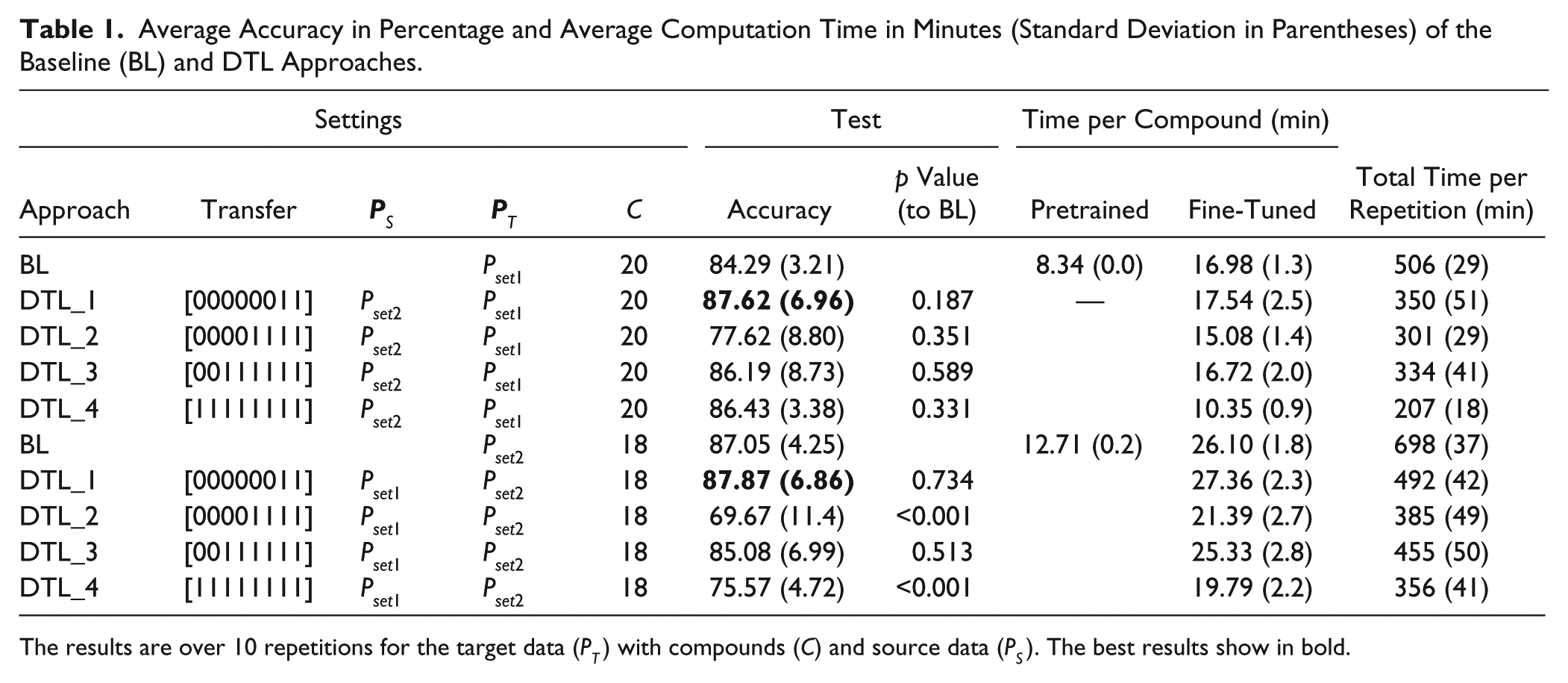
The results are over 10 repetitions for the target data (P_T) with compounds (C) and source data (P_S). The best results show in bold.

To further improve the results over the baseline approach, we considered a deep transfer learning framework where the knowledge gained with the source problem is reused to solve the target problem. The results for four DTL settings are presented in Table 1 and the respective boxplots displayed in Figure 3 . Essentially, we observe that the DTL_1 setting improves over the baseline for both P_set₁ and P_set₂ datasets. It is interesting to note that the best results are obtained when such specific (top) layer weights are transferred from the source to the target problem (the seventh hidden layer weights and the logistic regression weights are reused) and the rest of the (lower) layers are randomly initialized. For example, classifying P_set₁ reusing P_set₂ with the DTL_1 transfer setting produces models 2% more accurate than the baseline and about 0.8% over the transfer all case DTL_4. One of the reasons for this behavior is that higher layers of the network learn problem-specific features from the data, while the lower layers learn generic features;^21-22 thus, it seems beneficial to use the knowledge acquired in the source problem on its higher layers. Moreover, the DTL_1 setting speeds up computation time by 30% over the baseline approach. Confusion matrices for all DTL settings can be analyzed in Figure 4 . Given these results, we believe that DTL_1 would be a good setting to use on similar problems by a researcher who wishes to use DTL on this type of problem.

Figure 3.

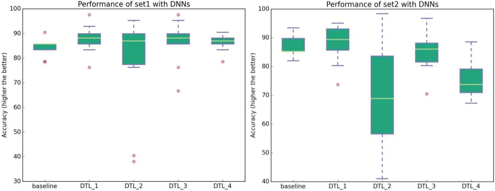
Comparison of baseline vs. DTL approaches. Left: Baseline average accuracy for classifying P_set₁ and DTL approaches for classifying P_set₁ reusing P_set₂. Right: Baseline average accuracy for classifying P_set₂ and DTL approaches for classifying P_set₂ reusing P_set₁.

Figure 4.

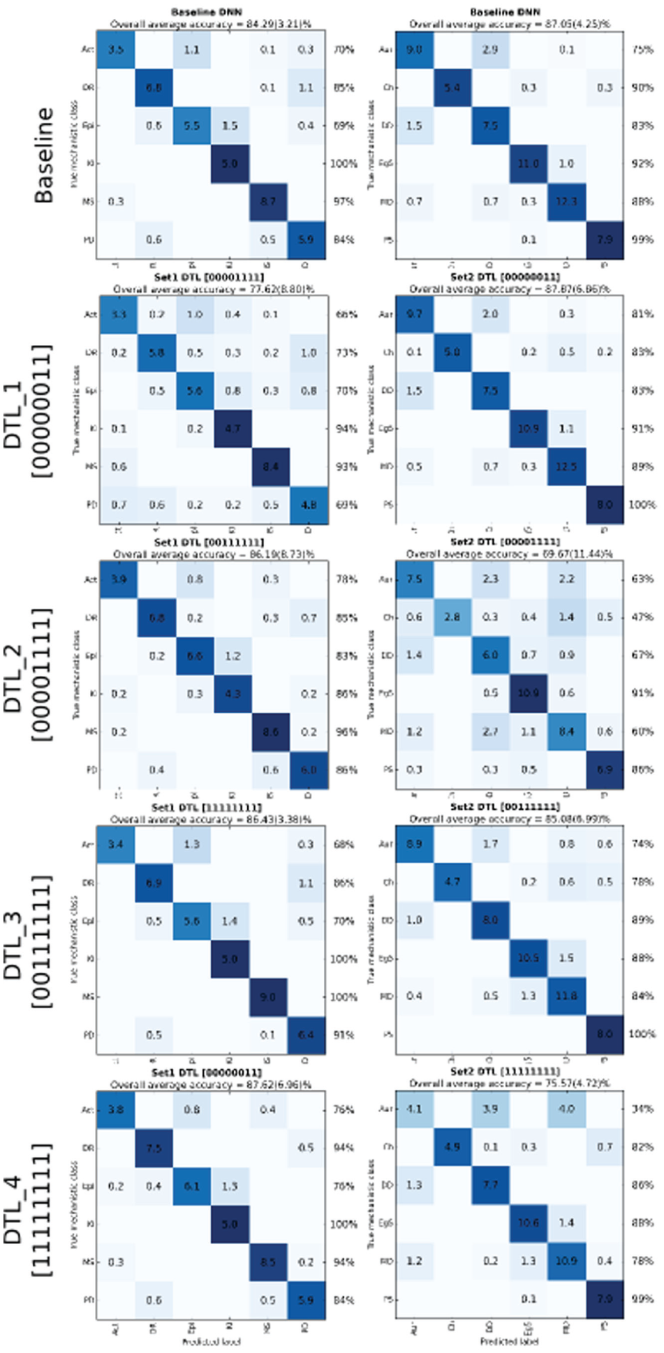
Confusion matrices for the baseline and TL settings on the MOA problem (average outcomes over 10 repetitions). To represent class imbalance, the confusion matrix represents number of elements in each class and the background blue color is normalized confusion matrices (the higher the accuracy, the darker the color).

Comparison with Other State-of-the-Art Methods

Table 2 lists a comparison of our deep learning (baseline and best TL setting) results with two state-of-the-art machine learning algorithms: support vector machines (SVMs)²⁵ with linear and radial basis function (RBF) kernels using a freely available and fast C-based implementation of multiclass SVM (SVM^multiclass, version 2.20). For linear SVM, we optimized the trade-off between training error and margin cost from 0.001 to 50,000 (see Suppl. Table S4), and the best model obtained an overall accuracy of about 21% for P_set₁ and 23% for P_set₂ (see Suppl. Tables S7 and S8). For SVM RBF, we optimized the margin cost from 1 to 1000 and the gamma parameter from 0.001 to 0.00001 (see Suppl. Table S5). As the grid search is computationally expensive, we restricted to only one compound using 10% of the total training data. We observed the best model at margin cost 100 and gamma 0.001, but taking between 419 to 755 min to obtain a 45% accuracy (see Suppl. Table S6). Thus, we performed the experiments with 1% of the total training data to train the SVM RBF and obtained an overall accuracy of about 21% for P_set₁ and 18% for P_set₂ (see Suppl. Tables S9 and S10). Further increasing the number of training samples improves the overall accuracy but leads to a high increase in computation time.

Table 2.

Comparison of Accuracy Obtained and Total Time Taken per Repetition in Minutes with Other State-of-the-Art Methods.

	P_set ₁		P_set ₂
Method	Accuracy (%)	Time (min)	Accuracy (%)	Time (min)
Linear SVM	20.95	32	23.49	49
SVM using RBF (model trained using 1% of total training data)	21.04	78	17.50	125
8-layer-deep architecture (baseline)	84.29	506	87.05	698
DTL_1 [00000011]	87.62	350	87.87	492

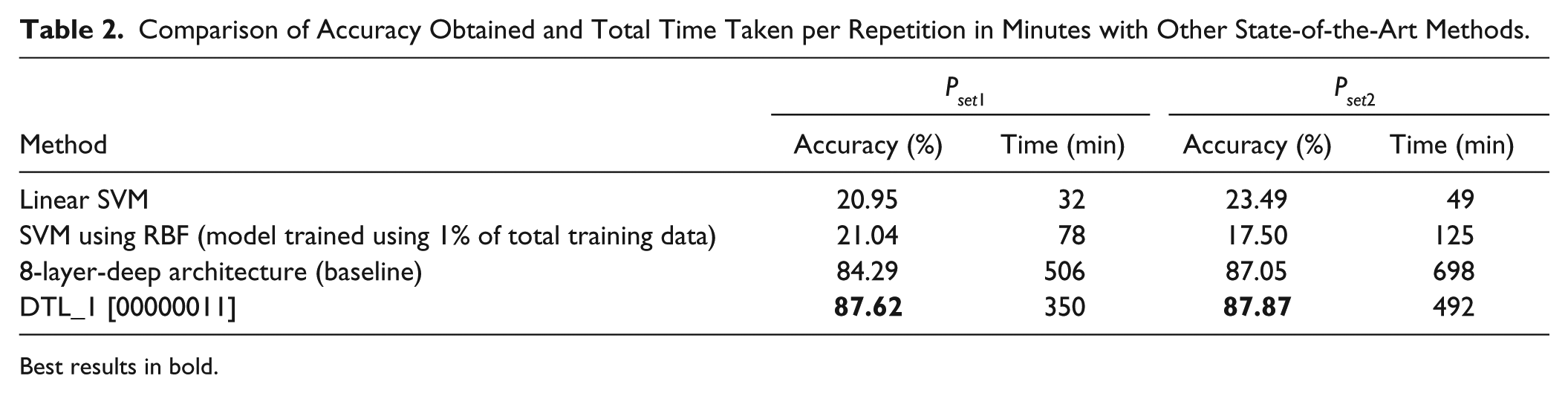
Best results in bold.

Discussion

To stimulate the development of new drugs effective against a wide spectrum of cancers, we propose a deep transfer learning (DTL) classifying framework that uses high-content HCA data. Our classifiers are built upon individual cell information without employing any type of profiling or reduction methods on extracted cell features. The main motivation to use a DTL approach was to show that we can reuse, with minor modifications, the knowledge acquired in solving a given classification problem of MOAs to solve a new one (of MOAs also) without having to follow the whole training procedure. This is particularly useful for new drug testing, as computational time is saved. For that purpose, the data were carefully split into two mutually exclusive six-class problems represented by P_set₁ and P_set₂ datasets. The average accuracies of the baseline SAAs for the P_set₁ and P_set ₂ datasets are about 84% and 87%, respectively, using a seven-hidden-layer SAA with 500 neurons in each layer. The DTL approach showed that the transference of specific weights of the source model was useful, and we have obtained positive transference for both datasets. Although the difference in accuracy of P_set₁ and P_set₂ between baseline and transfer learning is not statistically significant, we observed around 30% computational speedup when using the DTL approach. Our approach was also superior when compared to multiclass support vector machines.

Regarding the 12-class problem, we trained several SAAs ranging from three to eight hidden layers with 500 to 1000 neurons in each layer. However, training a seven-hidden-layer SAA with 500 neurons in each layer may take, on average, 30–48 h per repetition. We performed some preliminary experiments using the adequate leave-one-out approach, and without too much hyperparameter search, the best model obtained around 77% accuracy. As future work, we intend to explore a different approach for the 12-class problem using convolutional neural networks (CNNs) directly applied to the images and not to hand-crafted features. CNNs are state-of-the-art deep neural networks that use a sort of hierarchical representation of the data similar to that of the neocortex and are especially designed for image recognition tasks. We expect to obtain a similar hierarchical feature extraction directly from the images, giving the possibility of the deep network self-extracting relevant cytological features layer by layer.

Footnotes

Acknowledgements

We would like to acknowledge the support of Joaquim Marques de Sá, Jaime S. Cardoso, Vebjorn Ljosa, Shantanu Singh, Szymon Stoma, Tiago Laundos Santos, Jonathan Barber, Ricardo Sousa, and Abhishek Chatterjee. We also acknowledge the valuable comments provided by the reviewers that greatly helped to improve the paper.

Declaration of Conflicting Interests

The authors declared no potential conflicts of interest with respect to the research, authorship, and/or publication of this article.

Funding

The authors disclosed receipt of the following financial support for the research, authorship, and/or publication of this article: This work was financed by FEDER funds through the Programa Operacional Factores de Competitividade—COMPETE and by Portuguese funds through FCT—Fundação para a Ciência e a Tecnologia in the framework of the project PTDC/EIA-EIA/119004/2010.

Supplementary material for this article is available on the Journal of Biomolecular Screening Web site at .

References

Singh

Carpenter

A. E.

Genovesio

Increasing the Content of High-Content Screening: An Overview. J. Biomol. Screen. 2014, 19, 640–650.

LeCun

Bottou

Bengio

. Gradient-Based Learning Applied to Document Recognition. Proc. IEEE 1998, 86, 2278–2324.

Serre

Wolf

Poggio

In Object Recognition with Features Inspired by Visual Cortex, Proceedings of the IEEE Computer Society Conference on Computer Vision and Pattern Recognition, June 20–25, 2005; IEEE: Piscataway, NJ, 2005; Vol. 2, pp 994–1000.

Lee

T. S.

Mumford

Romero

. The Role of the Primary Visual Cortex in Higher Level Vision. Vision Res. 1998, 38, 2429–2454.

LeCun

Bengio

Hinton

Deep Learning. Nature 2015, 521, 436–444.

Schmidhuber

Deep Learning in Neural Networks: An Overview. Neural Netw. 2015, 61, 85–117.

Lee

T. S.

Mumford

Hierarchical Bayesian Inference in the Visual Cortex. J. Opt. Soc. Am. A 2003, 20, 1434–1448.

Bengio

Learning Deep Architectures for AI. Found. Trends Mach. Learn. 2009, 2, 1–127.

Krizhevsky

Sutskever

Hinton

G. E.

In ImageNet Classification with Deep Convolutional Neural Networks, Advances in Neural Information Processing Systems 25—Proceedings of the 26th Conference on Neural Information Processing Systems, Lake Tahoe, NV, Dec 2012; Pereira

Burges

C. J. C.

Bottou

., Eds.; MIT Press: Cambridge, MA, 2012.

10.

Mnih

Kavukcuoglu

Silver

. Human-Level Control through Deep Reinforcement Learning. Nature 2015, 518, 529–533.

11.

Hinton

Deng

. Deep Neural Networks for Acoustic Modeling in Speech Recognition: The Shared Views of Four Research Groups. IEEE Signal Process. Mag. 2012, 29, 82–97.

12.

Sheridan

R. P.

Liaw

. Deep Neural Nets as a Method for Quantitative Structure–Activity Relationships. J. Chem. Inf. Model. 2015, 55, 263–274.

13.

Leung

M. K. K.

Xiong

H. Y.

Lee

L. J.

. Deep Learning of the Tissue-Regulated Splicing Code. Bioinformatics 2014, 30, i121–i129.

14.

Ljosa

Caie

P. D.

ter Horst

. Comparison of Methods for Image-Based Profiling of Cellular Morphological Responses to Small-Molecule Treatment. J. Biomol. Screen. 2013, 18, 1321–1329.

15.

Vincent

Larochelle

Lajoie

. Stacked Denoising Autoencoders: Learning Useful Representations in a Deep Network with a Local Denoising Criterion. J. Mach. Learn. Res. 2010, 11, 3371–3408.

16.

Amaral

Silva

L. M.

Alexandre

L. A.

. In Using Different Cost Functions to Train Stacked Auto-Encoders, Proceedings of the 12th Mexican International Conference on Artificial Intelligence (MICAI), Mexico City, Mexico, Nov 24–30, 2013; Castro

Gelbukh

González

, Eds.; Springer: Berlin, 2013.

17.

Amaral

Sá

Silva

. In Improving Performance on Problems with Few Labelled Data by Reusing Stacked Auto-Encoders, 11th International Conference Image Analysis and Recognition (ICIAR), Vilamoura, Portugal, Oct 22–24, 2014; Campilho

Kamel

, Eds.; Lecture Notes in Computer Science; Springer: Berlin, 2014; Part I, Vol. 8814.

18.

Carpenter

A. E.

Jones

T. R.

Lamprecht

M. R.

. CellProfiler: Image Analysis Software for Identifying and Quantifying Cell Phenotypes. Genome Biol. 2006, 7, R100.

19.

Young

D. W.

Bender

Hoyt

. Integrating High-Content Screening and Ligand-Target Prediction to Identify Mechanism of Action. Nat. Chem. Biol. 2008, 4, 59–68.

20.

Ben-David

Blitzer

Crammer

. A Theory of Learning from Different Domains. Mach. Learn. 2010, 79, 151–175.

21.

Kandaswamy

Silva

L. M.

Alexandre

L. A.

. In Improving Transfer Learning Accuracy by Reusing Stacked Denoising Autoencoders, Artificial Neural Networks and Machine Learning—24th International Conference on Artificial Neural Networks (ICANN), Hamburg, Germany, Sept 15–19, 2014; Wermter

Weber

Duch

., Eds.; Lecture Notes in Computer Science; Springer: Berlin, 2014; Vol. 8681.

22.

Yosinski

Clune

Bengio

. In How Transferable Are Features in Deep Neural Networks? Advances in Neural Information Processing Systems 27—Proceedings of the 28th Conference on Neural Information Processing Systems, Montréal, Dec 8–13, 2014; Ghahramani

Welling

Cortes

, Eds.; MIT Press: Cambridge, MA, 2014.

23.

Shamir

Assessing the Efficacy of Low-Level Image Content Descriptors for Computer-Based Fluorescence Microscopy Image Analysis. J. Microsc. 2011, 243, 284–292.

24.

Bergstra

Breuleux

Bastien

. In Theano: A CPU and GPU Math Expression Compiler, Proceedings of the Python for Scientific Computing Conference (SciPy), Austin, TX, June 20–July 3, 2010; van der Walt

Millman

, Ed.; 2010; Vol. 4: Austin, TX.

25.

Cortes

Vapnik

Support-Vector Networks. Mach. Learn. 1995, 20, 273–297.

26.

Caie

P. D.

Rebecca

E. W

Alexandra

. High-Content Phenotypic Profiling of Drug Response Signatures across Distinct Cancer Cells. Mol. Cancer Ther. 2010, 9, 1913–1926.

Supplementary Material

Please find the following supplemental material available below.

For Open Access articles published under a Creative Commons License, all supplemental material carries the same license as the article it is associated with.

For non-Open Access articles published, all supplemental material carries a non-exclusive license, and permission requests for re-use of supplemental material or any part of supplemental material shall be sent directly to the copyright owner as specified in the copyright notice associated with the article.

0.51 MB

0.00 MB

High-Content Analysis of Breast Cancer Using Single-Cell Deep Transfer Learning

Abstract

Keywords

Introduction

Materials and Methods

Data

Classifier: Stacked Autoassociators

Framework: Deep Transfer Learning

LOOCV Training and Network Hyperparameters

Results

Comparison with Other State-of-the-Art Methods

Discussion

Footnotes

Acknowledgements

Declaration of Conflicting Interests

Funding

References

Supplementary Material