Sage Journals: Discover world-class research

Abstract

The four-parameter logistic Hill equation models the theoretical relationship between inhibitor concentration and response and is used to derive IC₅₀ values as a measure of compound potency. This relationship is the basis for screening strategies that first measure percent inhibition at a single, uniform concentration and then determine IC₅₀ values for compounds above a threshold. In screening practice, however, a “good” correlation between percent inhibition values and IC₅₀ values is not always observed, and in the literature, there seems confusion about what correlation even to expect. We examined the relationship between percent inhibition data and IC₅₀ data in HDAC4 and ENPP2 high-throughput screening (HTS) data sets and compared our findings with a series of numerical simulations that allowed the investigation of the influence of parameters representing different types of uncertainties: variability in the screening concentration (related to solution library and compound characteristics, liquid handling), variations in Hill model parameters (related to interaction of compounds with target, type of assay), and influences of assay data quality parameters (related to assay and experimental design, liquid handling). In the different sensitivity analyses, we found that the typical variations of the actual compound concentrations in existing screening libraries generate the largest contributions to imperfect correlations. Excess variability in the ENPP2 assay above the values of the simulation model can be explained by compound aggregation artifacts.

Keywords

high-throughput screening percent inhibition and IC50 result comparison correlations relationship of primary and dose-response screening results simulation studies sensitivity analysis

Introduction

High-throughput screening (HTS) is typically performed as a stepwise process, starting with a primary screen of compound libraries ranging from 100 000 to 1–2 million compounds at a single concentration. After data normalization, percent inhibition (“activity”) values are obtained for the compounds at the specific screening concentration.^1,2 In a second step, the primary hits (i.e., the compounds passing a fixed threshold or having a larger than 3–6 standard deviation distance from the zero effect level) are selected for concentration-response curve (CRC) validation experiments.^2,3 The determination of an IC₅₀ (“potency”) value is based on fitting the four-parameter logistic Hill equation^4,5 to the data, although more sophisticated models are sometimes used in detailed pharmacological investigations.⁶ The basic assumption of this stepwise HTS design is a reasonable correlation between the percent inhibition and IC₅₀ values, as can be expected from the Hill equation for ideal inhibitors. In screening practice, different sources of variability accumulate and blur this correlation. In addition, in discussion with HTS practitioners, we noticed confusion about what curve such a correlation should be expected to follow. This has led to accounts in the literature where the predictive power of primary, single-concentration screening has been called into question. For instance, McFadyen et al.⁷ at Wyeth describe for a set of 118 compounds a “flat” correlation between percent inhibition data determined in the primary HTS and IC₅₀ values determined in a subsequent step. More dramatically, Spencer⁸ describes the lack of predictive power of primary activity for a set 1200 known actives included in a Pfizer screen. Depending on assay format and quality, primary screening can yield significant numbers of false positives and false negatives. Inglese et al.⁹ have therefore promoted a titration-based approach that they termed quantitative HTS (qHTS), which allows one to confirm hits through replicates and identify CRCs of unusual shape (e.g., bell shaped) directly from primary screening data. With library sizes exceeding 1 million compounds, however, this approach reaches boundaries where logistics, number of data points, and reagent cost become prohibitive. The majority of HTS labs therefore follow the stepwise primary screening model.

Despite these discussions, to our knowledge, the correlation between single-concentration screening data and IC₅₀ values that can be expected both from theoretical considerations, as well as from parameters that influence experimental reality, has not been described in the literature.

We used HTS data sets to examine the correlation between percent inhibition values and IC₅₀ values, using the individual concentrations of the CRC as surrogates for a single concentration experiment. This allowed us to look at the correlation at different concentrations, independent of plate-to-plate and other experimental variability. We then compared these findings with the correlation of CRC results and single-concentration data from the primary screen, thus including all sources of variability one would encounter in real-life screening.

Next, we explored the influence of typical sources of variability, such as compound concentration, on the correlation. To this end, we executed computational simulations to perform a sensitivity analysis of the theoretically expected relationship on the different parameters and to compare the results of these simulations with real-life HTS data.

For the simulations, the general four-parameter logistic Hill equation was used as a definition of the theoretical relationship between percent inhibition data and log₁₀(IC₅₀) data. This allowed investigating the influence of the various Hill curve parameters and also variations in the effective screening concentration and variations in readout scale and data normalization. With these simulations at hand, we were able to explore the boundaries of the current HTS paradigm and essentially derive values for the “best possible” correlations that can be expected given a few basic characteristics of the assay data and of typical compound stock solution libraries. Importantly, we were able to distinguish assays in which the data variability was adequately described by the simulation from types of assays in which additional sources of variability have to be considered. We feel that there is value in clarifying some key relationships in this context, especially since the widespread adoption of screening as a research tool in academia means that scientists will be exposed to these questions beyond a relatively small group of expert users.

Methods

HDAC4 and ENPP2 Assays

The principles and methods of the two assays that are used as illustrations in this article are described in the Supplemental Material.

The Four-Parameter Hill Equation and the Simulations

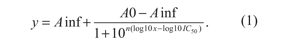
The four-parameter logistic or Hill slope equation (1) is in practice the most frequently used model expression to describe the sigmoid CRCs. It describes the ideal relationship between the inhibition value y at some screening concentration x with a total of four parameters—namely, IC₅₀ (inflection point), the Hill coefficient n (slope), and the asymptotic plateau values A0 and Ainf at low and high concentrations.

y = A \inf + \frac{A 0 - A \inf}{1 + 10^{n (\log 10 x - \log 10 I C_{50})}} .

Several alternative but mathematically equivalent expressions are in practical use.^4,5,10 We have performed Monte Carlo simulation experiments that were designed to obtain a better quantitative understanding of the expected correlation between inhibition values at some constant concentration and the experimentally derived IC₅₀ values from the same experiment (within-curve correlation) and also from independently performed experiments. The latter will mirror the situation encountered when comparing single data point primary screening results with the corresponding IC₅₀ determinations based on different stock solutions or fresh solutions prepared from powder. In most cases, the simulations will represent the “best possible” correlations that can be expected in a screening assay with the same variability as included in the calculations. Uncorrected systematic plate response errors, additional erratic behavior in some assay execution step, or some compound-related distortion effects will increase the observed scatter. A “tighter” correlation of the experimental data than observed in the simulations with given assay quality parameters can occur if the distribution of the effective solution concentration is entered in a too pessimistic way. We think the calculations are useful for the screening practitioner to gain insight into the relationships of the primary percent inhibition results and the IC₅₀ values of the follow-up screen and their possible degree of variation. The simulation studies were all performed using the R statistical computing system.¹¹

In contrast to the standard use of equation (1), we determine the relationship between the inhibition y and log₁₀(IC₅₀) at a certain constant screening concentration x. Due to the symmetry of the equation between the log₁₀(x) and log₁₀(IC₅₀) terms, it is obvious that the relationship between y and the varied factors has a sigmoid shape in both cases.

To perform the simulations in the most realistic way, we base the whole procedure on the generation of suitable “raw data” and subsequent data reduction and data analysis steps in the same way as in a real screening campaign, including normalization and dose-response curve fitting for the derivation of “experimental” IC₅₀ parameters. A graphical outline of the simulation procedure, main parameters, and data-processing steps is shown in Figure 1 .

Figure 1.

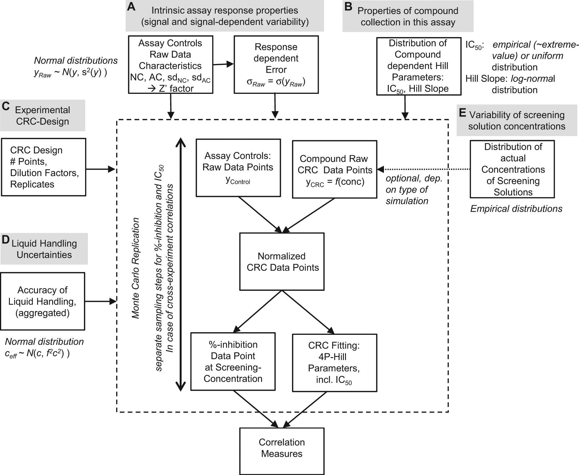
High level overview of the Monte Carlo simulation setup. Experimental factors and simulation parameters A to E are described in more detail in the text and in the Supplemental Material. CRC, concentration-response curve.

The input parameters to the simulation model as outlined in this figure can be categorized as follows: (A) characterization of the raw signal amplitudes y and the signal-dependent uncertainties σ(y) of the various types of control samples, where the continuous response-dependent error is taken as $s^{2} (y) = s_{a}^{2} + s_{b}^{2} \cdot {(y - a)}^{2}$ (similar error laws are often used in analytical chemistry and gene expression analysis^12,13); (B) empirical distribution of the compound-dependent CRC parameters IC₅₀ and Hill slope as an overall representations of the activity properties of the compound collection in the particular assay (see examples in Suppl. Fig. S1); (C) experimental design parameters of the CRC setup (number of concentration points, dilution factors, replicates); (D) accuracy of the liquid-handling equipment; and (E) an optional empirical distribution function describing the effective concentration of screening stock solution libraries found in actual measurements at Pfizer¹⁴ and Novartis (Dollinger, G., unpublished observations). This variation of the effective solution concentration needs to be taken into account when primary screening and CRC validation screening are performed using different compound solutions.

Simulated raw data for controls, percent inhibition, and concentration-response series data are generated in a Monte Carlo procedure, normalized, and fed into a curve-fitting function (R concentration-response curve fitting package “drc”¹⁰) for the estimation of the four parameters of equation (1). These derived parameters are the equivalents of the experimentally derived values, whereas the model input parameters described in (B) above can be considered as the “theoretical” underlying characteristics of the compound effects in the particular assay. The simulation output thus reflects the influence of the different stochastic factors, experimental design aspects, and the CRC parameter estimation procedures. The calculations allow us to assess the influences of the various sources of uncertainties on the correlation parameters. Experimental variability not accounted for in our generic model of common factors of uncertainty in screening processes (e.g., additional compound aggregation effects) will lead to further widening of the distribution and lower the correlation measures accordingly. In this sense, we are able to derive the “highest possible” degree of correlation in the absence of additional “unknown” distortion factors. Further comments and details on data handling in the simulation procedure can be found in the Supplemental Material to this article.

Since the relationship between percent inhibition values and IC₅₀ or log₁₀(IC₅₀) values is nonlinear, as per equation (1), the “usual” linear (Pearson) correlation coefficient¹⁵ should not be used to measure the degree of association. If the data range is restricted to about ±30% around the 50% effect, the approximate linearity of the relationship can still be assumed,¹⁶ but this is no longer the case outside of this range. Examples of the use of the simple linear correlation coefficient over a wide range of concentrations to represent the relationship between inhibition and potency data can be found in the screening literature,¹⁷ but its use is not appropriate. Instead, we use Spearman’s R¹⁸ and Kendall’s τ¹⁹—both characterizing and summarizing monotonic relationships between two variables—and Joe’s δ*,^20,21 an information-theoretical measure for monotonic or nonmonotonic association, as the preferred alternative summaries for association and correlation between our two quantities of interest. δ* is based on the entropy-based mutual information measure but transformed and normalized in such a way that it is equivalent to more “classical” correlations. All these quantities are nonparametric and do not depend on assumed linear relationships. The practical calculation of δ* is based on 2D binning of data, and its value depends to some degree on the number of bins chosen.²¹ We use either a fixed value (n_bin = 10) or n_bin = $\sqrt{K}$ , where k is the total number of data points under consideration. From Kendall’s rank correlation coefficient, we can derive another intuitively understandable quantity of association—namely, the proportion p_τ⁺ of all data point pairs that show a concordant increase in both x and y coordinates of the scatter plot. This quantity is simply given by p_τ⁺ = (τ + 1)/2. The concordance proportion p_τ⁺ can be interpreted as the probability to obtain a consistent activity and IC₅₀ ranking between any two particular data points (compounds) in the analyzed data series. The p_τ⁺ values themselves depend of course on the particular choices for the experimental design and the actual distribution and range of the IC₅₀ values in the assay. The practical calculations of all correlation measures and corresponding significance (p-values) were performed using the bioDist package (http://www.bioconductor.org/packages/release/bioc/html/bioDist.html), which is part of the Bio-conductor software suite.²² Scatter plots displaying the smoothed point density estimate in a color/gray intensity scale provide a very good visual impression of the nonlinear relationship and the extent of the variability of our quantities of interest. The regions of highest point density usually form a “trajectory” following the sigmoid relationship of inhibition and log₁₀(IC₅₀) values. Alternatively, an average smooth trend line for the scatter plots data can be obtained by robust nonparametric smoothing procedures,^23,24 allowing us to visualize the resulting empirical relationships and to calculate the local data variability, that is, the log₁₀(IC₅₀)–dependent standard deviation.²³

It is possible to create an alternative linearized view of the relationship between the initial primary and follow-up CRC experiments by plotting the experimental percent inhibition value and the calculated percent inhibition value at the particular screening concentration using the four Hill equation parameters. This representation has the disadvantage that data points in the transition region around the primary screening concentration, where the variability is usually the largest, are smeared over a wider area of the correlation plot due to the nonlinear nature of the transformation. Furthermore, due to error propagation from the three other Hill equation parameters, the correlation measures can be changed (albeit usually only slightly) by this back-transformation.

Results and Discussion

Observed Experimental Relationships between Percent Inhibition and IC₅₀ Values

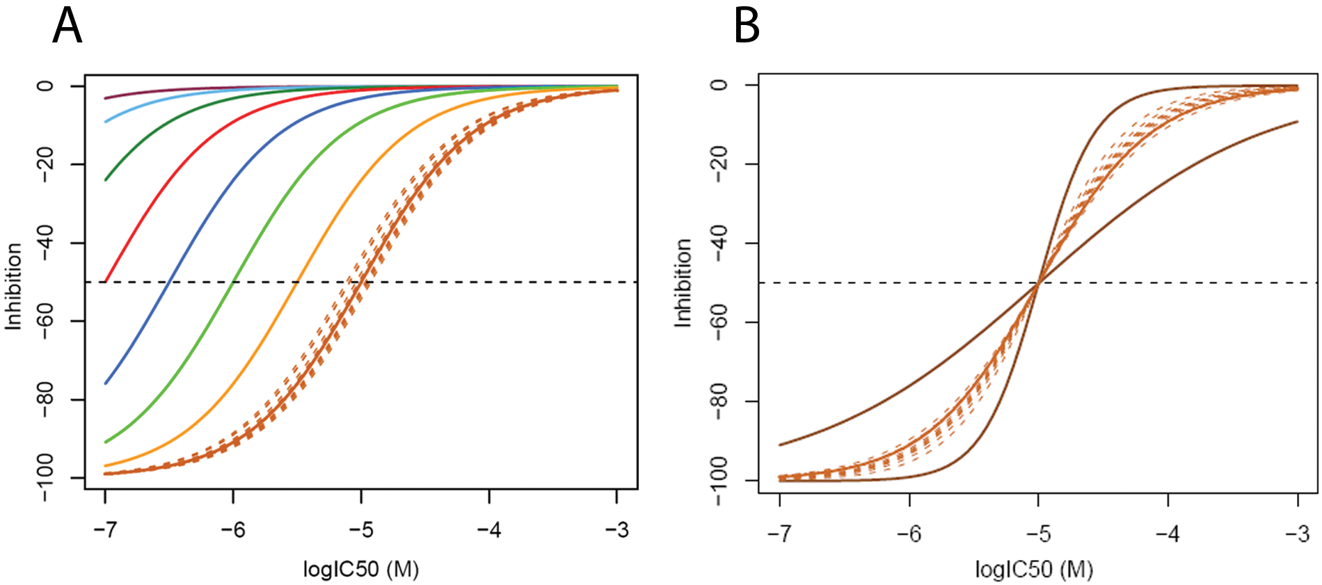
The logistic Hill slope model is used to describe the relationship between a screening concentration and the resulting percent inhibition value. The model, however, can also be used to describe the relationship between an IC₅₀ value and the expected inhibition at a fixed screening concentration. Transformation of equation (1) allowed us to generate Figure 2A , describing the effect of varying the screening concentration from 0.01 to 10 µM for IC₅₀ values ranging from 0.1 µM to 1 mM and assuming A0 = 0 and Ainf = -100 with n = 1. The expected sigmoid relationships are observed, with inflection points at the screening concentration. With decreasing screening concentration, the curves exhibit a left shift, always intersecting the -50% line at the screening concentration. The influence of a possibly varying Hill slope on the given ideal relationship is most pronounced in the region of the bend points¹⁶ of the curves see ( Fig. 2B ).

Figure 2.

(A) Expected relationship between degree of inhibition and log₁₀(IC₅₀) based on logistic Hill slope model. Changing screening concentrations leads to a shift of the curve(s) along the concentration axis (brown = 10 µM, orange = 3.16 µM, green = 1 µM, blue = 0.32 µM, red = 0.1 µM, dark green = 0.032 µM, light blue = 0.01 µM). As an illustration of the influence of typical liquid-handling uncertainties in high-throughput screening, a 15% concentration jitter was added to 10-µM curve. (B) Typical variations of the Hill slope parameter lead to the largest curve differences around the bend points as demonstrated by the center curve with jittered dashed curves around it. More extreme curves with Hill slopes 0.5 and 2 are also shown. The typical variation of the center curve corresponds to the one found in the HDAC4 data.

This sigmoid relationship can be observed in experimental HTS results despite the variation that is associated with such data. Sources of variability in HTS have been reviewed^2,3,25 and include technical errors (instrument malfunction, i.e., pipetting errors), biological errors (i.e., reagent stability and concentration), and statistical errors. We used an enzymatic assay that measured the activity of the histone deacetylase HDAC4. The enzyme removed a trifluoromethyl group from a lysine in a tripeptide substrate. This revealed a trypsin cleavage site, and treatment with trypsin liberated the fluorogenic dye Rh110. Inhibitors of the detection enzyme trypsin were removed in a counterscreen that did not contain HDAC4. However, the impact of compound interference by the choice of a red-shifted fluorogenic dye Rh110 and the removal of nonspecific (e.g., “aggregator”) inhibitors in a counterscreen were designed to minimize the impact of compound interference with the assay.

Of the 3749 compounds that had shown >20% inhibition, 1138 showed >50% inhibition in a 1.4 million primary screen in our test set for this study. Eight concentrations were arrayed in quadruplicates on the same plate to avoid effects from plate-to-plate variability and other random and systematic factors. A total of 1956 compounds did not allow the determination of an IC₅₀ value and were classified as IC₅₀ >10 µM. A further subset of 1283 compounds did not allow the determination of Ainf, or the unconstrained parametric fit failed for other reasons, and therefore the concentration at which the 50% inhibition line was crossed was taken as its IC₅₀ (absolute IC₅₀). The absolute IC₅₀ is a reasonable surrogate value in these cases, as we found a median of 1.02 and a median absolute deviation (MAD) of 0.13 for the ratio of (relative) IC₅₀ to absolute IC₅₀ for the cases where complete curves were obtained. The remaining 510 compounds allowed a fully unconstrained parametric fit to the Hill equation, with IC₅₀ values ranging from 7 nM to 10 µM. Overall, we have obtained 785 IC₅₀ values from the complete primary hit list (20% inhibition cutoff) and 656 IC₅₀ values for compounds initially exhibiting more than 50% inhibition, which corresponds to a 58% validation rate of this set of primary hits.

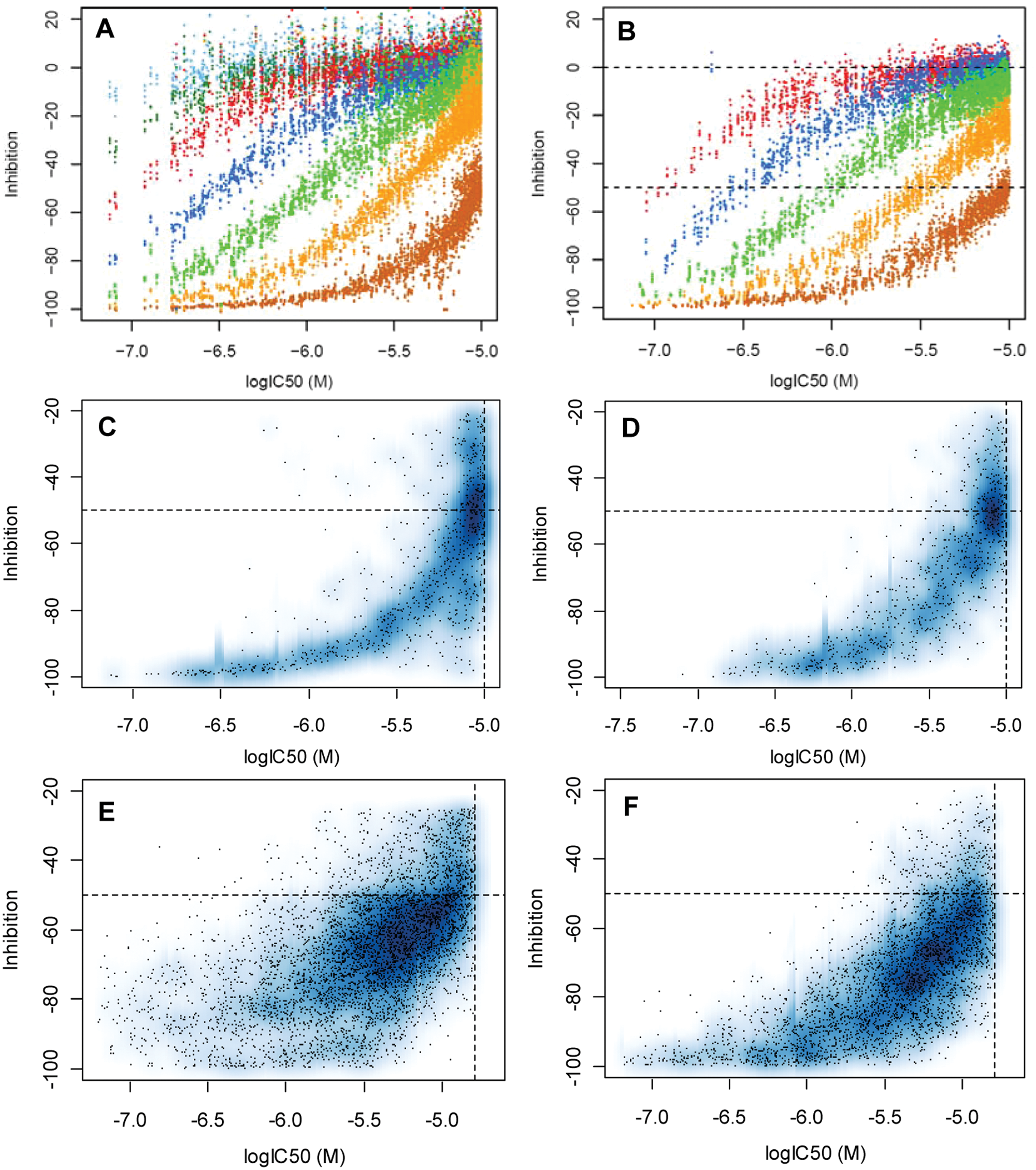
In Figure 3A , the measured CRC inhibition values were plotted against the log₁₀(IC₅₀) value for all concentration points, so this plot shows the within-curve relationships of these quantities.

Figure 3.

(A) Experimental within-curve correlation scatter plot of the HDCA4 assay derived from the individual concentrations of the dose-response experiment. Data were measured in quadruplicates, and all data points are plotted. The color coding is the same as in Figure 2A . (B) Illustration of the within-curve relationship of simulated percent inhibition (quadruplicates) and fitted IC₅₀ values based on characteristic simulation parameters that are equivalent to the HDAC4 assay, Z′ = 0.86. Color coding for the different screening concentrations is the same as in Figure 2A . Calculations for x = 0.1 to 10 µM. (C) Experimental percent inhibition-log₁₀(IC₅₀) scatter plot of HDAC4 assay data from the two different experimental phases. Primary inhibition data measured at 10 µM. (D) Simulated data for independent inhibition and IC₅₀ determinations with assay quality parameters as for the real HDAC4 assay and added factor for differences in effective screening concentrations. (E) Experimental percent inhibition-log₁₀(IC₅₀) scatter plot of ENPP2 assay data from the two different experimental phases. Primary inhibition data measured at 16 µM. (F) Simulated data for independent inhibition and IC₅₀ determinations with assay quality parameters as for the real ENPP2 assay and added factor for differences in effective screening concentrations. The vertical dashed lines in C–F are placed at the respective primary screening concentration value.

The equivalent relationship can also be observed in a “real-life” screening situation, that is, by plotting the percent inhibition values obtained during primary screening against the IC₅₀ values ( Fig. 3C ). The spread of the data increased, especially for lower potency compounds, and the sigmoid relationship is truncated by the highest concentration of the CRC, as well as by the cutoff at 20% inhibition that was used for hit selection in the primary screen. As expected, the region of highest point density passes through -50% at the primary screening concentration of 10 µM.

A semi-logarithmic plot as in Figure 3C allows an immediate judgment on a question that is frequently asked by project teams—that is, if the IC₅₀ values are in accordance with the primary screening data and if the primary screen is predictive of compound potencies as measured in the IC₅₀ experiment. A simple plot as used and proposed here gives immediate confidence in the data quality but, to the best of our knowledge, has so far not been used in literature to give a visual and very intuitive representation of the relationship of the main results of a typical HTS campaign.

Clearly, values will often deviate from the ideal sigmoid curve in real screening data. Differences in compound concentrations, Hill slope values other than 1, and many other factors can affect the correlation. To understand the influence of the major different sources of variability, we built a phenomenological mathematical model that allows the determination of the influence of the most important assay characteristics and parameters on the correlation.

Calculated Relationships between Percent Inhibition and IC₅₀ Values

The computational experiments allow us to perform a quantification of the expected relationship and variability between single-point inhibition data and estimated IC₅₀ values. A quantification of the relationships (joint or conditional parameter density distributions, correlation summaries) from the simulation results is easily accomplished. Also, rough estimates of expected false-negative and false-positive probabilities for single-point primary data, based on a fixed inhibition threshold (e.g., 50%) and on an upper limit setting on the empirical compound potency in the validation screen (e.g., 10 µM), can be made. In actual screening situations, factors that are not taken into account in the simulations might come into play and modify the overall picture somewhat.

An underlying assumption in the simulation procedure for “separate experiment” runs is that the assay quality in the single-point primary screen is the same as in the serial dilution validation screen. The results derived from such simulation studies are usually “best-case” results under the assumptions mentioned above, but as such they are valuable for getting more quantitative insight into the highest possible degree of correlation that can be expected between primary and validation experiments in an assay with a particular design (concentration range, number of replicates, number of concentrations), quality characteristics (dynamic signal range and assay error law, indirectly measured by Z′ factor), process-related factors (concentration variability, liquid-handling reproducibility/variability), and finally also the range and distribution of IC₅₀ values in the assay.

In Figure 3B , we show the within-curve correlation plots of the simulated data based on the key characteristics of the actual HDAC4 screen that can be compared with the experimental situation as displayed in Figure 3A .

The resulting within-curve correlation of the simulated and the actual assay data at 10 µM with the respective fitted IC₅₀ values is shown in Table 1 . The ranges of values are derived from 10 independent repetitions of the simulation runs. In addition, as previously described, the δ* values also depend on the number of data bins chosen for the calculations.

Table 1.

Comparison of Correlation Measures for the Within-Curve (Same Experiment) Relationship between Inhibition and log₁₀(IC₅₀) Values at 10 µM Screening Concentration

	Spearman R	Kendall τ	Concordance Proportion p_τ+	δ* Mutual Information	Figure
HDAC4 Assay (Z′ = 0.86)	0.83	0.63	0.82	0.83–0.89	3A
Simulation (Z′ = 0.86)	0.90–0.93	0.75–0.79	0.88–0.90	0.90–0.95	3B, 4C
Simulation (Z′ = 0.4)	0.81–0.85	0.62–0.68	0.81–0.84	0.85–0.94	4D

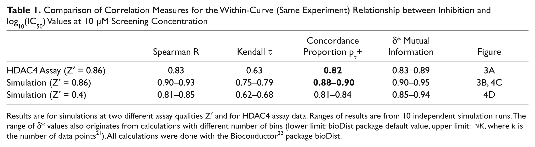
Results are for simulations at two different assay qualities Z′ and for HDAC4 assay data. Ranges of results are from 10 independent simulation runs. The range of δ* values also originates from calculations with different number of bins (lower limit: bioDist package default value, upper limit: $\sqrt{K}$ , where k is the number of data points²¹). All calculations were done with the Bioconductor²² package bioDist.

We observe that the different experimental within-curve correlation measures are slightly smaller than the results of simulation runs with the Z′ = 0.86 parameters, but in both cases, the sigmoid relationship (right-truncated at the screening concentration) is clearly discernible, and the correlation measures are all highly significant (p < 10⁻¹⁶). When comparing Figure 3A and 3B , we can see that at 10 µM (brown data), a slightly higher fraction of HDAC4 assay data points lies further away from the bulk of the sigmoid-shaped distribution than is the case for the simulated data set. Such “outliers” are not captured and modeled in the present simulation setup. Often, groups of two or more points of a quadruplicate are outliers in this sense, and this then leads to the observed lowering of the correlation measures. We have not incorporated such “systematic” errors (i.e., comprising whole groups of data points) and outlier contributions in our simulations because too many ad hoc tuning parameters would have been needed, and our primary aim was to represent the main characteristics of a reasonably well-behaved assay setup and the resulting percent inhibition-log₁₀(IC₅₀) relationships in an approximate quantitative way.

The data in Figure 3D were calculated with the same characteristics as the (10 µM, brown) data in Figure 3B , but an additional factor—namely, a probability distribution that describes the possible differences between the effective screening solution concentrations in the primary and validation runs—was introduced.¹⁴ The corresponding correlation measures are shown in Table 2 . When comparing Figure 3C and 3D , we observe that the most prominent part of the experimental relationship (left) is more discernible (has higher point density) and less “washed out” than in the simulated correlation plot (right). On the other hand, a slightly wider small background distribution is observed in Figure 3C . Possible explanations for these differences are the following: (1) The ratio of the effective concentration between primary and validation runs is less random and more highly correlated (i.e., likely more compound dependent) than what sampling from the empirical distribution derived from a broad range of different compounds suggests,¹⁴ and (2) uncontrolled and random experimental factors (e.g., differences in assay reagent batches, occasional differences in reagent stability, changes in the dynamic range of responses, changes in liquid handler calibrations and stability, and dropouts of single pipettor needles) that we already had observed in Figure 3A to some degree may play an even larger role in the primary screening situation than in the validation screen and the corresponding within-curve relationship. Clear outliers and possibly resulting bad curve fits are more easily detectable in the IC₅₀ estimation phase, and such data or curves will more likely be eliminated, whereas this is not possible in nonreplicated primary screening. In this sense, the final IC₅₀ result collection is much less influenced by remaining random experimental variations than the single primary inhibition data. Nonetheless, in reasonably well-behaved and quality-controlled assay runs, this should not be a large problem.

Table 2.

Comparison of Correlation Measures for the Relationship between Inhibition and log₁₀(IC₅₀) Values at 10 µM Screening Concentration for Independent Experiments

	Spearman R	Kendall τ	Concordance Proportion p_τ+	δ* Mutual Information	Fig.
HDAC4 Assay (Z′ = 0.86)	0.73	0.57	0.79	0.79–0.90	3C
Simulation (Z′ = 0.86)	0.81–0.84	0.60–0.65	0.80–0.83	0.82–0.90	3D, 4A
Simulation (Z′ = 0.4)	0.74–0.77	0.54–0.58	0.77–0.79	0.78–0.84	4B
Simulation (Z′ = 0.4, IC₅₀ range restricted to interval 1–10 µM)	0.62–0.66	0.43–0.48	0.72–0.74	0.61–0.82
ENPP2 assay (Z′ = 0.82)	0.6	0.42	0.71	0.60–0.82	3E
Simulation (Z′ = 0.82)	0.74–0.77	0.55–0.57	0.77–0.78	0.73–0.87	3F

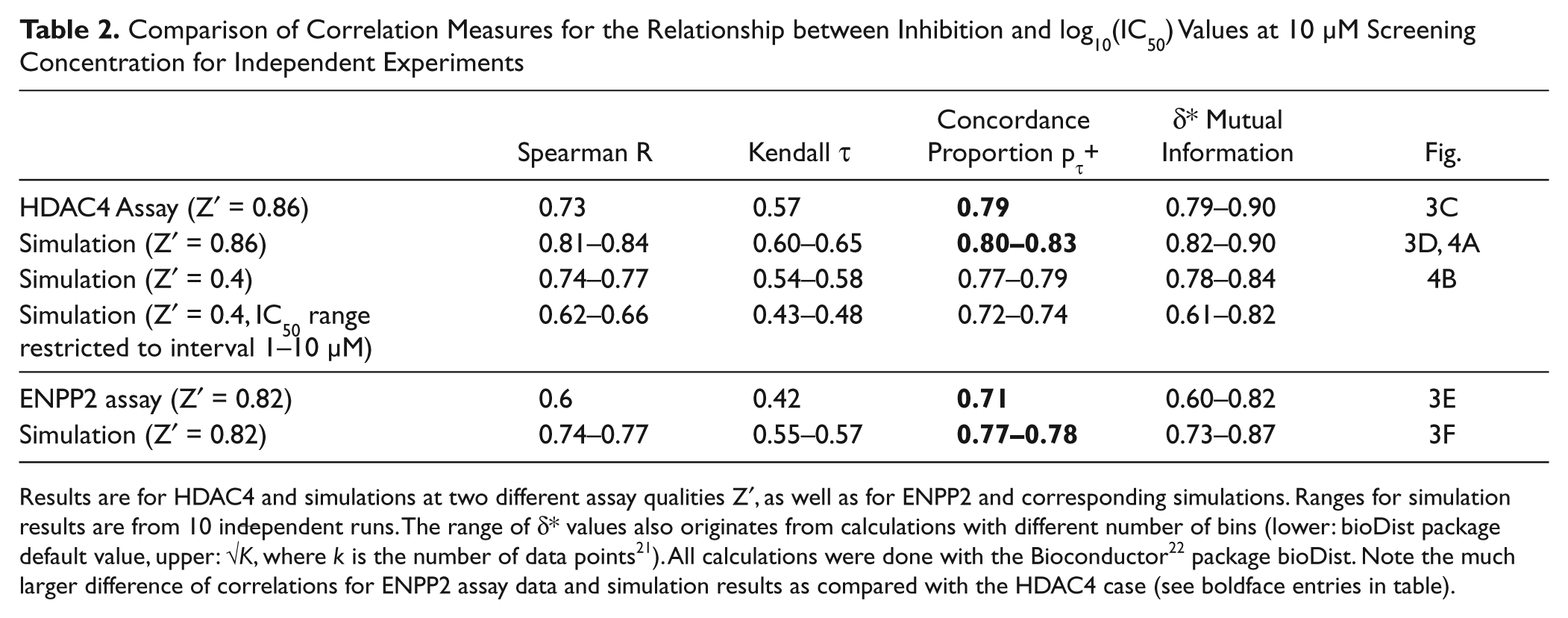
Results are for HDAC4 and simulations at two different assay qualities Z′, as well as for ENPP2 and corresponding simulations. Ranges for simulation results are from 10 independent runs. The range of δ* values also originates from calculations with different number of bins (lower: bioDist package default value, upper: $\sqrt{K}$ , where k is the number of data points²¹). All calculations were done with the Bioconductor²² package bioDist. Note the much larger difference of correlations for ENPP2 assay data and simulation results as compared with the HDAC4 case (see boldface entries in table).

Similar to the previous within-curve correlation coefficients, we observe here also somewhat smaller values for the actual assay data than for the corresponding simulation with Z′ = 0.86. As previously discussed, the slightly broader background in the real assay data ( Fig. 3C ) as compared with the simulation ( Fig. 3D ) is not completely surprising. So it is again the comparatively larger set of “outlier” data that lowers the degree of association and concordance in the HDAC4 data. It is easy to show, for example, that a 10% random contamination (a homogeneous background of random inhibition values) of a data set with the same characteristics as our Z′ = 0.86 example with τ = 0.7, p_τ⁺ = 0.85 will lower these values to approximately τ = 0.6, p_τ⁺ = 0.8 and exhibit similar shifts for the other correlation measures. From τ = 0.6, p_τ⁺ = 0.80, the reduction is on average down to τ = 0.55, p_τ⁺ = 0.78, so roughly what we observe as shifts between the “optimistic” Z′ = 0.86 simulation and the actual assay data for the within-curve correlations ( Table 1 ) and for independent experiments ( Table 2 ), respectively.

The general assay data quality characteristic can be derived more directly than the solution concentration differences between the single-point and the concentration-response screens. The latter can be accommodated in an average and approximate way by integrating historical information on the distribution of the effective concentrations of screening solutions into the calculation. Other random factors leading to “outlier” data can be considered in a summary fashion, as mentioned in the previous paragraph. Both these “noise” contributions will lead to some degree of lowering of the correlation measures. Because both of these phenomenological factors cannot be determined experimentally in the context of a particular assay (for purely practical and economic reasons), we are taking them into account via the described summary approaches (empirical concentration distributions and estimates of correlation reduction factors in the presence of “background” noise).

In summary, a comparison of experimental and simulated data ( Fig. 3C , D ) showed that typical data characteristics of HTS experiments combined with factors such as concentration variation of stock solutions were sufficient to account for the observed data variability. For several other biochemical assays, we see similar degrees of agreement of primary and secondary IC₅₀ screening results (data not shown), and we can conclude that the main factors of variability in HTS experiments are captured by our procedure.

A similar data set from an ENPP2 screen was analyzed as an example for a more challenging assay ( Fig. 3E , F ). The assay is based on cleavage of the quenched substrate FS-3. FS-3 is an analogue of the endogenous substrate lysophosphatidylcholine (LPC).^26,27 During assay development, we found the assay to be quite sensitive to compound aggregation, which could partially be controlled by addition of detergents in the assay buffer (see Supplemental Material). A primary screen of 1.4 million compounds was run with a Z′ factor of 0.82, and after a confirmation run, 5262 compounds were selected for IC₅₀ determination. To minimize interference by fluorescent compounds, we determined IC₅₀ values from slope changes of reaction progress curves rather than from end-point measurements. The experimental data set in Figure 3E and the corresponding simulated experiments in Figure 3F clearly show that in this case, sources of data variability are at play that are not included in the basic simulation. These factors are likely assay specific, and in this case, compound aggregation and readout differences between the primary end-point format and the kinetic measurement format for the IC₅₀ determination phase are likely causes for the discrepancy.

In Figure 4 , we show a set of scatter plots to compare the general appearance of the calculated inhibition-log₁₀(IC₅₀) relationship based on HDAC4 assay data characteristics but varying Z′ for the two cases of independent experiments and within-curve correlations. The corresponding correlation measures are shown in Tables 1 and 2 . The Z′ = 0.4 example case ( Fig. 4B , D ) corresponds to a 4.5-fold increase of the standard deviations of the controls as compared with the simulated data set with Z′ = 0.86 ( Fig. 4A , C ). We can see that the influence of the inclusion of the differences in the effective screening concentration ( Fig. 4A , B ) is visually dominating the scatter plot (wider scattering of data), much above the effect of the change in assay data quality. This contrast in appearance is also reflected in the larger average difference of the correlation measures between the different types of experiments (i.e., between Tables 1 and 2 or between the upper and lower rows of plots in Fig. 4 ) than is found between the different Z′ values (i.e., between left and right plots in Fig. 4 ). The contrast difference is most pronounced in δ* when taking the upper value range limits (which are calculated with the “optimal” number of bins) because the mutual information measure²¹ is estimated from the occupation numbers of the 2D scatter plot (2D histogram) and thus quite directly related to its visual appearance.

Figure 4.

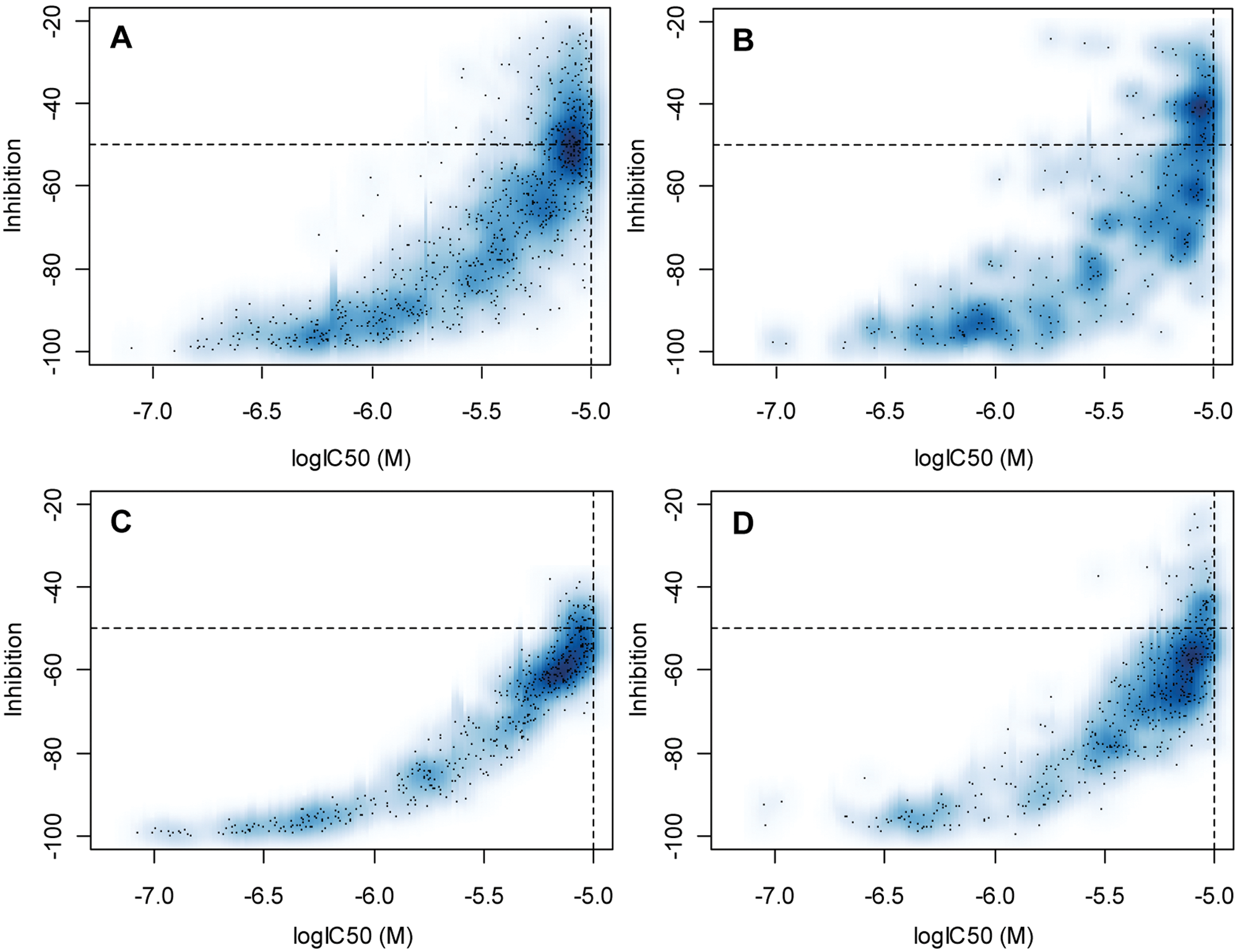
Illustration of the simulated inhibition-log₁₀(IC₅₀) relationships in independent and identical experiments with varying assay quality. For the independent experiments, the effective screening concentration for inhibition and IC₅₀ determinations was independently varied based on empirical solution concentration distributions. (A) Independent experiments, Z′ = 0.86. (B) Independent experiments, Z′ = 0.4. (C) Identical experiments, within-curve correlation, Z′ = 0.86. (D) Identical experiments, within-curve correlation, Z′ = 0.4.

When looking at a more restricted range of IC₅₀ values, the correlation measures will naturally tend to become smaller, as for any underlying increasing relationship between two quantities. We show an example of this effect for the Z′ = 0.4 simulation results in Table 2 . When only considering the IC₅₀ range from 1 to 10 µM (half the initial logarithmic data range), then all correlation values become considerably smaller, but the corresponding p-values are still <10⁻¹⁶, and thus all correlations continue to be statistically highly significant also for the smaller data range.

A more extensive comparison of correlation data with the basic HDAC4 characteristics but varying assay data quality (Z′ factor) and the influence of the solution concentration uncertainties is shown in Figure 5 .

Figure 5.

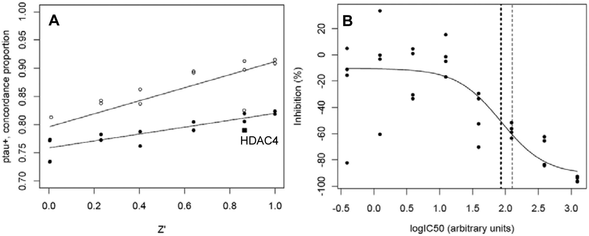
Illustration of the dependence of correlation measures on assay data quality (Z′ factor). The concordance proportion p_τ⁺ can be interpreted as the probability of preserving the activity rank order between any two pairs of data points in the inhibition versus IC₅₀ scatterplots. (A) p_τ⁺ dependence on Z′ for independent experiments with empirical solution concentration variation (filled circles) and without solution concentration variation (open circles). Results are from two independent simulation runs at each selected Z′ value. A pipetting uncertainty factor of 10% was always added in the simulated data, resulting in the lowering of the Z′ = 1 data points from 1 (expected ideal correlation, respectively, from 0.96 when still allowing a variation in the Hill slope values) down to 0.91 for the second result set. Lines are added to guide the eye. The actual HDAC4 assay data point is shown as a filled square (see also Table 2 ). The results are of course dependent on the particular experimental design (quadruplicate data points at eight concentrations with two dilution steps per decade) and distribution and range of actual IC₅₀ values. (B) Randomly picked simulated example concentration-response curve (CRC) data set and curve fit example with assay Z′ factor of 0, showing that a seemingly “unusable” assay still can produce interpretable concentration-response relationships. The data point replications and measurements at multiple concentrations effectively offset the scatter exhibited by individual data points. The theoretical model IC₅₀ is marked by the thin dashed vertical line and the resulting “experimental” IC₅₀ based on the simulated data and subsequent Hill curve parameter estimation by the thicker vertical line.

We have performed a series of simulation experiments with varying Z′ factor for two different situations—namely, with and without inclusion of the solution concentration distribution factor. Both result sets are shown in Figure 5A . A particular Z′ factor can be generated by multiple differently sized standard deviation (SD) values of the two types of controls when their respective means are constant. In the calculations, we have chosen to proportionally increase both control SD values, and for the Z′ = 0 case, we have also explored the more extreme “symmetric” error situation where the SD value of both controls is equal in size. This creates a wider distribution for values with “full inhibition” and then results in the lower p_τ⁺ value for both types of relationships shown in Figure 5A . We again observe highly significant correlations between primary and IC₅₀ data for this much wider range of the Z′ data quality indicator than we have previously shown in Tables 1 and 2 .

In Figure 5B , we show an arbitrary example of a simulated CRC data set, which was generated with the asymmetric control error distribution resulting in Z′ = 0. Curve fitting and the derivation of reasonably accurate IC₅₀ values (as judged by the two vertical IC₅₀ markers for model value and “experimental” result) are still possible even with such “low” data quality because of replicated measurements and the presence of data at multiple different concentrations. This will largely offset the uncertainties of single data points in the CRC data.

Another type of calculation allows us to determine the likely variation of inhibition values in different regions of activity values. These simulations are based on a uniform distribution of log₁₀(IC₅₀) values over a larger numerical range than in the previous calculations. An example of such a calculation (IC₅₀ range from 0.1 µM to 1 mM, 10 µM primary screening concentration) using the same basic system parameters as used for the ones in Figure 3D or Figure 4A is shown in Figure 6A .

The smooth local regression line provides the basis for calculating the approximate standard deviation. The individual absolute values of residuals based on the local regression curve are shown in Figure 6B . They allow the derivation of a smooth estimate for the locally varying median absolute residuals and, subsequently, a robust standard deviation measure.²³ The line in Figure 6B represents this varying standard deviation. The asymmetry in the curve position between strong inhibitors (left) and inactive compounds (right) is clearly visible. This is a direct reflection of the respective response variability of the full-inhibition and zero-effect controls or samples, respectively. The significantly larger variability for samples with an IC₅₀ around the screening concentration is readily visible and reaches the 4- to 5-fold value of the zero-effect samples. A concomitant strong increase in false-positive and false-negative rates for samples with such “borderline” potencies above estimates that are based only on control sample response variability is obvious. The increase of the error in the center region is of course related to the rate of change of the inhibition-log₁₀(IC₅₀) relationship—largest around the inflection point—and is expected on these grounds, but the simulation allows us to provide a rough quantification of the increase due to factors that are not directly tractable through a formal mathematical analysis, which is simply based on equation (1).

Figure 6.

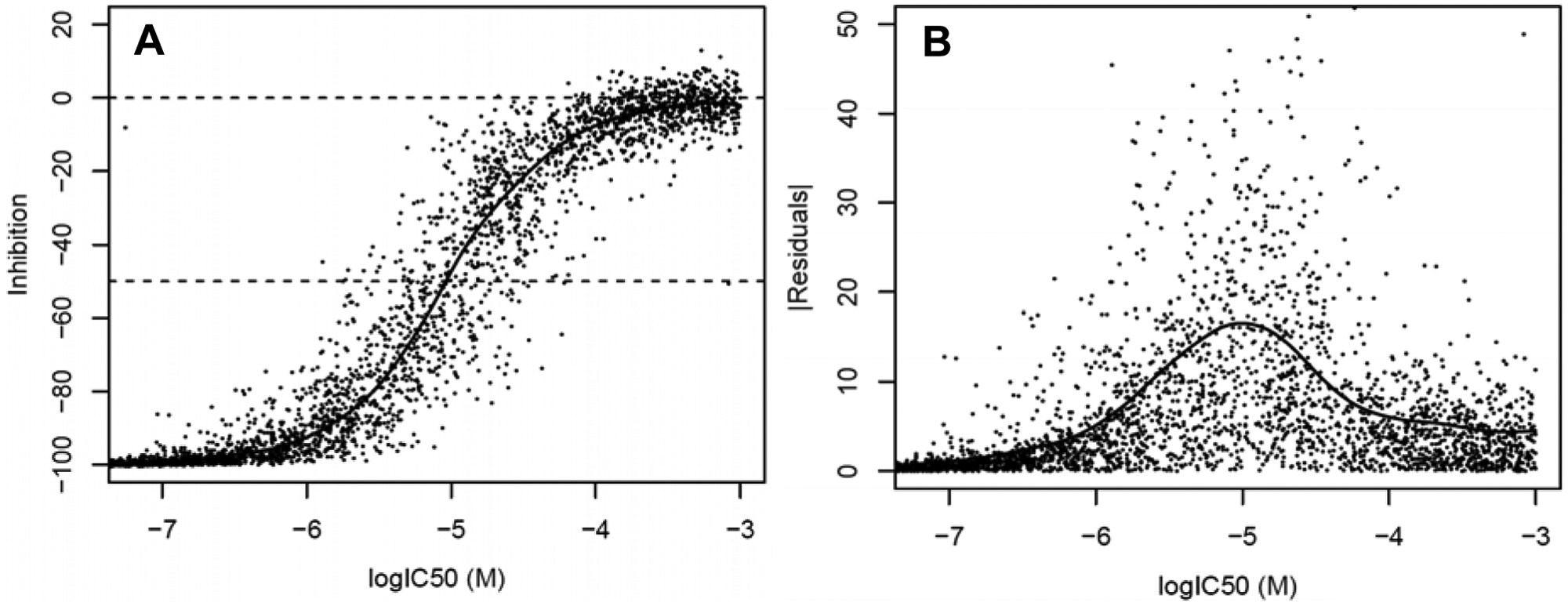
Illustration of the relative increase of percent inhibition variability for values between the bend points of the nominal theoretical relationship based on equation (1). (A) Simulated data from independent experiments (cf. Fig. 4D) and percent inhibition-log₁₀(IC₅₀) correlation at a 10-µM screening concentration for a wider range of IC₅₀ values (0.1 µM to 1mM), so including values way above 10 µM. Basic assay quality characteristics are set according to the HDAC4 case. (B) Absolute residuals of data points with respect to the local regression line in A. The full curve is the locally varying (robust) standard deviation, as calculated from the absolute residuals.²³

The question of whether primary screening data are predictive of IC₅₀ values is encountered frequently in lead-finding projects. Through a transformation of the Hill equation, we have generated plots that show the correlation of percent inhibition values with IC₅₀ values under ideal conditions. Using an example of a typical biochemical assay of HDAC4 activity, we were then able to show that this ideal behavior can be observed under real screening conditions, despite the many factors that contribute to data variability in screening data. We then moved on to examining the influence of typical sources of data variability on the quality of the percent inhibition versus IC₅₀ correlation. Building a mathematical simulation that models the influence of experimental sources of variability, we found that choosing typical values for distribution of compound concentration, statistical assay quality, and distribution of Hill coefficients, for example, resulted in result distributions that are very similar to the experimental data. This confirms that these common factors are largely sufficient to explain variability in experimental data that is observed, for example, in the HDAC4 assay, which possesses a good statistical quality (Z′ = 0.86).

In addition to sources of variability that are common to all screens, there may be sources of variability that are assay specific. For example, the influence of non-stoichiometric inhibition through compound aggregation is highly buffer dependent. In a second example of an ENPP2 screen, these factors resulted in a noticeable discrepancy between the experimental and the simulated data. It should be noted that this discrepancy is not reflected in the statistical quality of the ENPP2 assay as described by Z′ = 0.82.

In an attempt to quantify the deviation from ideal behavior for experimental data, we calculated different correlation coefficients. These coefficients allow judging the relative influence of different sources of data variability. We have found that the distribution of compound concentration in screening decks is the largest single common contributor to data variability in an HTS setting and influences the variability of primary screening data stronger than the assay quality measured by the Z′ factor. In addition, the correlation coefficients, together with the plots, allow researchers to spot assays that are influenced by assay-specific sources of variability, in addition to the general boundary conditions of the HTS experiment, which are mirrored by the simulation results. Derived in pilot screening, they may be useful in triggering additional efforts in assay development.

In this contribution, we hope to provide lead-finding scientists with a practical framework to discuss and judge the predictiveness of their primary screening data. As we find adequately large correlation measures even for the more problematic assay that we have investigated (p_τ⁺ > 0.7), we conclude that for robust assays with good Z′ factors, the HTS paradigm of single-concentration screening followed by concentration-response curves is a valid and cost-efficient approach to detect active compounds and compound families.

Footnotes

Acknowledgements

Drs. Peter Fürst and Adam W. Hill are acknowledged for various discussions and support. We thank Sandrine Ferrand, Aline Tirat-Boeuf, and Lukas Leder for experimental work. We also thank the anonymous reviewers for their comments and some suggestions for improvement.

Declaration of Conflicting Interests

The authors declared no potential conflicts of interest with respect to the research, authorship, and/or publication of this article.

Funding

The authors received no financial support for the research, authorship, and/or publication of this article.

Supplementary material for this article is available on the Journal of Biomolecular Screening Web site at .

References

Hüser

Lohmann

Kalthof

Burkhardt

Brueggemeier

High-Throughput Screening for Targeted Lead Discovery. In High-throughput Screening for Lead Discovery; Hüser

, Ed.; Wiley-VCH: Weinheim, Germany, 2006; pp. 15–36.

Malo

Hanley

J. A.

Cerquozzi

Pelletier

Nadon

Statistical Practice in High-Throughput Screening Data Analysis. Nat. Biotechnol. 2006, 24, 167–175.

Coma

Herranz

Martin

Statistics and Decision Making in High-Throughput Screening. In High-Throughput Screening, Methods and Protocols; Janzen

W. P.

Bernasconi

, Eds.; Humana Press: Totowa, NJ, 2009; pp. 69–106.

De Lean

Munson

P. J.

Rodbard

Simultaneous Analysis of Families of Sigmoidal Curves: Applications to Bioassay, Radioligand Assay, and Physiological Dose Response Curves. Am. J. Physiol. 1978, 235, E97–E102.

Fomenko

Durst

Balaban

Robust Regression for High Throughput Drug Screening. Comput. Methods Programs Biomed. 2006, 82, 31–37.

Gottschalk

P. G.

Dunn

J. R.

The Five-Parameter Logistic: A Characterization and Comparison with the Four-Parameter Logistic. Anal. Biochem. 2005, 343, 54–65.

McFadyen

Walker

Alvarez

Enhancing High Quality and Diversity within Assay Throughput Constraints. In Chemoinformatics in Drug Discovery; Oprea

T. I.

, Ed.; Wiley-VCH: Weinheim, Germany, 2004; pp. 143–173.

Spencer

R. W.

High-throughput Screening of Historic Collections: Observations on File Size, Biological Targets, and File Diversity. Biotechnol. Bioeng. (Comb. Chem.). 1998, 61, 61–67.

Inglese

Auld

D. S.

Jadhav

Johnson

R. L.

Simeonov

Yasgar

Zheng

Austin

C. P.

Quantitative High-Throughput Screening: A Titration-Based Approach That Efficiently Identifies Biological Activities in Large Chemical Libraries. Proc. Natl. Acad. Sci. U. S. A. 2006, 103, 11473–11478.

10.

Ritz

Streibig

J. C.

Bioassay Analysis Using R. J. Stat. Software 2005, 12. http://www.jstatsoft.org/

11.

R Development Core Team. R: A Language and Environment for Statistical Computing; R Foundation for Statistical Computing: Vienna, Austria, 2008. http://www.R-project.org

12.

Rocke

D. M.

Lorenzato

A Two-Component Model for Measurement Error in Analytical Chemistry. Technometrics 1995, 37, 176–184.

13.

Durbin

Rocke

D. M.

Estimation of Transformation Parameters for Microarray Data. Bioinformatics 2003, 19, 1360–1367.

14.

Kelly

M. A.

Sample Integrity: The Missing Link in Quality HTS. Paper presented at IBC Life Sciences 2nd Annual Conference on Optimisation of High Quality Libraries; February 21–24, 2006; Amsterdam, Netherlands and at AAPS Meeting on Critical Issues in Discovering Quality Clinical Candidates; April 24–26, 2006; Philadelphia, PA. http://www.aapspharmaceutica.com/meetings/files/61/MicheleKellysPresentation.pdf

15.

Nelsen

R. B.

Pearson Product-Moment Correlation Coefficient. In Encyclopaedia of Mathematics; Hazewinkel

, Ed.; Springer: Berlin, Germany, 2002. http://eom.springer.de/

16.

Sebaugh

J. L.

McCray

P. D.

Defining the Linear Portion of a Sigmoid-Shaped Curve: Bend Points. Pharm. Stat. 2003, 2, 167–174.

17.

Swamidass

S. J.

Bittker

J. A.

Bodycombe

N. E.

Ryder

S. P.

Clemons

P. A.

An Economic Framework to Prioritize Confirmatory Tests after a High-Throughput Screen. J. Biomol. Screen. 2010, 15, 680–686.

18.

Prokhorov

A. V.

Spearman Coefficient of Rank Correlation. In Encyclopaedia of Mathematics; Hazewinkel

, Ed.; Springer: Berlin, Germany, 2002. http://eom.springer.de/

19.

Nelsen

R. B.

Kendall Tau Metric. In Encyclopaedia of Mathematics; Hazewinkel

, Ed.; Springer: Berlin, Germany, 2002. http://eom.springer.de/

20.

Joe

Relative Entropy Measures of Multivariate Dependence. J. Am. Stat. Assoc. 1989, 84, 157–164.

21.

Steuer

Kurths

Daub

C. O.

Weise

Selbig

The Mutual Information: Detecting and Evaluating Dependencies between Variables. Bioinformatics 2002, 18(Suppl. 2), S231–S240.

22.

Gentleman

R. C.

Carey

V. J.

Bates

D. M.

Bolstad

Dettling

Dudoit

Ellis

Gautier

Gentry

. Bioconductor: Open Software Development for Computational Biology and Bioinformatics. Genome Biol. 2005, 5, R80. http://genomebiology.com/2004/5/10/R80

23.

Loader

Local Regression and Likelihood; Springer: New York, 1999.

24.

Loader

Locfit: An Introduction. Stat. Comput. Graphics Newsletter 1997, 8, 11–17. http://stat-computing.org/newsletter/

25.

Gubler

Methods for Statistical Analysis, Quality Assurance and Management of Primary High-Throughput Screening Data. In High-throughput Screening for Lead Discovery; Hüser

, Ed.; Wiley-VCH: Weinheim, Germany, 2006; pp. 151–205.

26.

Ferguson

C. G.

Bigman

C. S.

Richardson

R. D.

Van Meeteren

L. A.

Moolenaar

W. H.

Prestwich

G. D.

Fluorogenic Phospholipid Substrate to Detect Lysophospholipase D/Autotaxin Activity. Org. Lett. 2006, 8, 2023–2026.

27.

Hoeglund

A. B.

Howard

A. L.

Wanjala

I. W.

Pham

T. C. T.

Parrill

A. L.

Baker

D. L.

Characterization of non-lipid autotaxin inhibitors. Bioorg. Med. Chem. 2010, 18, 769–776.

Supplementary Material

Please find the following supplemental material available below.

For Open Access articles published under a Creative Commons License, all supplemental material carries the same license as the article it is associated with.

For non-Open Access articles published, all supplemental material carries a non-exclusive license, and permission requests for re-use of supplemental material or any part of supplemental material shall be sent directly to the copyright owner as specified in the copyright notice associated with the article.

0.06 MB

0.00 MB

Theoretical and Experimental Relationships between Percent Inhibition and IC 50 Data Observed in High-Throughput Screening

Abstract

Keywords

Introduction

Methods

HDAC4 and ENPP2 Assays

The Four-Parameter Hill Equation and the Simulations

Results and Discussion

Observed Experimental Relationships between Percent Inhibition and IC50 Values

Calculated Relationships between Percent Inhibition and IC50 Values

Footnotes

Acknowledgements

Declaration of Conflicting Interests

Funding

References

Supplementary Material

Observed Experimental Relationships between Percent Inhibition and IC₅₀ Values

Calculated Relationships between Percent Inhibition and IC₅₀ Values