
Abstract
When hearing aid gain is prescribed by software, gain is calculated based on the average acoustics for the age of patient, gender, mold type, and so on. The acoustics of the individual's ear often vary from the average values, so there will be a mismatch between the prescribed gain and the real-ear gain. Real-ear measurement can be used to verify the gain and adjust it to meet targets, but the quality of the match will be limited by the number of channels and the flexibility of the hearing aid. A potential way to improve this process is to generate a filter that compensates for variations in real-ear insertion gain due to individual ear acoustics. Such a filter could be included in the processing path of a digital hearing aid. This article describes how such a filter can be generated using the windowing method, and the principle is demonstrated in a real ear. The approach requires communication between the real-ear measurement and hearing aid programming software. A finite impulse response filter with group delay just over 2 ms matched insertion gain to target values within the acceptable tolerance defined by British Society of Audiology guidelines.
Introduction
When fitting a hearing aid, an important step is the verification of the hearing aid gain using real-ear measurement (Mueller, Hawkins, Northern, 1992). The insertion gain of the hearing aid (difference between the unaided and aided responses) is compared with a prescription target, for example, NAL-NL1 (Byrne, Dillon, Ching, Katsch, & Keidser, 2001). Due to variations in individual ear acoustics, there is often a mismatch between the manufacturer's predicted insertion gain for a hearing aid (which may follow a prescription rule) and the measured real-ear insertion gain (Hawkins & Cook, 2003). It is therefore important to adjust the frequency response of the aid to try and match the prescription targets as closely as possible. In a typical multichannel digital hearing aid, this involves adjusting the gain and/or compression in each frequency band. A typical National Health Service hearing aid has around six to eight independent frequency channels in which the gain can be adjusted. The closeness of the fit between real-ear targets and insertion gain depends on the number of channels in the hearing aid and the acoustics of the patient's unoccluded and occluded ear canal. It may take a clinician several minutes to try and best match the insertion gain to targets and there are guidelines on how close the match should be (British Society of Audiology [BSA], 2007).
One method that has been proposed to speed up this process is to link the programming software of the hearing aid to the real-ear measurement software (U.S. Patent No. 7,068,793, 2001). Thus, the gain of each channel of the hearing aid is automatically adjusted by the software to best match the real-ear target. However, the quality of the fit will be limited by the number of channels in the hearing aid (and also the bandwidth of the channels). It may be difficult to correct for sharp resonances in the insertion response.
A more general approach that may improve this process is to use an inversion filter to compensate for variations in insertion gain arising from individual ear acoustics. Where such acoustic effects cause a difference between the prescribed gain and the real-ear insertion gain, the filter would compensate for the difference. The effective number of channels of the inversion filter will only depend on the length of the filter, and this can be much greater than that which is typically used in digital hearing aids. For example, a filter of 100 bands or more can easily be implemented. Such a filter could be included in the digital architecture of an aid.
The process of probe tube measurements and associated adjustment of gain can conceptually be divided into two stages: The first stage is to compensate for the linear acoustic effects of inserting the ear mold and hearing aid (which is the focus of this article). When hearing aid gain is calculated, average ear canal acoustics corresponding to the patient age and gender are used. The problem is that usually the acoustics of the individual ear will not match the norms exactly; hence, the desired gain of the aid and the real-ear gain will differ. The second stage is to set the nonlinear gain characteristics of the aid (compression or other output limiting) for high-level inputs in order to try and restore normal loudness growth to the patient. Gain targets will depend on the prescription formula used, but a mismatch between real-ear gain and target gain will occur if the insertion acoustics are not correctly compensated.
A typical audiogram only has six to eight points and thus will only generate six to eight real-ear targets. However, by interpolating between the points, an effective desired real-ear gain response can be generated. A filter can then be calculated matching the insertion gain of the hearing aid to the target response.
This article outlines the principle of generating such an inverse filter and illustrates the application of such filtering in a real ear. The trade-off between increasing delay and the improved frequency resolution of a longer filter is explored. A glossary is provided for readers unfamiliar with some of the technical terms used here.
Method
Principle
To identify the transfer functions of either the probe tube and unoccluded ear, or probe tube and occluded ear, linear white noise system identification was performed using the H1 estimator (Bendat & Piersol, 1966):

where Sxy is the cross-spectrum between an input signal (in this case white noise) and the output signal recorded in the ear canal, and Sxx is the autospectrum of the input signal. 1
The H1 estimator is robust to the effects of output noise, so it is appropriate for real-ear measurement where output noise such as breathing, room noise, and jaw movements may be picked up by the probe tube microphone. Auto and cross spectra were estimated using 800-point fast Fourier transforms (FFTs) of the input and output signals. Measurements of H1 were made in 12-s blocks resulting in FFTs averaged over 360 epochs.
If Hunoccluded is the estimate of the transfer function of the loudspeaker, unoccluded ear, and probe tube, and Haided is the transfer function of the loudspeaker, hearing aid in the occluded ear, and probe tube, then the insertion gain (IG) of the hearing aid is given by

Note that the effects of the probe tube and loudspeaker on both transfer functions cancel, leaving just the difference between the open ear canal response and the aided response. Thus, coloration of the white noise signal by the probe tube microphone and loudspeaker are unimportant as long as signals remain sufficiently above the measurement noise floor and within the dynamic range of the measurement system.
If insertion gain targets are available at individual frequencies, for example, using a prescription formula such as “NAL-NL1” (Byrne et al., 2001), these can be interpolated to give a desired gain response (DG). Here, the MATLAB “interp 1” command was used to linearly interpolate from the eight points corresponding to targets from pure tone audiometry (measured between 250 Hz and 8 kHz including 3 and 6 kHz) to an 400-point gain response (half the length of the two-sided IG vector). Linear interpolation was used here as a straightforward method to estimate intermediate target points in order to apply inverse filter methods. Auditory filters are not equally spaced when viewed on a linear frequency scale; hence, the estimates of intermediate targets may differ slightly from those that would be found if intermediate audiogram points and corresponding targets were measured. Use of nonlinear interpolation may have the potential to improve on these estimates of intermediate points.
An inverse filter was then calculated to match the difference between the two gain functions. This automated the process normally performed during real-ear measurement, whereby the gain of the hearing aid is adjusted so that the insertion gain of the hearing aid matches real-ear targets (which are typically interpolated to show a continuous line on the screen). However, when manually adjusting the gain of a hearing aid, the quality of adjustment is limited by the number of frequency channels in the hearing aid. If a filter is used to perform the adjustment, the resolution depends only on the length of the filter, which can be much longer than the typical number of channels in a digital hearing aid.
Choice of Inverse Filter
Various solutions to the problem of generating an inverse filter have been suggested. The theory behind such methods is beyond the scope of this article. For a review, see Cappellini, Constantinides, and Emiliani (1978). Either finite impulse response (FIR) or infinite impulse response inverse filters can be generated; however, an FIR filter was used here to ensure that a stable filter was generated. When matching real-ear targets, only the magnitude of the response is considered, which simplifies the problem of generating the inverse filter. Here, a standard “frequency sampling” method was used to produce a FIR filter, whereby the desired gain in the frequency domain was inverse Fourier transformed to give a filter impulse response function in the time domain that was then windowed by a Bartlett function. As the complex phase response of the system is not used to match targets (which are only shown as magnitude values), it can be replaced with a phase response chosen such that a real impulse response is obtained with a linear phase (a simple delay).
Windowing is applied to avoid unwanted windowing effects in the frequency domain. (No windowing is equivalent to applying a rectangular [or boxcar] window in the time domain, which would then multiply the frequency response by a sinc function.) The Matlab “FIR2” command (Mathworks, Inc., 2000) was used to perform filter design with the windowing method. A number of window types were tested, and the Bartlett window was found to give the best match over all frequencies. One issue with trying to match an FIR filter to targets based on the audiogram is that the audiogram is viewed on a logarithmic frequency scale (and real-ear measurement results are commonly viewed with a log frequency axis), so there is more resolution at low frequency. An FIR filter has linear frequency resolution, so when viewed on a logarithmic frequency scale it appears to have lower resolution at low frequency. For a given filter length, this makes it more difficult to match a gain function at low frequency than at high frequency. The Bartlett window was found to perform best at low frequency. Other inverse filtering approaches could be applied to this problem and other windows could be used to generate the filter; however, the aim here was to demonstrate the principle.
If the filter was to be applied in a hearing aid, it could be incorporated into the digital architecture of the aid. The aim here was to demonstrate the principle of the matching filter in a linear system. As the system is linear, the filter could be applied at any point in the system. In this case, the filter was applied to the white noise and a new aided gain was calculated.

which in a linear system is equivalent to

With the filter incorporated into the architecture of the hearing aid. This could be achieved if the programming software of the digital aid and the real-ear measurement system communicate.
Of course, in clinical practice digital aids are typically fitted with nonlinear compression, but for the purpose of demonstrating the matching filter principle the method was limited to a hearing aid set to linear gain. This also avoids the complication that the use of linear system identification methods such as the H1 estimator (which are often used in real-ear measurement systems) is questionable if a nonlinear hearing aid is used.
If the filter was to be applied with nonlinear hearing aid gain such as compression, the filter should be applied after the compression, that is, the compressor would generate a gain based on the input signal level and a prescription formula. The additional filter would correct the gain at each frequency to give the desired (compressed) gain in the real ear.
An example of the inverse filter applied to a hearing aid in a real ear is given below.
Verification in a Real Ear
A mild to moderate high-frequency hearing loss typical of presbyacusis was devised, and the corresponding 65-dB SPL NAL-NL1 gain targets were obtained using the “Aurical-REM” software (values used are shown in Table 1).
Example Audiogram Generated With Corresponding NAL-NL1 Targets

The eight gain targets were interpolated to give a 400-point frequency response so that it contained the same number of points as the H1 estimates used (up to the Nyquist frequency).
Next a standard NHS digital hearing aid (Oticon “Spirit 3”) was programmed using the manufacturer's software “Genie.” The option of using a linear prescription method to set the aid in linear mode was not available, so the aid was programmed using manufacturer's recommended targets based on NAL-NL1, and then the gain for soft sounds was copied to the gain for loud sounds so that the gain of the hearing aid was linear and the compression ratio in each channel was 1.
The gain settings of the aid were as follows: 2 dB at 250 Hz, 6 dB at 750 Hz, 13 dB at 1.5 kHz; 10 dB at 2.5 kHz, 11 dB at 4.5 and 7 kHz. The gain of the aid for a 65-dB SPL target would now differ slightly from that of the manufacturer's (nonlinear) recommended gain, which is based on an average ear canal. The aim was to give a linear gain with only an approximate match to targets, which simulates the typical clinical scenario of a mismatch between prescribed and real-ear gain. Furthermore, to ensure a difference between the real-ear and target gains, the acclimatization setting in software was set to 1, which reduces the gain by a small amount so that on average real-ear gain is likely to be slightly below targets. In practice, the gain targets would depend on the prescription formula used, and such formulae differ slightly in prescribed gain.
White noise at 65-dB SPL was used to measure the transfer functions of the open and aided ear (the author's ear). The noise was generated at 24 kHz using a Soundblaster “Extigy” sound card and played from a Fostex 930 1 B speaker. Probe tube measurements were made using an Audioscan RE720A probe tube amplifier. An insertion depth of 32 mm was used to minimize effects of standing waves in the ear canal. Figure 1 shows the H1 estimates of the open ear canal and aided ear. The corresponding insertion gain is shown in Figure 2.
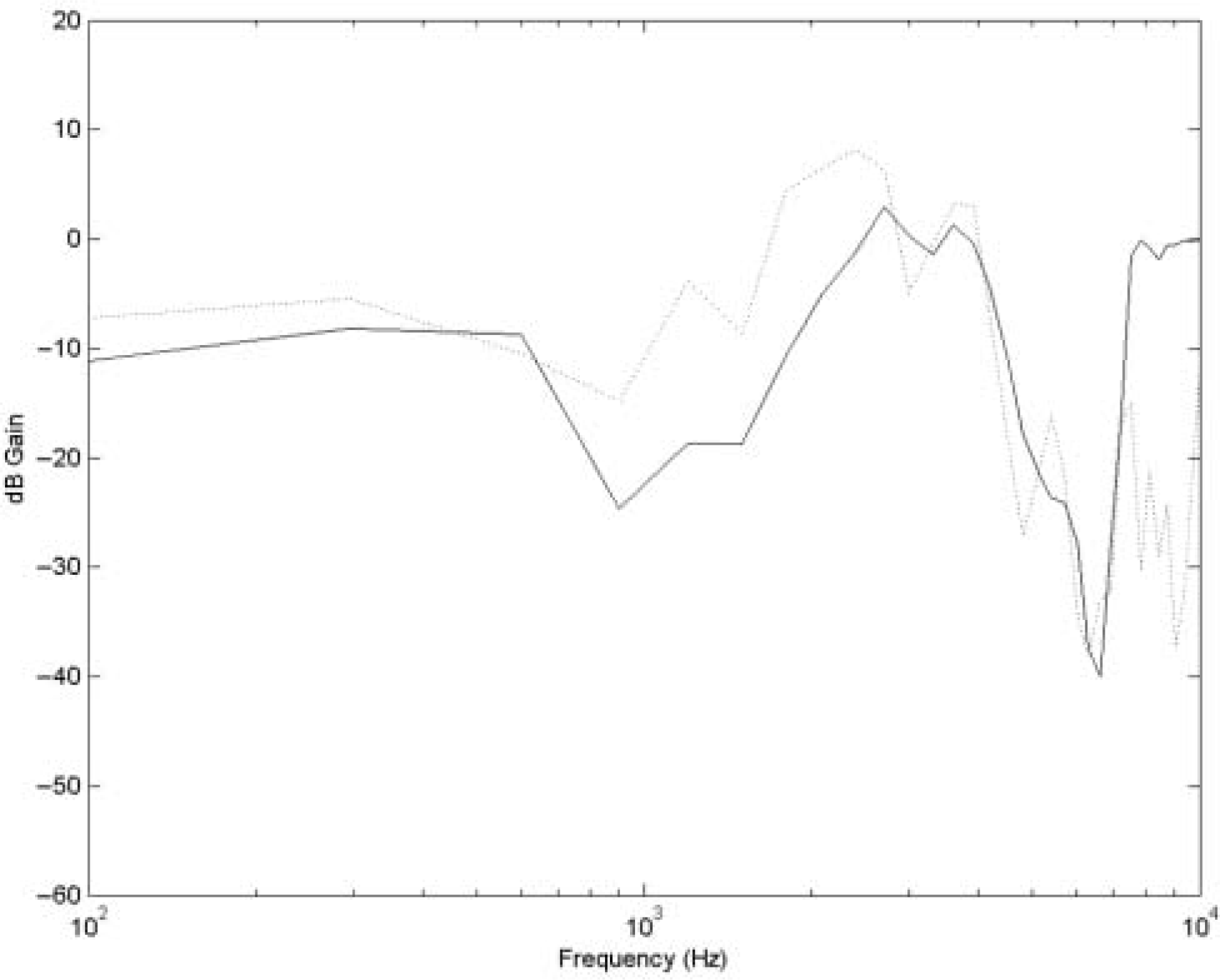
Transfer functions of the open ear canal (solid line) and aided ear (dotted line)
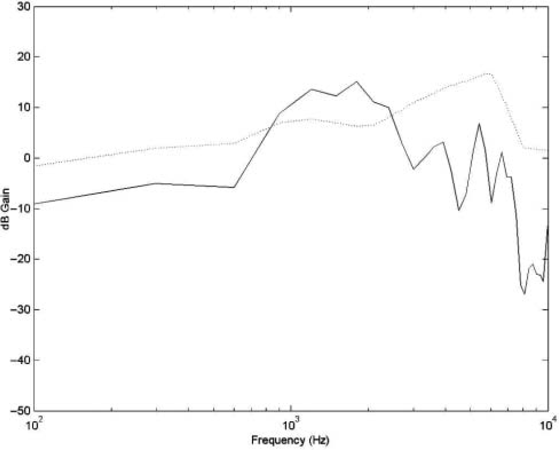
Insertion gain of the aid (solid line) and NAL-NL1 target (dotted line)
It can be seen from Figure 2 that insertion gain of the hearing aid generally did not match the target well. At high and low frequencies the gain was less than the target, and at 1 kHz the gain was slightly above. The mean difference between gain and target from 100 to 8,000 Hz was 10.7 dB. At 1 and 2 kHz the difference between gain and target exceeded 5 dB. At 3, 4, and 6 kHz it exceeded 10 dB. The increase in mismatch with frequency was broadly consistent with the findings of Hawkins and Cook (2003), who compared the manufacturer's predicted gain for different hearing aids with the real-ear insertion gain of 12 patients. They found mismatches between predicted and real-ear gain of −7 dB (range approximately 10 dB) below 2 kHz decreasing to as much as −22 dB (range approximately 20 dB) at 4 kHz (the highest frequency tested). The magnitude of the mismatch between real-ear gain and insertion target shown in Figure 2 appeared to be broadly consistent with the magnitude of mismatch that might be expected in clinics.
Figure 3 shows the difference between the insertion gain of the aid and the NAL-NL1 target. This is the desired gain of the compensation filter. Up to 20 dB gain is required at around 4 to 6 kHz.
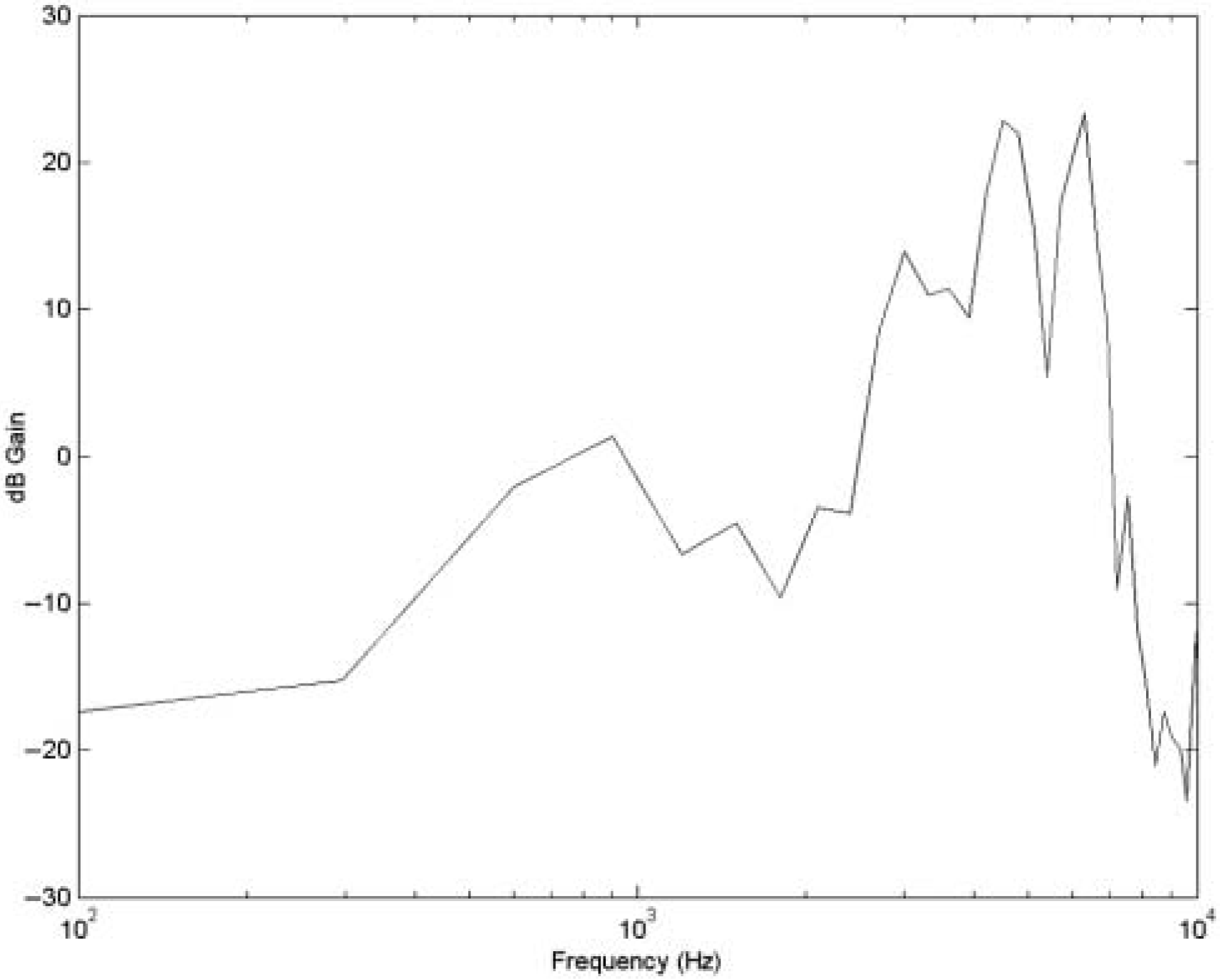
The desired gain of the compensation filter
An FIR filter was then generated to give the desired response using the frequency sampling method. The results using filter order 100 are shown in Figure 4, which shows the impulse response of the filter and the associated gain response. On inspection the filter gain approximates the target gain of Figure 3.
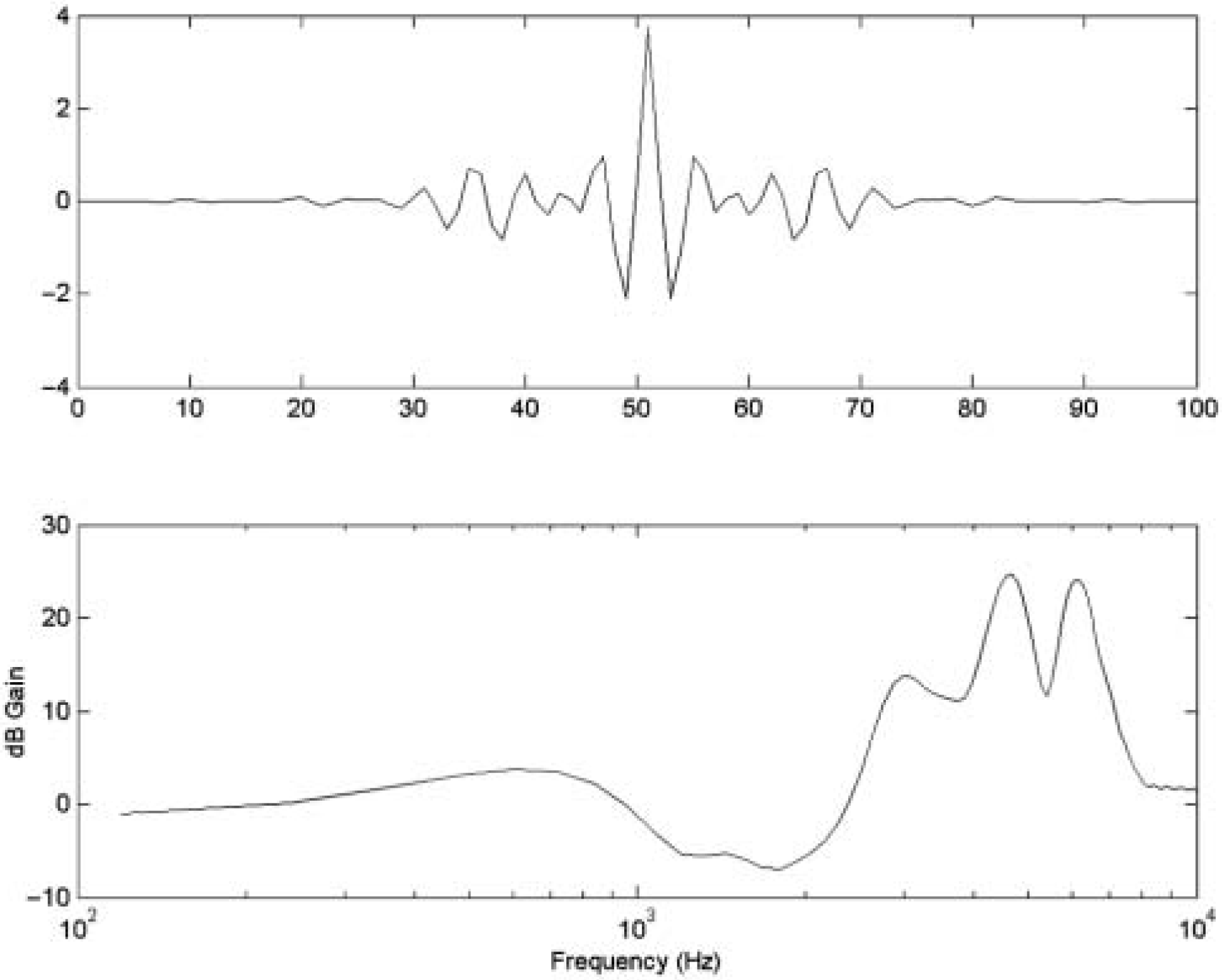
The impulse response and associated gain of the 100-point FIR filter
Finally, the filter was applied to the white noise used to identify the aided response of the system, and a new aided transfer function was measured. This was divided by the response of the open ear measured using the original unfiltered noise to estimate the gain of the hearing aid and filter combined. In practice, the filter could be placed in the processing pathway of a digital aid. Figure 5 compares the gain of the hearing aid and compensation filter to the gain target (65 dB SPL NAL-NL1). The match to targets can be seen to be better at high frequency that that in Figure 2. At the frequencies 0.25, 0.5, 1, 2, 3, 4, and 6 kHz, the gain matched the NAL-NL1 targets within 5 dB, which satisfied the BSA guidelines for performing real-ear measurement (BSA, 2007). Before the filter was applied this was not the case (in Figure 2). The mean difference between gain and target from 100 to 8,000 Hz was now 3.5 dB.

The insertion gain of the combined hearing aid and compensation filter (solid line) and the NAL-NL1 target (dotted line)
Effects of Filter Order on Compensation Error
The effect of the order of the compensation filter on the error between insertion gain and gain targets was explored. The effect of compensation in a real ear was measured with filter orders from 12 to 800. The corresponding group delays of the filters at 24 kHz sampling rate ranged from 0.25 to 16.65 ms.
Table 2 shows the errors between measured insertion gain and gain targets for different orders of filters (mean error between 0.1 and 8 kHz). Table 3 shows the differences between insertion gain and targets at specific audiometric frequencies. It can be seen that the mean error decreases as a function of filter length but that the group delay of the filter increases. A filter length of 100 with an associated group delay of 2.09 ms was required to match the BSA guidelines. With an order 50 (1.04 ms) filter, targets were matched at all frequencies except 1 kHz, where the difference between insertion gain and target was 0.5 dB outside the BSA guidelines at 5.5 dB.
Error Between the Insertion Gain of the Combined Filter and Hearing Aid and the NAL-NL1 Target as a Function of Filter Length and Corresponding Delay

Difference Between the Insertion Gain of the Combined Filter and Hearing Aid and the NAL-NL1 Target at Specific Frequencies
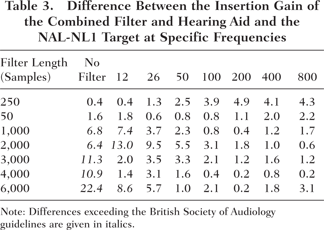
Note: Differences exceeding the British Society of Audiology guidelines are given in italics.
Discussion
The aim of this article was to demonstrate the principle of generating a filter from real-ear measurement that matches the insertion gain in the real ear to target gains from a prescription formula, accounting for the variation in individual ear acoustics. For simplicity, this was limited to the case of a hearing aid set with linear gain. The author did not have the facility to place the filter into the digital pathway of the hearing aid, but for a linear system it does not matter where the filter is placed in the signal pathway (here it was applied to the white noise signal used for system identification).
The process of accounting for the (linear) individual acoustics of the patient's ear is conceptually the first part of real-ear measurement/hearing aid gain adjustment. The next step of verifying appropriate nonlinear gain using different input levels is affected by the first step: The mismatch between the individual ear acoustics and those of an average ear will affect insertion gain measurements at all input levels. Note that the proposed technique does not negate the need to confirm the appropriate compression is applied based on the patient's audiogram, but it should make it easier to match insertion gain to targets for all input levels.
If the filter was applied after the compressor in a nonlinear aid it could still match the gain at the output of the compressor to that desired in the patient's ear (if applied before the compressor it would alter the input level to the compressor and thus the nonlinear gain). An extension of this work would be to use such a filter to compensate for the difference between the response of a hearing aid in a standard coupler (e.g., 2cc or occluded ear simulator) and that in the patient's ear. Coupler measurements could be used to demonstrate that, for a given audiogram and associated nonlinear targets, a hearing aid is able to match targets. A compensation filter generated from REMs could then be used to produce the same gain in an individual's ear.
This article illustrates the principle of the compensation filter. For it to be used in clinics, the software that performs real-ear measurement would need to communicate with the hearing aid programming software (e.g., to calculate the filter required and then program it into the aid). At present, software modules are generally not linked in this way.
The aim of this article was to demonstrate the feasibility of using a filter to compensate for the mismatch between target and real-ear insertion gains, which arises primarily as a consequence of linear individual ear acoustics. As just a demonstration of the principle, the work was limited in scope to the somewhat artificial case of a hearing aid set with linear gain. A useful extension of the work would be to investigate the efficacy of the approach for a range of ears, audiograms, and both linear and nonlinear hearing aids, ideally where the filter is included in the processing pathway of the hearing aid. The approach may need to be modified for open fittings where the forward gain path of the hearing aid interacts with the reverse feedback pathway leaking from the ear canal.
There is an issue of what is an acceptable delay in a hearing aid. Stone and Moore (1999) suggest that a delay of more than 20 ms will cause a disturbing echo between bone and air conducted sound for patients with mild to moderate hearing loss. Very long hearing aid delays can also disrupt speech production and cause problems with speech reading. As shown above, a compensation filter with group delay just over 2 ms was able to match insertion gain to within 5 dB of targets for all frequencies from 250 Hz to 6 kHz. If included in the signal path of an aid, this delay would be additional to the existing digital processing delay of the aid. An important practical consideration if using this technique would be to keep the overall delay within an acceptable range.
There is evidence that having multiple channels in hearing aids, each with potentially different gain and compression settings, can reduce speech intelligibility. Stone and Moore (2008) investigated the effect of increasing the number of compression channels in a vocoder simulation from 1 to 12 on speech intelligibility and found a decrease in intelligibility with the number of channels. Using a broadband filter to compensate for individual ear acoustics as described and then using a small number of channels with adjustable gain and compression may therefore have beneficial effects on speech intelligibility compared to a “graphic equalizer” approach in which gain and compression is adjusted across multiple channels.
It should be noted that while matching the frequency response of a hearing aid to targets is considered an acceptable method of verification and is widely used in clinics, there can be acoustic effects in the time domain that are not obvious in the frequency domain. For example, a sharp resonance in insertion gain may produce associated ringing in the time domain. Before generating a compensation filter it would be best to try and minimize sharp peaks in the frequency domain (and associated effects in the time domain) using ear mold modifications where possible, for example, by adding damping in the mold tubing to make the insertion response less peaked. Where the desired frequency response is achieved, it may still be prudent to check the time domain output of the hearing aid for unwanted signal distortion.
Currently, clinicians spend significant time performing REMs with digital signal processing aids and adjusting hearing aid gains to match targets. The quality of the match depends on the characteristics of the aid and is limited by the number of channels available. The proposed method has potential to improve this matching process.
Glossary
Some nontechnical definitions of terms used in the article are included for the reader's convenience.
Auto spectrum: The auto spectrum of a signal is the Fourier transform (hence spectrum) of the autocorrelation of a signal, also called the power spectrum of the signal. The autocorrelation of the signal gives a measure of the extent to which a signal correlates with a delayed version of itself (correlation is calculated as a function of increasing delay). The autocorrelation of a sine wave is itself a sine wave as with a shift of one period it will perfectly correlate with itself.
Cross-spectrum: The cross-spectrum of two signals is the Fourier transform (hence spectrum) of the cross-correlation function of the two signals. The cross-correlation of two signals gives a measure of the extent to which two signals correlate with each other as a function of the delay (lag) between the two signals. The correlation between the two signals is first calculated with no delay between them, then the delay is gradually increased and the correlation found as a function of the increasing delay.
Dynamic range: The ratio between the largest and smallest values (e.g., sound pressure levels) that a variable can take. In this article, dynamic range refers to values that can be measured. Usually expressed in decibels.
Epoch: Generally means a single time period, but in this article is used to indicate one measurement time window. Several epochs are averaged together to reduce background/measurement noise. In this article one epoch was 33.3 ms.
Fast Fourier transform (FFT): A computationally fast method to calculate the discreet Fourier transform that decomposes a signal into its component frequencies. This is often used in signal analysis to view the component frequencies present in a given signal such as a speech sample.
Finite impulse response (FIR) filter: A type of digital filter. The output of the filter at any point in time is the weighted sum of previous inputs (samples) to the filter. Only a finite number of input samples are weighted to produce the output of the filter, so if the input of the filter drops to zero, the output of the filter will drop to zero after a finite time, hence finite impulse response. FIR filters are inherently stable.
Infinite impulse response (IIR) filter: A type of digital filter. The output of the filter at any point in time is the weighted sum of previous inputs and outputs from the filter. Due to the recursive nature of the filter if the input drops to zero, the output may in theory never reach zero, hence the name infinite impulse response. Such filters may not be stable—an input to the filter may cause the filter output to grow indefinitely.
Frequency sampling: A signal or transfer function viewed in the frequency domain is sampled at a certain frequency spacing (in the same way that sampling in the time domain involves taking samples from a signal with a particular time spacing). A signal that was originally sampled in the time domain will only contain frequencies up to half the sample rate. Hence, if sampling is then done in the frequency domain a fixed number of points will be obtained. In filter design the transfer function of a system such as the ear canal (which is a continuous function) can be frequency sampled. These sampled frequencies can be inverse Fourier transformed to produce the impulse response of an FIR filter that emulates the desired transfer function. Normally windowing is applied to the sampled points before inverse Fourier transformation.
Inverse Fourier transform: Inverts the process of the Fourier transformation, thus transforming a signal viewed in the frequency domain (consisting of individual frequency components each of which has a magnitude and phase) back to the time domain.
Sinc function: A function of the form sin(x)/(x). A symmetrical function that has a large central peak and decays with increasing x. The Fourier transform of a rectangular function (or window) is a sinc function. If a sine wave is multiplied by a rectangular window (a finite time sample is taken) and the Fourier transform is calculated, rather than seeing a sharp peak in the frequency domain, a sinc function is seen with most energy at the sine wave frequency but with additional side bands decaying away.
Spectrum: A spectrum is a frequency domain representation of a signal and often refers to the output of Fourier analysis. The power spectrum shows power as a function of frequency.
Transfer function: A mathematical representation of the relationship between the input and output of a system. Is often viewed in the frequency domain, so at each frequency it would represent the change in magnitude and phase of a signal between the input and output. In this article the input signal is that at the microphone of the hearing aid, and the output signal is that at the probe tube microphone placed near the eardrum.
White noise: A random signal containing equal power at all frequencies.
Windowing: A window function is a function that is zero-valued outside of some chosen interval and has a specific shape inside the window. For instance, a rectangular window is constant inside the interval and zero elsewhere (has the shape of a rectangle), a triangular window has the shape of a triangle inside the interval and is zero elsewhere, and so on. Windowing refers to the process where a signal (data such as frequency sample points) is multiplied by the window function. Windowing is important when signals are Fourier transformed as multiplication in one domain (in the example of frequency sampling above, windowing is applied in the frequency domain) will be equivalent to convolution after Fourier transformation (e.g., in the time domain) and no widowing is equivalent to applying a rectangular filter covering the full range of frequencies up to half the sampling rate. The effect of the window function will be to change the shape of the Fourier transformed signal. In this article different windows were applied to the frequency samples taken from the transfer function of the hearing aid/ear canal system before the values were inverse Fourier transformed to produce an FIR filter. The window function known as the “Barlett” window was found to produce the best overall match across frequencies between real-ear insertion gain and prescription targets.
Footnotes
1.
Basic definitions of terms are given in the glossary.