Evaluation of a decomposition-based interpolation method for fourth-order fiber-orientation tensors: An eigensystem approach

Abstract

We propose and assess a new decomposition-based interpolation method on fourth-order fiber-orientation tensors. This method can be used to change the resolution of discretized fields of fiber-orientation tensors, e.g., obtained from flow simulations or computer tomography, which are common in the context of short- and long-fiber–reinforced composites. The proposed interpolation method separates information on structure and orientation using a parametrization which is based on tensor components and a unique eigensystem. To identify this unique eigensystem of a given fourth-order fiber-orientation tensor in the absence of material symmetry, we propose a sign convention on tensor coefficients. We explicitly discuss challenges associated with material symmetries, e.g., non-distinct eigenvalues of the second-order fiber-orientation tensor and propose algorithms to obtain a unique set of parameters combined with a minimal number of eigensystems of a given fourth-order fiber-orientation tensor. As a side product, we specify for the first time, parametrizations and admissible parameter ranges of cubic, tetragonal, and trigonal fiber-orientation tensors. Visualizations in terms of truncated Fourier series, quartic plots, and tensor glyphs are compared.

1. Introduction

1.1. State of the art

The development and design process of discontinuous fiber-reinforced composites [1] is nowadays supported by so-called virtual process chains [2, 3]. A virtual process chain usually includes the simulation of the mold-filling process [4–6] and subsequent structural–mechanical investigation of the component performance, taking into account the local microstructure [7–10]. The microstructure evolves during the form-filling flow and the resulting local orientation of fibers largely determines the local mechanical properties. A complete descriptor of the local fiber-orientation within a specified reference volume in terms of one-point statistics [11] is the fiber-orientation distribution function, which unfortunately is mostly unknown. However, averages of the local distribution function in terms of fiber-orientation tensors [4, 12] can be obtained both from simulations and experimentally. A spatial distribution, i.e., a field, of such fiber-orientation tensors is required to assess the mechanical performance of a composite part within a structural analysis. Techniques to perform such structural analysis range from, e.g., approaches based on mixture theory [13, 14], asymptotic homogenization [15, 16], and finite element method [17] to artificial neural networks [18, 19]. All approaches require a suitable resolution of the local microstructure descriptor. As fiber-orientation tensors act as state variables within most flow simulations [5, 20–22], fields of these tensors naturally occur within virtual process chains. Alternatively, fields of fiber-orientation tensors can be identified experimentally by computer tomography (CT) analysis [23–28]. Regardless of how a field of fiber-orientation tensors has been determined, there is usually a need to perform a mapping [29–31] from the discretization, the tensors have been obtained on, to a discretization which is appropriate for the structural simulation. Interpolation methods for fiber-orientation tensors can be adapted from a related field in medicine. In medicine, magnetic resonance imaging (MRI) is used to identify three-dimensional gray value images of tissues. Diffusion-weighted magnetic resonance imaging (DW-MRI) combines multiple MRI sequences to measure the diffusion of water molecules within tissues, thereby obtaining structural information on the tissue. The measured information is encoded by a three-dimensional field of diffusion tensors [32, 33]. As diffusion tensors differ from second-order fiber-orientation tensors only by a missing constraint on the trace, algorithms developed in medicine for interpolation of three-dimensional fields of diffusion tensors can be adopted to fiber-orientation tensors [29]. A selection of interpolation methods on DW-MRI diffusion tensors is given by early works [34–36] as well as a small selection of references [37–45] indicating the relevance of this field. The aforementioned contributions are accompanied by application-driven works [46, 47] or methods focusing on the underlying partial differential equations [48]. However, most of the methods are limited to second-order tensors and only a few deal with fourth-order tensors [49–51].

In the field of structural mechanics, on the contrary, fourth-order fiber-orientation tensors are increasingly used [52]. Insights into the algebra of fourth-order fiber-orientation tensors [53, 54] allow for the attempt to transfer interpolation methods designed for diffusion tensors to fourth-order fiber-orientation tensors. Bauer and Böhlke [55] combine a parametrization of fourth-order fiber-orientation tensors with algebraic constraints to derive admissible parameter ranges which represent the variety of the fiber-orientation tensor for selected material symmetries. The utilized parametrization is based on an a priori selected coordinate system, acting as eigensystem of both the second- and fourth-order parts of the fiber-orientation tensor of interest. The multiplicity of eigensystems of second-order diffusion and fiber-orientation tensors and uniqueness of projector representations are discussed, e.g., by Kraußand Kärger [29], Basser and Pajevic [56], and Hasan et al. [57].

1.2. Notation

Symbolic tensor notation is preferred in this paper. Tensors of first order are denoted by bold lowercase letters such as $\mathbf{q}$ , $\mathbf{n}$ , $\mathbf{v}$ , and $\mathbf{e}$ . Tensors of second order are denoted by bold uppercase letters like $\mathbf{N}$ or $\mathbf{Q}$ and fourth-order tensors are denoted by, e.g., $\mathbb{N}$ or $\mathbb{D}$ . Tensorial quantities are defined in a three-dimensional space, unless otherwise stated. A linear mapping of a second-order by a fourth-order tensor reads as $\mathbf{A}=\mathbb{C}\left[\mathbf{B}\right]$ . The scalar product between two tensors of arbitrary order is denoted by · which, e.g., reads as $\mathbf{A}·\mathbf{B}$ . The $k\mathrm{th}$ dyadic product of, e.g., a first-order tensor $\mathbf{a}$ is denoted by ${\mathbf{a}}^{\otimes k}$ yielding, e.g., ${\mathbf{a}}^{\otimes 3}=\mathbf{a}\otimes \mathbf{a}\otimes \mathbf{a}$ . An orthonormal basis is denoted by $\left\{{\mathbf{e}}_i\right\}$ with ${\mathbf{e}}_i·{\mathbf{e}}_j={\delta }_{\mathrm{ij}}$ and the Kronecker delta ${\delta }_{\mathrm{ij}}$ . If a matrix of tensor components is used in mixed notation, the coefficient matrix is directly followed by the tensor basis where the first index of the basis corresponds to the rows of the components matrix and the second one to the columns. Summation convention applies, unless otherwise stated. Representations in index notation always refer to an orthonormal basis. The Rayleigh product is used to represent an active rotation of a physical quantity and for a first-order tensor is defined by $\mathbf{Q}★\mathbf{n}=n_i\mathbf{Q}{\mathbf{e}}_i$ . Sets, i.e., collections of quantities, are denoted by calligraphic symbols, e.g., $\mathcal{F}$ and are constructed by curly braces. Inside the curly braces, elements of the set are given explicitly, or by a generator expression following the pattern $\left\{\mathrm{quantity}|\mathrm{condition}\mathrm{fulfilled}\mathrm{by}\mathrm{elements}\mathrm{contained}\mathrm{in}\mathrm{set}\right\}$ . We use standard notation to represent the binomial coefficients, i.e., $\left(\begin{array}{c}2k\hfill \\ \multicolumn{1}{c}{k}\end{array}\right)$ . Although this work and related code is based on [58, 59], numbering and indices follow the continuum mechanics convention starting at one.

1.3. Contribution

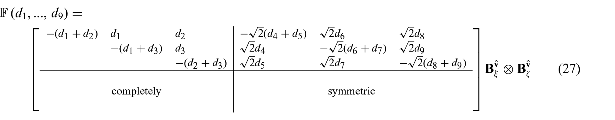
For a given discretized spatial field of fourth-order fiber-orientation tensors, we are interested in heuristic algorithms which interpolate the given field, generating a field of interpolated fourth-order fiber-orientation tensors. The distances of the spatial point of interest to its nearest neighbors might be interpreted as weights. Within this work, we evaluate a new decomposition-based interpolation method for fiber-orientation tensors of fourth order. The new method is based on the parametrization of Bauer and Böhlke [55]. This parametrization represents a fourth-order fiber-orientation tensor in terms of tensor components within an eigensystem of the tensor itself, therefore naturally separating structural and orientational information. The proposed interpolation method is a weighted average of the tensor components within their respective eigensystems. Therefore, the structural properties are encoded in terms of tensor components and the orientational information is encoded in terms of the respective eigensystems. In consequence, the identification of an eigensystem for each individual tensor involved in the interpolation is required. However, the parametrization of [55] is developed to generate fiber-orientation tensors based on a given eigensystem combined with given structural parameters. If in contrast, a given tensor is to be analyzed based on the parametrization, the first step is to determine the eigensystem of the tensor. This determination showed to be a non-trivial task, if the tensor being analyzed has at least partial material symmetry, either within its second- or fourth-order parts. Therefore, as a by-product, we investigate edge cases, caused by (partial) material symmetry, of fourth-order fiber-orientation tensors, extending the work of Bauer and Böhlke [55]. In particular, we study subspaces of fourth-order fiber-orientation tensors induced by cubic, tetragonal, and trigonal material symmetry. As a result, representations of fourth-order cubic, tetragonal, and trigonal fiber-orientation tensors are presented in terms of the aforementioned parametrization, each supplemented by admissible parameter ranges. Since the new interpolation method is built on a parametrization that naturally includes material symmetries, the interpolation method preserves any existing material symmetry of the tensors to be interpolated.

This paper is organized as follows. A brief definition of fiber-orientation tensors in section 1.4 is followed by a classification of problems in section 2. We distinguish three problems which we call averaging, disassembly, and interpolation problem and within this work focus on the latter. In section 3.1, we briefly discuss different classes of interpolation methods. We focus on decomposition-based methods as well as the interpolation of second-order tensors. We explicitly discuss the inherent ambiguity of eigensystems of second-order tensors and the association with the elements of the orthotropic symmetry group (see section 3.2.1). We recite an adoption of the Karcher mean in section 3.2.2. With a note on frequently used structural descriptors of second-order fiber-orientation tensors in section 3.2.3, we close the discussion of second-order information and focus on fourth-order fiber-orientation tensors in section 4. After a recap of the eigensystem-based parametrization of fourth-order fiber-orientation tensors [55] in section 4.1, we outline the new interpolation method in section 4.2. In section 4.3, we introduce a new convention to obtain a unique eigensystem of any triclinic fourth-order fiber-orientation tensor. Within section 4.4, we discuss limitations of this convention-based procedure in the presence of material symmetry. For each edge case, we demonstrate the identification of possible multiple eigensystems combined with a unique set of structural parameters. We apply the new method on examples in section 5. Parametrizations and admissible parameter ranges of cubic, tetragonal, and trigonal fourth-order fiber-orientation tensors are given in Appendices 1–3, respectively. Eigenvalues and eigentensors of irreducible fourth-order tensors of transversely isotropic, trigonal, tetragonal, and orthotropic symmetry are presented in Appendix 4. We close this paper with a discussion and comparison of visualization methods for fourth-order fiber-orientation tensors, focusing on truncated Fourier series, quartic plots, and glyph representations.

1.4. Fiber-orientation tensors

The fiber-orientation distribution function (FODF)

$$\psi :{\mathcal{S}}^2\to \mathbb{R},\mathrm{with}{\mathcal{S}}^2=\{\mathbf{n}\in {\mathbb{R}}^3|\Vert \mathbf{n}\Vert =1\}$$

(1)

maps any direction $\mathbf{n}$ , i.e., any point on the unit sphere in three dimensions ${\mathcal{S}}^2$ , onto a scalar value $\psi \left(\mathbf{n}\right)$ and is an exact descriptor of the one-point statistics of the orientation of fibers in a given reference volume. With ‖·‖ denoting the standard Euclidian metric. The fiber-orientation distribution function $\psi \left(\mathbf{n}\right)$ is non-negative $\psi \ge 0$ , normalized ${\int }_{{\mathcal{S}}^2}\psi \left(\mathbf{n}\right)\mathrm{d}n=1$ and symmetric $\psi (-\mathbf{n})=\psi \left(\mathbf{n}\right)$ [4, 12, 55] and integration over a specific surface element $\mathcal{A}\subset {\mathcal{S}}^2$ , i.e.,

$$p_{\mathcal{A}}={\int }_{\mathcal{A}}\psi \left(\mathbf{n}\right)\mathrm{d}n$$

(2)

quantifies the fraction $p_{\mathcal{A}}$ of fibers pointing into directions contained in $\mathcal{A}$ . The fiber-orientation distribution function $\psi \left(\mathbf{n}\right)$ may be expressed as a three-dimensional tensorial Fourier series in terms of fiber-orientation tensors of $k\mathrm{th}$ order ${\mathbb{N}}_{<k>}$

$$\psi \left(\mathbf{n}\right)=\frac{1}{4\pi }\sum _{k=0}^{\infty }\frac{2k+1}{2^k}\left(\begin{array}{c}2k\hfill \\ \multicolumn{1}{c}{k}\end{array}\right)\mathrm{dev}\left({\mathbb{N}}_{〈k〉}\right)·{\mathbf{n}}^{\otimes k}$$

(3)

called spherical harmonic expansion [12, page 154]. The operator $\mathrm{dev}(·)$ extracts the deviatoric part and its definition for higher-order tensors is given in Spencer [60]. In most engineering applications, the fiber-orientation distribution function is unknown and second- and fourth-order averages of this function represent a sufficient amount of information on the fibers’ orientation. The second- and fourth-order averages of the fiber-orientation distribution function are given by fiber-orientation tensors of Kanatani [12] first kind of second and fourth order, depicted by $\mathbf{N}$ and $\mathbb{N}$ , respectively. These tensors are defined by weighted integration of moment tensors, i.e.,

$$\mathbf{N}={\int }_{{\mathcal{S}}^2}\psi \left(\mathbf{n}\right)\mathbf{n}\otimes \mathbf{n}\mathrm{d}n,$$

(4)

$$\mathbb{N}={\int }_{{\mathcal{S}}^2}\psi \left(\mathbf{n}\right)\mathbf{n}\otimes \mathbf{n}\otimes \mathbf{n}\otimes \mathbf{n}\mathrm{d}n$$

(5)

with the weights being defined by the fiber-orientation distribution function $\psi (\mathbf{n})$ . Fiber-orientation tensors are completely symmetric, i.e., have any index symmetry and are positive semi-definite in the sense of both

$$\mathbb{N}·(\mathbf{q}\otimes \mathbf{q}\otimes \mathbf{q}\otimes \mathbf{q})\ge 0\forall \mathbf{q}\in {\mathbb{R}}^d$$

(6)

and

$$\mathbf{S}·\mathbb{N}\left[\mathbf{S}\right]\ge 0\forall \mathbf{S}\in \mathrm{Sy}{\mathrm{m}}_2(d)$$

(7)

for dimensions two and three, i.e., $d=2$ or $d=3$ , with the space of symmetric second-order tensors $\mathrm{Sy}{\mathrm{m}}_2(d)$ , the $d$ -dimensional vector space ${\mathbb{R}}^d$ , and the dyadic product between two tensors $\mathbf{a}$ and $\mathbf{b}$ denoted by $\mathbf{a}\otimes \mathbf{b}$ . A detailed discussion is given by Bauer et al. [54]. It is worth noting that any fourth-order fiber-orientation tensor contains a second-order fiber-orientation tensor such that

$$\mathbf{N}=\mathbb{N}\left[\mathbf{I}\right]$$

(8)

holds with the identity on second-order tensors $\mathbf{I}={\delta }_{\mathrm{ij}}{\mathbf{e}}_i\otimes {\mathbf{e}}_j$ . The trace of $\mathbf{N}$ is normalized, i.e.,

$$\mathrm{tr}\left(\mathbf{N}\right)=\mathbf{N}·\mathbf{I}=1$$

(9)

holds.

2. Averaging, disassembly, and interpolation

2.1. Motivation

Since the local mechanical properties of a discontinuous fiber-reinforced composite depend on the local orientation of the fibers, the quantification of this local fiber-orientation is an essential part of the computer-aided design process of such materials. Suppose, for a component geometry under investigation, the local fiber-orientation is given in the form of a spatially discretized field of fourth-order fiber-orientation tensors. This field is therefore based on a spatial discretization, i.e., each individual fiber-orientation tensor within this discrete field is assigned to a reference volume of the component and describes the average fiber-orientation within this reference volume. For simplification, let us also assume that the component geometry to be investigated is planar and the discretization is chosen in such a way that the individual reference volumes do not overlap. A small section with only four reference volumes of such a two-dimensional discretization is shown as an example in Figure 1(a).

Figure 1.

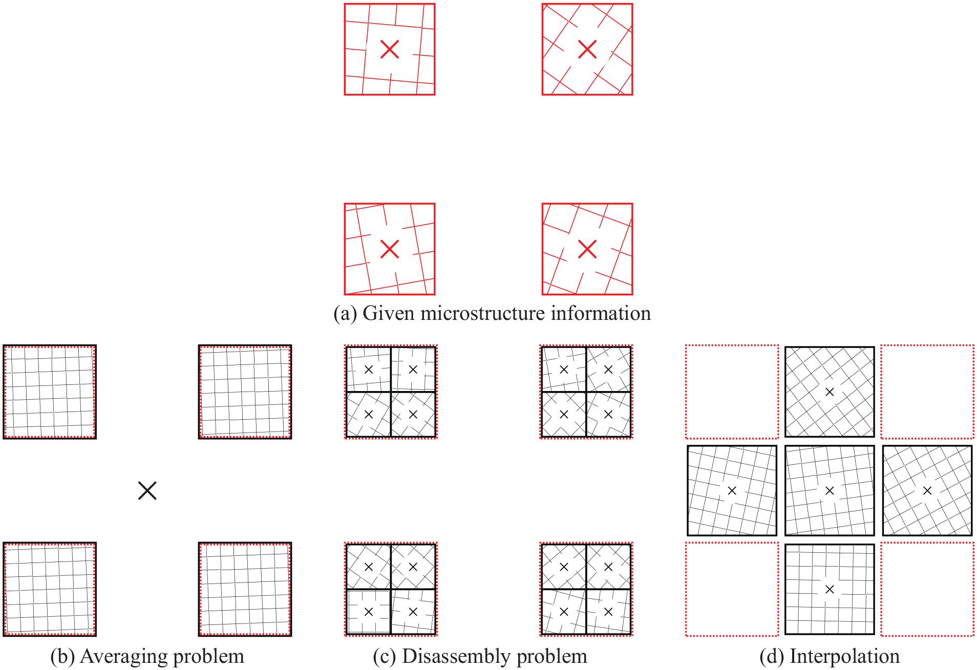
Schematic example of a given discretization of microstructure information. The example discretization is flat and consists of four non-overlapping reference volumes of equal size (a). The averaging, disassembly, and interpolation problems are depicted in (b), (c), and (d), respectively. The measured grid data are depicted in red, whereas the target volumes are colored in black. Most discretizations associate each information, e.g., a specific microstructure descriptor, with a spatial point, i.e., a location. We indicate the associated locations of the measured data and the target volumes with red and black crosses, respectively.

If for the considered component, engineering tasks are to be solved, the spatial discretization of the available fiber-orientation field is often not optimal for the subsequent analysis steps and a change of the spatial discretization is necessary. We categorize such changes of the spatial discretization into three different problems—averaging, disassembly, and interpolation. Averaging corresponds to combining reference volumes, whereas disassembly can be interpreted as splitting up a given reference volume and interpolation can be seen as a refinement of the given spatial field, usually incorporating some kind of weights or distance measure. The weights for the interpolation might be given, e.g., based on the spatial distance between reference volumes which are to be combined. Brannon [61] discusses the problem of interpolating or averaging physical quantities which are related to directions and rotations, demonstrating that the interpolation or averaging methods might be evaluated with respect to specific problems rather than in a general way. We analyze each of the three problems and discuss existing solutions to the interpolation problem before insights based on irreducible tensors and material symmetry lead to a new interpolation method for fourth-order fiber-orientation tensors.

2.2. The averaging problem

In a given field of microstructure descriptors, e.g., fiber-orientation tensors, each single entity is associated with a reference volume, which microstructure it describes. If the reference volume is considered a thermodynamic system, microstructure descriptors may be interpreted as intensive state variables, which are additive in a weighted sense. That is, the state variable of the union of two subsystems is the volume-weighted sum of the respective state variables of the subsystems. In the field of micromechanics, this property is usually represented by the exact split of the volume average over a system into the weighted sums of volume averages over the subsystems. In consequence, the fiber-orientation distribution function associated with a reference volume ${\mathcal{V}}_{\mathrm{total}}={\mathcal{V}}_1\cup {\mathcal{V}}_2$ consisting of two reference volumes ${\mathcal{V}}_1$ and ${\mathcal{V}}_2$ depicted in Figure 2, is given by

$${\psi }_{\mathrm{total}}=\frac{1}{\left|{\mathcal{V}}_{\mathrm{total}}\right|}(\left|{\mathcal{V}}_1\right|{\psi }_1+\left|{\mathcal{V}}_2\right|{\psi }_2)$$

(10)

where ${\psi }_i$ is associated with ${\mathcal{V}}_i$ for $i\in \{1,2\}$ , see the works Krauß et al. [31] and Krauß and Kärger [29]. The same holds for fiber-orientation tensors of any order, e.g., depicted exemplarily as fourth-order fiber-orientation tensors by

$${\mathbb{N}}_{\mathrm{total}}=\frac{1}{\left|{\mathcal{V}}_{\mathrm{total}}\right|}(\left|{\mathcal{V}}_1\right|{\mathbb{N}}_1+\left|{\mathcal{V}}_2\right|{\mathbb{N}}_2)$$

(11)

with ${\mathbb{N}}_i$ associated with ${\mathcal{V}}_i$ for $i\in \{1,2,\mathrm{total}\}$ .

Figure 2.

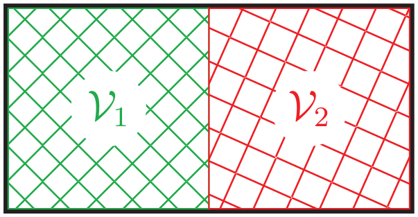
Minimal example of the averaging problem with two reference volumes with equal size, arranged next to each other.

In consequence, the unique solution of the averaging problem of fiber-orientation tensors is known directly and given by the arithmetic mean of tensor components in an arbitrary, but homogeneous, coordinate system. Interpolation methods which take the arithmetic mean of tensors have an averaging character.

2.3. The disassembly problem

We define the disassembly problem as the reversal of the averaging problem. In consequence, the disassembly problem is the identification of fiber-orientation tensors ${\mathbb{N}}_i$ for a given set of reference volumes ${\mathcal{V}}_i$ with $i\in \{1,...,n\}$ and fixed number $n$ which fulfill the equation

$${\mathbb{N}}_{\mathrm{total}}=\frac{1}{\left|{\mathcal{V}}_{\mathrm{total}}\right|}\sum _{i=1}^n\left|{\mathcal{V}}_i\right|{\mathbb{N}}_i$$

(12)

with the reference volume ${\mathcal{V}}_{\mathrm{total}}={\cup }_{i=1}^n{\mathcal{V}}_i$ and quantity ${\mathbb{N}}_i$ associated with reference volume ${\mathcal{V}}_i$ for $i\in \{1,..,n,\mathrm{total}\}$ . The disassembly problem always has the trivial solution

$${\mathbb{N}}_i={\mathbb{N}}_{\mathrm{total}}\forall i\in \{1,...,n\}.$$

(13)

If ${\mathbb{N}}_{\mathrm{total}}$ corresponds to the unidirectional fiber-orientation state, the trivial solution given in equation (13) is the only solution. In general, however, the disassembly problem is ill-posed and solutions are not necessarily unique. For a variable number of individual volumes $n$ , every ${\mathbb{N}}_{\mathrm{total}}$ can be represented by sufficiently many differently oriented unidirectional states [54, 62]. If these unidirectional states are optimally weighted, not more than 15 are necessary [54] in three-dimensional problems. Schemmann et al. [63] fit an empirical fiber-orientation distribution, consisting of Dirac distributions, to a given fiber-orientation tensor. The disassembly problem is related to the problem of approximating a fiber-orientation distribution function by given tensors [52, 64] but adds a spatial aspect in terms of reference volumes.

2.4. The interpolation problem

The required spatial resolution of fields of fiber-orientation tensors differs between individual steps of a virtual process chain. Solving initial boundary value problems on microstructured materials may require high-resolution fields of microstructural information, depending on the effects being studied and the scales associated with those effects. Obtaining such high-resolution fields of microstructure information often represents a bottleneck in the virtual process chain. One example is the determination of local fiber-orientation tensors using CT on long-fiber-reinforced composites such as sheet molding compound (SMC) and long-fiber–reinforced thermoplastics (LFT). The geometric dimensions of fibers in fiber-reinforced composites define the necessary resolution of CT scans. The smaller the diameter of the fibers, the higher the resolution of the CT scan must be selected [30]. The fiber diameter defines requirements on the CT resolution, which is independent of the desired spatial resolution of the tensor field.

If microstructure information on a coarse macroscopic grid is of interest, the CT scans may be restricted to a sparse grid of scanned reference volumes on the component. In a next step, the exact solution of the averaging problem discussed in section 2.2 can be used to average the sparse grid data of the scanned fiber-orientation tensors to values associated with the nodes of the coarse macroscopic grid [30]. The volumetric sizes of the staggered grid of scanned regions have to be carefully selected in order to reflect the microstructure of interest.

If, on the contrary, a granular field of local microstructure information is of interest, an identical scanning setup on a staggered grid of small reference volumes can be used with a successive refinement by interpolation. However, the evolution of fiber states between the measured points of the staggered CT grid is defined by a physical process, which itself is described by partial differential equations and the initial and boundary conditions during the manufacturing process of the component at hand. Therefore, simulation of such a physical process is impractical, although desirable. In consequence, interpolation methods are necessary to refine a given grid of measured orientation states. This refinement is called the interpolation problem.

Both the disassembly problem and the interpolation problem aim at a refinement of grid data. However, the reference volumes associated with the refined grid of the disassembly problem are contained completely within the measured reference volumes of the coarse grid. In contrast, interpolated orientation states can be associated with reference volumes which are located between measured reference volumes. This is visualized schematically in Figure 1(d). In general, the reference volumes might overlap.

An interpolation problem is specified by data on a source discretization and a specific target discretization onto which the date is to be interpolated. A solution to an interpolation problem depends on the type of weighting as well as the selected interpolation method. In this work, local weights, which depend on the meshing algorithm, the finite element type, and the shape functions, are preferred over global weights, such as Shepard’s method [30]. Weights on these two-dimensional fields are obtained by triangulation with linear shape functions.

3. Interpolation of second-order fiber-orientation tensors

3.1. Classes of interpolation methods

Interpolation methods for fiber-orientation tensors can be adapted from a related field in medicine. In medicine, MRI is used to identify three-dimensional gray value images of tissues. DW-MRI combines multiple MRI sequences to measure the diffusion of water molecules within tissues, thereby obtaining structural information on the tissue. The measured information is encoded by a three-dimensional field of diffusion tensors [32,33]. The diffusion tensors determined by DW-MRI are positive semi-definite and symmetric tensors of second order. Second-order fiber-orientation tensors can thus be identified as dimensionless diffusion tensors with fixed trace, see equation (9). In consequence, algorithms developed in medicine for interpolation of three-dimensional fields of diffusion tensors can be adopted to fiber-orientation tensors.

The exact solution to the averaging problem (section 2.2), hereafter called component averaging, maybe applied as an interpolation method by component-wise interpolation of tensor components in an arbitrary reference coordinate system. However, interpolation by component averaging leads to the swelling effect [37, 39, 41, 42], i.e., a tendency towards isotropic states, and does not reflect expectations on flow fields of fiber-orientation tensors. Association of component averaging with the averaging problem, see section 2.2 explains the swelling effect. Interpolation methods other than component averaging can be categorized into two groups—Riemannian interpolation methods and decomposition-based interpolation methods. Riemannian methods on diffusion tensors [37–39, 65] treat tensors as elements on a Riemannian symmetric space and use metrics on this manifold. As the new interpolation method proposed in section 4 belongs to the decomposition methods, we focus on this class of methods.

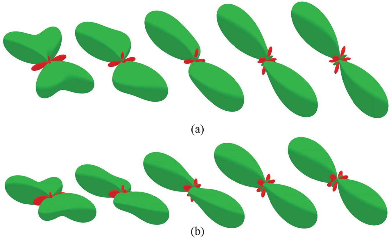
A first intuition on the differences between component averaging and decomposition-based methods is given by Figure 3, in which two elongated fiber-orientation tensors differing by almost a quarter rotation around one axis perpendicular to the large eigenvector are interpolated using two interpolation methods. Columns two, three, and four represent interpolated fiber-orientation tensors obtained by two different interpolation methods. The interpolated states in the upper row are calculated by averaging tensor components in a global reference coordinate system, i.e., the exact solution of an averaging problem with varying volume fractions. The lower row shows the new interpolation method and indicates its decomposition-based character, as the interpolated states preserve the homogeneous structure of the left- and right-most orientation states. As this method is a decomposition method and the reference fiber-orientation tensors are both unidirectional, the interpolated tensors only differ by a rotation. Associating this interpolation problem with a flow field and a single fiber, would clearly indicate high suitability of the decomposition method. However, as the interpolated fiber-orientation tensors describe averages of associated volumes instead of single fibers, judgment on the suitability of the different methods is difficult. If the angle between the given fiber-orientation tensors in Figure 3 is exactly ninety degrees, the solution of the decomposition-based method is not unique.

Figure 3.

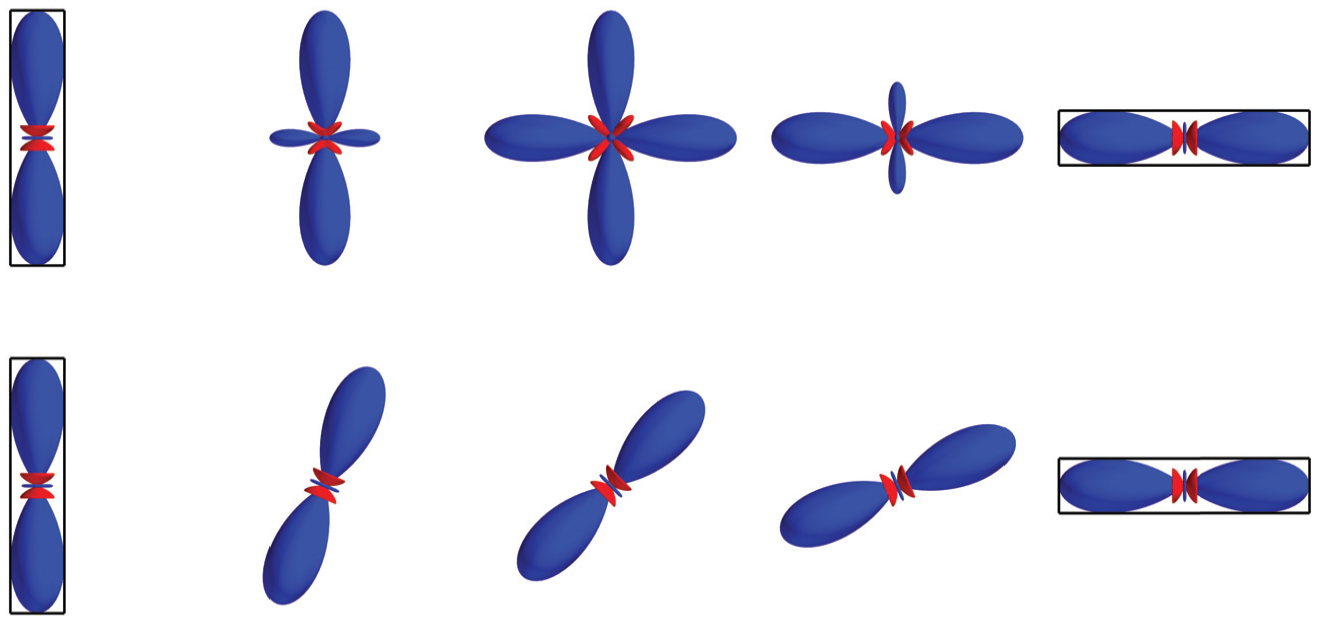
Two unidirectional fiber-orientation tensors of fourth order, which differ by a bit less than a quarter rotation, are visualized in the outer columns and represent an interpolation problem. The three-dimensional plots show reconstructed fiber-orientation distribution functions obtained by truncated Fourier series expansion in fiber-orientation tensors up to fourth-order, see [64, equation 31]. Positive parts of the distribution functions are colored blue, whereas negative parts are color-coded red, following [64] and a detailed discussion on visualization in Appendix 5. This figure follows [37, Figure 3].

Decomposition-based interpolation methods [41, 47, 50] decompose tensors into information on the orientation and structure. The information on the orientation can, e.g., be encoded as a coordinate system spanned by eigenvectors of the diffusion or fiber-orientation tensor and might also be referred to as rotation [66]. The structural information is also referred to as shape [47, 50], type of material symmetry [67], or scaling [66] and is commonly encoded by invariants. The independent interpolation of structure and orientation implies that interpolations of two tensors, which differ only by their orientation, have constant structure, i.e., the interpolation preserves the structure. An example of such a structure-preserving decomposition-based interpolation is given in the lower row in Figure 3. Likewise, decomposition-based interpolations between two non-identical tensors sharing identical orientations differ only by their structure. A decomposition-based interpolation of two fourth-order tensors which differ only by structure is given in Figure 8.

3.2. Decomposition-based methods

3.2.1. Orientation and multiplicity of eigensystems

Decomposition of a second-order fiber-orientation tensor $\mathbf{N}$ into a rotation and eigenvalues, encoding its structural information, is briefly summarized following [55], emphasizing the non-uniqueness of the eigensystem. As $\mathbf{N}$ is symmetric and positive semi-definite, it can be diagonalized, i.e., pairs of eigenvalues ${\lambda }_i$ with ${\lambda }_i\ge 0$ and orthonormal eigenvectors ${\hat{\mathbf{v}}}_i$ of arbitrary sign for $i\in \{1,2,3\}$ exist, such that

$$\mathbf{N}=N_{\mathrm{ij}}^{(2)}{\mathbf{e}}_i\otimes {\mathbf{e}}_j=\sum _{i=1}^3{\lambda }_i{\hat{\mathbf{v}}}_i\otimes {\hat{\mathbf{v}}}_i=\left[\begin{array}{ccc}{\lambda }_1\hfill & 0\hfill & 0\hfill \\ \multicolumn{1}{c}{}& {\lambda }_2\hfill & 0\hfill \\ \multicolumn{1}{c}{\mathrm{sym}}& \hfill & {\lambda }_3\hfill \end{array}\right]{\hat{\mathbf{v}}}_i\otimes {\hat{\mathbf{v}}}_j$$

(14)

holds. If the vector ${\hat{\mathbf{v}}}_i$ is eigenvector of $\mathbf{N}$ , so is the vector $-{\hat{\mathbf{v}}}_i$ . In consequence, any combination of signs of the eigenvectors representing a orthonormal triplet of right-handed vectors, i.e.,

$${\left\{{\mathbf{v}}_i\right\}}_1=\{{\hat{\mathbf{v}}}_1,{\hat{\mathbf{v}}}_2,{\hat{\mathbf{v}}}_1\times {\hat{\mathbf{v}}}_2\},$$

(15)

$${\left\{{\mathbf{v}}_i\right\}}_2=\{{\hat{\mathbf{v}}}_1,-{\hat{\mathbf{v}}}_2,{\hat{\mathbf{v}}}_1\times -{\hat{\mathbf{v}}}_2\},$$

(16)

$${\left\{{\mathbf{v}}_i\right\}}_3=\{-{\hat{\mathbf{v}}}_1,{\hat{\mathbf{v}}}_2,-{\hat{\mathbf{v}}}_1\times {\hat{\mathbf{v}}}_2\},$$

(17)

$${\left\{{\mathbf{v}}_i\right\}}_4=\{-{\hat{\mathbf{v}}}_1,-{\hat{\mathbf{v}}}_2,-{\hat{\mathbf{v}}}_1\times -{\hat{\mathbf{v}}}_2\}$$

(18)

is a valid eigensystem of $\mathbf{N}$ and corresponds to a unique rotation, which is defined by an orthogonal tensor

$${\mathbf{Q}}_j={\mathbf{v}}_i\otimes {\mathbf{e}}_i\mathrm{with}{\mathbf{v}}_i\mathrm{in}{\left\{{\mathbf{v}}_i\right\}}_j\forall j\in \{1,2,3,4\},$$

(19)

mapping the arbitrary but fixed basis $\left\{{\mathbf{e}}_i\right\}$ onto the basis ${\left\{{\mathbf{v}}_i\right\}}_j$ [42, 57, 68]. In consequence, second-order fiber-orientation tensors with distinct eigenvalues do not define one coordinate system uniquely but define four eigensystems which differ by signs of their base vectors. The directional information which is contained in $\mathbf{N}$ does not include information, which could be used to motivate the selection of one out of the four eigensystems. This observation follows from the material symmetries of second-order tensors. The weakest material symmetry [67, 69, 70] of symmetric second-order tensors is orthotropy [55, Appendix 1]. The four symmetry transformations of orthotropy ${\mathcal{S}}^{\mathrm{ortho}}=\{{\mathbf{S}}_1^{\mathrm{ortho}},{\mathbf{S}}_2^{\mathrm{ortho}},{\mathbf{S}}_3^{\mathrm{ortho}},{\mathbf{S}}_4^{\mathrm{ortho}}\}$ , e.g., identified from generators given by Weber et al. [71], are

$${\mathbf{S}}_1^{\mathrm{ortho}}=\left[\begin{array}{ccc}1\hfill & 0\hfill & 0\hfill \\ \multicolumn{1}{c}{0}& 1\hfill & 0\hfill \\ \multicolumn{1}{c}{0}& 0\hfill & 1\hfill \end{array}\right]{\hat{\mathbf{v}}}_i\otimes {\hat{\mathbf{v}}}_j,{\mathbf{S}}_2^{\mathrm{ortho}}=\left[\begin{array}{ccc}1\hfill & 0\hfill & 0\hfill \\ \multicolumn{1}{c}{0}& -1\hfill & 0\hfill \\ \multicolumn{1}{c}{0}& 0\hfill & -1\hfill \end{array}\right]{\hat{\mathbf{v}}}_i\otimes {\hat{\mathbf{v}}}_j,$$

(20)

$${\mathbf{S}}_3^{\mathrm{ortho}}=\left[\begin{array}{ccc}-1\hfill & 0\hfill & 0\hfill \\ \multicolumn{1}{c}{0}& 1\hfill & 0\hfill \\ \multicolumn{1}{c}{0}& 0\hfill & -1\hfill \end{array}\right]{\hat{\mathbf{v}}}_i\otimes {\hat{\mathbf{v}}}_j,{\mathbf{S}}_4^{\mathrm{ortho}}=\left[\begin{array}{ccc}-1\hfill & 0\hfill & 0\hfill \\ \multicolumn{1}{c}{0}& -1\hfill & 0\hfill \\ \multicolumn{1}{c}{0}& 0\hfill & 1\hfill \end{array}\right]{\hat{\mathbf{v}}}_i\otimes {\hat{\mathbf{v}}}_j$$

(21)

and rotate $\left\{{\hat{\mathbf{v}}}_i\right\}$ into ${\left\{{\mathbf{v}}_i\right\}}_j$ for $j\in \{1,2,3,4\}$ when applied to each vector ${\hat{\mathbf{v}}}_i$ in $\left\{{\hat{\mathbf{v}}}_i\right\}$ , i.e.,

$${\left\{{\mathbf{v}}_i\right\}}_j={\mathbf{S}}_j^{\mathrm{ortho}}★\left\{{\hat{\mathbf{v}}}_i\right\}\forall j\in \{1,2,3,4\}$$

(22)

holds. If an eigenvalue has a multiplicity larger than one, which is the case for isotropic and transversely isotropic second-order tensors, two or three eigenvectors are arbitrary. This randomness is a major problem for coordinate system–based interpolation methods, but it is solved by Riemann methods, e.g., in the works of Batchelor et al. [37], Arsigny et al. [38], Fletcher and Joshi [39], and Barmpoutis et al. [65].

The decomposition algorithms aim at separating interpolation of orientation and structure. However, the orientation information of a second-order fiber-orientation tensor $\mathbf{N}$ is not sufficient to associate the tensor with a unique coordinate system. A non-exhaustive list of strategies to overcome the lack of uniqueness of an orientation coordinate system while pursuing the idea of decomposition is given as follows

1. Random choice: without awareness of the ambiguity, a set of eigenvectors $\left\{{\hat{\mathbf{v}}}_i\right\}$ returned by a numerical algorithm may be used. It is likely, that usage of a deterministic numerical scheme for the identification of eigenvectors results in a rather specific choice with preferred orientation.

2. A specific global choice: Introduction of a convention in the form of preferred directions of specific axes in a global coordinate system. For example, the first axis of the eigensystem could be said to have a positive vector component in the global ${\mathbf{e}}_1$ direction.

3. Information from higher-order tensors: If a higher-order tensor with weaker material symmetry than orthotropy is known and corresponds to the second-order tensor of interest, conventions, e.g., on tensor components, can be used to define a unique eigensystem. To the best of the authors’ knowledge, this strategy is new.

4. No choice: Accounting for all eigensystems in the averaging process of orientations and selection of the closest combination within a set of coordinate systems which are to be averaged [42].

5. Projectors/eigenbases/rank-1 tensors: Use of an alternative representation of orientations without information about the orientation of the axes, e.g., [43, 56]. This strategy does not yield a coordinate system but three rank-1 tensors [29].

Strategies one and two are not isotropic and lead to an artificially bias on the orientation, as any resulting interpolation would depend on the choice of the global basis. Therefore, these strategies should be avoided. Strategy three is only applicable, if suitable higher-order tensor information is given. In the use case of fiber-orientation tensor, a suitable higher-order tensor is given by a fourth-order fiber-orientation tensor with weaker symmetry than orthotropy. If the fourth-order fiber-orientation tensor is orthotropic or has even stronger material symmetry, the selection of an associated eigensystem might remain arbitrary. Strategy three, applied to noisy data, might lead to only seemingly precise selection of the unique eigensystem. Strategies one to three associate a unique coordinate system to a given second-order tensor. In contrast, strategies four and five influence the following interpolation step. Strategy four is criticized by Gahm et al. [41], studied in Gahm and Ennis [43], and does not yield a unique coordinate system but requires handling several cases in subsequent interpolation steps. In this work, we focus on strategy three aiming at the interpolation of fourth-order fiber-orientation tensors. If the given fiber-orientation tensors have been identified experimentally and therefore contain noise, material symmetries are unlikely. The authors are aware that in the presence of material symmetry or localization, the choice of the specific coordinate system is determined by numerical inaccuracies rather than by real orientational information encoded within the fiber-orientation tensor. Strategies to reduce the ambiguity of eigensystems in the presence of (partial) symmetry of a given fourth-order fiber-orientation tensor are discussed in sections 4.3 and 4.4. A specific decomposition-based interpolation method is defined by a combination of an interpolation method for the orientation and an interpolation method for the structure. We start with investigations on common interpolation methods for the orientation information.

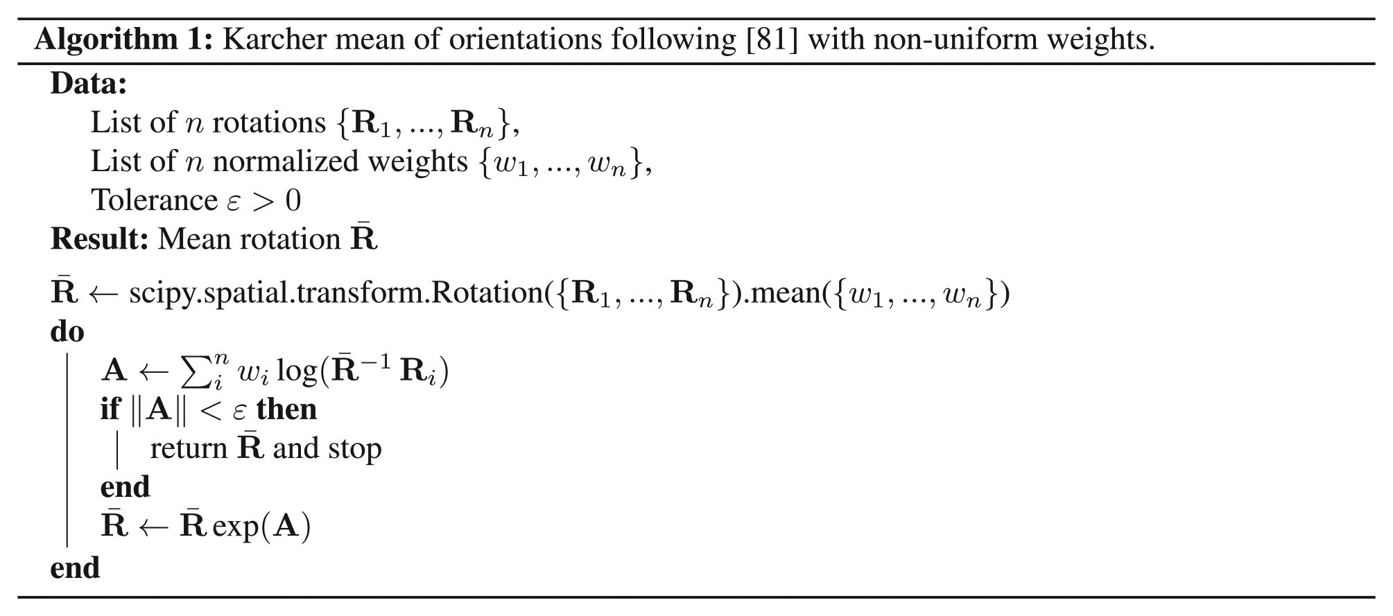
3.2.2. Interpolation of rotations

Rotations are elements of the special orthogonal group $\mathrm{SO}(3)$ which can be used to describe the orientation of a coordinate system relative to a reference coordinate system. In computer graphics, several heuristic and efficient algorithms are used to interpolate between two or multiple successive rotations, see Shoemake [72] and Dam et al. [73]. Interpolation algorithms for more than two rotations, derived from an engineering point of view and resulting in simple, yet not globally useful metrics and approximations, are given by Gramkow [74], Hartley et al. [75], and Markley et al. [76]. Connections between those algorithms and metrics on $\mathrm{SO}(3)$ are given by Hartley et al. [75] and Huynh [77]. Several interpolation methods [78–83] treat the space of rotations as Lie groups and manifolds and are mainly based on the Karcher [84] mean. Hereafter, rotation fields are interpolated based on the weighted Karcher mean specified in Algorithm 1 which extends the algorithm of Manton [81] by a set of normalized weights and a start value which is calculated with the algorithm of Markley et al. [76], implemented in Virtanen et al. [85].

Algorithm 1: Karcher mean of orientations following [81] with non-uniform weights.

Data:   List of n rotations $\{{\mathbf{R}}_1,...,{\mathbf{R}}_n\},$   List of n normalized weights $\{w_{\mathrm{I}},...,w_n\},$   Tolerance $\epsilon >0$ Result: Mean rotation $\overline{\mathbf{R}}$ $\overline{\mathbf{R}}\leftarrow$ scipy.spatial.transform.Rotation $\left(\{{\mathbf{R}}_1,...,{\mathbf{R}}_n\}\right).$ mean $(\{w_{\mathrm{I}},...,w_n\})$ do   $\mathbf{A}\leftarrow \sum _i^n{w}_i\log \left({\overline{\mathbf{R}}}^{-1}{\mathbf{R}}_i\right)$  if $\Vert \mathbf{A}\Vert <\epsilon$ then    return $\overline{\mathbf{R}}$ and stop  end   $\overline{\mathbf{R}}\leftarrow \overline{\mathbf{R}}$ exp $\left(\mathbf{A}\right)$ end

3.2.3. Interpolation of structure

The structure of a second-order fiber-orientation tensor within an eigensystem is encoded by two scalars. A popular redundancy-free visualization of this variety of the structure is the fiber-orientation triangle [86, 87], e.g., used in the works [88, 89]. The classification of structurally differing second-order fiber-orientation tensors in terms of the fiber-orientation triangle is based on the ordering convention

$${\lambda }_1\ge {\lambda }_2\ge {\lambda }_3,$$

(23)

see Bauer and Böhlke [55] for a detailed discussion. Any second-order orientation tensor can be represented by a pair $({\lambda }_1,{\lambda }_2)$ , which is connected to a point inside the orientation triangle and by one of the mappings ${\mathbf{Q}}_j$ .

The structure information of second-order fiber-orientation tensors or diffusion tensors is characterized by two or three independent invariants, respectively. Eigenvalues ${\lambda }_i$ with $i\in \{1,2,3\}$ are not common to encode the structure of diffusion tensors. Instead, one of two sets of invariant structure features is commonly used to describe diffusion tensors [41, 44, 50]. These sets are labeled $\{K_1,K_2,K_3\}$ and $\{R_1,R_2,R_3\}$ with $K_1$ also known as apparent diffusion coefficient (ADC), $R_2$ also known as fractional anisotropy (FA) [34], and $K_3=R_3$ called mode. Relations between the features $K_i$ and $R_i$ and explicit formulas are given by Gahm et al. [44]. In the next section, we follow the idea of using tensor components within a special coordinate system, the potentially unique eigensystem, to interpolate fourth-order fiber-orientation tensors. This idea follows the description of second-order tensors in terms of eigenvalues ${\lambda }_i$ with $i\in \{1,2,3\}$ .

4. Interpolation of fourth-order fiber-orientation tensors

4.1. Eigensystem-based parametrization

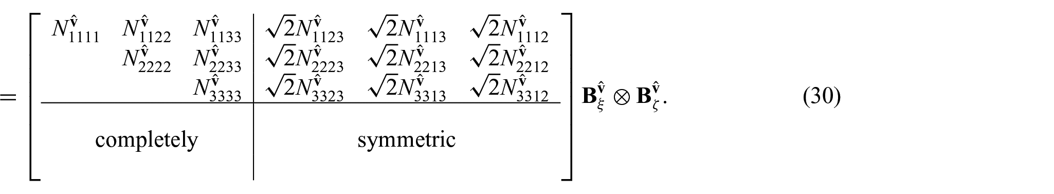
We transfer the interpolation strategy of separating orientation and structure to fourth-order fiberorientation tensors. Therefore, we use the parametrization of Bauer and Böhlke [55], which separates information on orientation and structure. The orientation information is represented in terms of an eigensystem and the structure information in terms of tensor components. These tensor components are represented in the Kelvin–Mandel notation, explicitly introduced by Mandel [90], originating from Thomson [91] and also known as the normalized Voigt notation. The Kelvin–Mandel notation uses a six-dimensional basis spanned by $\left\{{\mathbf{B}}_{\xi }\right\}$ for $\xi \in \{1,2,3,4,5,6\}$ and enables compact matrix representations of fourth-order tensors, while maintaining algebraic tensor properties [92–96]. For details on the basis ${\mathbf{B}}_{\xi }$ , the reader is referred to Mehrabadi and Cowin [92, equation (3.1)] or Bauer and Böhlke [55, equation (37)]. A completely symmetric fourth-order tensor $\mathbb{N}$ in the Kelvin–Mandel notation expressed in tensor components in an arbitrary coordinate system reads as

$$\mathbb{N}=N_{\mathrm{ijkl}}{\mathbf{e}}_i\otimes {\mathbf{e}}_j\otimes {\mathbf{e}}_k\otimes {\mathbf{e}}_l,$$

(24)

$$=\left[\begin{array}{cccccc}{N}_{1111}\hfill & N_{1122}\hfill & N_{1133}\hfill & \sqrt{2}{N}_{1123}\hfill & \sqrt{2}{N}_{1113}\hfill & \sqrt{2}{N}_{1112}\hfill \\ \multicolumn{1}{c}{}& N_{2222}\hfill & N_{2233}\hfill & \sqrt{2}{N}_{2223}\hfill & \sqrt{2}{N}_{2213}\hfill & \sqrt{2}{N}_{2212}\hfill \\ \multicolumn{1}{c}{}& \hfill & N_{3333}\hfill & \sqrt{2}{N}_{3323}\hfill & \sqrt{2}{N}_{3313}\hfill & \sqrt{2}{N}_{3312}\hfill \\ \hfill & \mathrm{completely}\hfill & \hfill & \hfill & \mathrm{symmetric}\hfill & \hfill \end{array}\right]{\mathbf{B}}_{\xi }\otimes {\mathbf{B}}_{\xi },$$

(25)

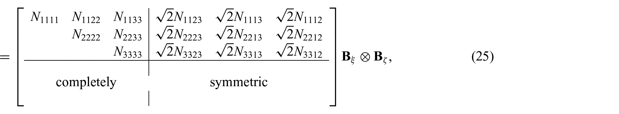
Bauer and Böhlke [55, equations (40) and (53)]. Given a fixed eigensystem $\left\{{\hat{\mathbf{v}}}_i\right\}$ , any fourth-order fiber-orientation tensor can be parametrized following Bauer and Böhlke [55, equations (59) and (60)] by

$$\mathbb{N}(\mathbf{N},d_1,...,d_9)={\mathbb{N}}^{\mathrm{iso}}+\frac{6}{7}\mathrm{sym}(\mathrm{dev}\left(\mathbf{N}\right)\otimes \mathbf{I})+\mathbb{F}(d_1,...,d_9)$$

(26)

with a potentially triclinic fourth-order deviator

$$\begin{array}{c}\mathbb{F}(d_1,...,d_9)=\hfill \\ \left[\begin{array}{cccccc}-(d_1+d_2)\hfill & d_1\hfill & d_2\hfill & -\sqrt{2}(d_4+d_5)\hfill & \sqrt{2}{d}_6\hfill & \sqrt{2}{d}_8\hfill \\ \multicolumn{1}{c}{}& -(d_1+d_3)\hfill & d_3\hfill & \sqrt{2}{d}_4\hfill & -\sqrt{2}(d_6+d_7)\hfill & \sqrt{2}{d}_9\hfill \\ \multicolumn{1}{c}{}& \hfill & -(d_2+d_3)\hfill & \sqrt{2}{d}_5\hfill & \sqrt{2}{d}_7\hfill & -\sqrt{2}(d_8+d_9)\hfill \\ \multicolumn{1}{c}{}& \mathrm{completely}\hfill & \hfill & \hfill & \mathrm{symmetric}\hfill & \hfill \end{array}\right]{\mathbf{B}}_{\xi }^{\hat{\mathbf{v}}}\otimes {\mathbf{B}}_{\zeta }^{\hat{\mathbf{v}}}\hfill \end{array}$$

(27)

and the Kelvin–Mandel basis $\{{\mathbf{B}}_{\xi }^{\hat{\mathbf{v}}}\}$ with $\xi \in \{1,2,3,4,5,6\}$ spanned in the fixed eigensystem $\left\{{\hat{\mathbf{v}}}_{\mathbf{i}}\right\}$ with $i\in \{1,2,3\}$ , and, e.g., the fourth basis vector in equation (27) being ${\mathbf{B}}_4^{\hat{\mathbf{v}}}=\sqrt{2}/2({\hat{\mathbf{v}}}_2\otimes {\hat{\mathbf{v}}}_3+{\hat{\mathbf{v}}}_3\otimes {\hat{\mathbf{v}}}_2)$ . The operator $\mathrm{sym}(·)$ projects onto the completely symmetric part of a tensor, and the operator $\mathrm{dev}(·)$ extracts the deviatoric part of a tensor [60]. The specific linear invariant decomposition in equation (26) is motivated by decomposition of elasticity tensors [67, 97, 98] and the following observation. When applied to fiber-orientation tensors of fourth order, the tensors’ central symmetry, i.e., complete index symmetry, causes one of the two irreducible second-order subspaces to vanish, if the decomposition operators are chosen appropriately. The invariance of the linear decomposition ensures that the transformation rules of the individual components are known and allows to decompose a tensor $\mathbb{N}$ into structure and orientation. The number of structure parameters ${\lambda }_1,{\lambda }_2$ and $d_i$ for $i\in \{1,2,...9\}$ is eleven and adds up with the three parameters defining $\left\{{\hat{\mathbf{v}}}_i\right\}$ , i.e., the orientation of $\mathbf{N}$ , to fourteen, which is the degree of freedom of a fourth-order fiber-orientation tensor. Material symmetry constraints, which arise naturally, e.g., in the context of closure approximations, reduce the number of degrees of freedom and lead to simplified parametrizations [54]. For example, orthotropic fourth-order fiber-orientation tensors are parametrized by

$${\mathbb{N}}^{\mathrm{ortho}}(\mathbf{N},d_1,d_2,d_3)=\mathbb{N}(\mathbf{N},d_1,d_2,d_3,0,0,0,0,0,0)$$

(28)

following Bauer and Böhlke [55, equation (76)].

The selection of the decomposition is significantly motivated by the experience of the authors involved. Alternative decompositions are given by, e.g., the spectral decomposition [91] which is utilized in section 4.4.2, to determine the material symmetry class of a given tensor, or the Clebsch–Gordan formalism [99, 100], also known as joined invariant decomposition.

4.2. New method: Interpolation of tensor components within the eigensystem

Based on the parametrization in equation (26), we introduce a new decomposition-based method for the interpolation of fourth-order fiber-orientation tensors in Algorithm 2. In a nutshell, this algorithm defines the interpolation of the structural information as a weighted average of tensor components within the tensors respective eigensystems. In detail, Algorithm 2 proposes to interpolate $\mathbf{n}$ fourth-order fiber-orientation tensors $\{{\mathbb{N}}_1,...,{\mathbb{N}}_n\}$ by a weighted average of their (unique) tensor components obtained within their individual, possibly non-unique, eigensystems $\{{\{{\mathbf{v}}_i^{\mathrm{u}}\}}_1,...,\{{\mathbf{v}}_i^{\mathrm{u}}{\}}_n\}$ and represent the resulting average of the tensor components in an interpolated coordinate system, obtained by interpolation of the individual eigensystems. The interpolation of the orientation information in terms of the eigensystems on one hand and the structural information in terms of the tensor components on the other hand are independent. In consequence, our proposal specifies the interpolation of the structural information and might be combined with any interpolation method for rotations to interpolate the eigensystems. One possible choice of the interpolation method of the eigensystems ${〈〈·〉〉}_{\mathrm{so}(3)}$ is given in Algorithm 1 and is used throughout this work.

Algorithm 2: Linear interpolation of unique tensor components of fourth-order fiber-orientation tensors within their eigensystems.

Data:   List of n fourth-order fiber-orientation tensors $\{{\mathbb{N}}_1,...,{\mathbb{N}}_n\}$   List of n normalized weights $\{w_{\mathrm{l}},...,w_n\},$   List of n possibly non-unique eigensystems $\{{\left\{{\mathbf{v}}_i^{\mathrm{u}}\right\}}_1...,{\left\{{\mathbf{v}}_i^{\mathrm{u}}\right\}}_n\}$   Weight-based interpolation method on $\mathrm{SO}\left(3\right)$ depicted by ${〈〈·〉〉}_{\mathrm{so}(3)}$ Result: Interpolated fourth-order fiber-orientation tensor $\overline{\mathbb{N}}$ for $i=1;i\le n;i=i+1$ do   Rotate ${\mathbb{N}}_i$ into ${\left\{{\mathbf{v}}_j^{\mathrm{u}}\right\}}_i$ leading to ${\left(N_{\mathrm{mnop}}^{{\mathbf{v}}^{\mathrm{u}}}\right)}_i$ $({\mathbf{v}}_m^{\mathrm{u}}\otimes {\mathbf{v}}_n^{\mathrm{u}}\otimes {\mathbf{v}}_o^{\mathrm{u}}\otimes {\mathbf{v}}_p^{\mathrm{u}}{)}_i$ end $\left\{{\overline{\mathbf{v}}}_j\right\}\leftarrow {〈〈{\left\{{\mathbf{v}}_j^{\mathrm{u}}\right\}}_i〉〉}_{\mathrm{SO}\left(3\right)}$ $\overline{\mathbb{N}}\leftarrow \sum _i^n{w}_i{\left(N_{\mathrm{mnop}}^{{\mathbf{v}}^{\mathrm{u}}}\right)}_i{\overline{\mathbf{v}}}_m\otimes {\overline{\mathbf{v}}}_n\otimes {\overline{\mathbf{v}}}_o\otimes {\overline{\mathbf{v}}}_p$ return $\overline{\mathbb{N}}$

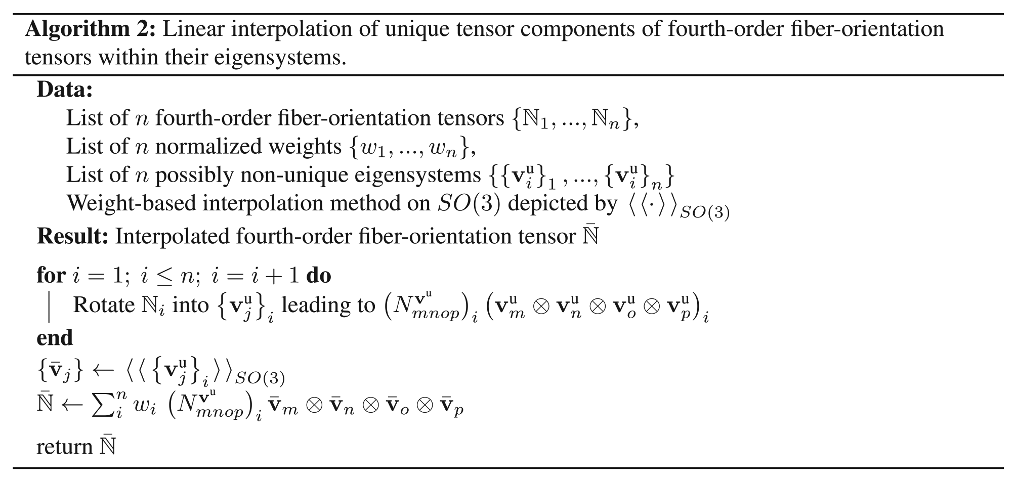
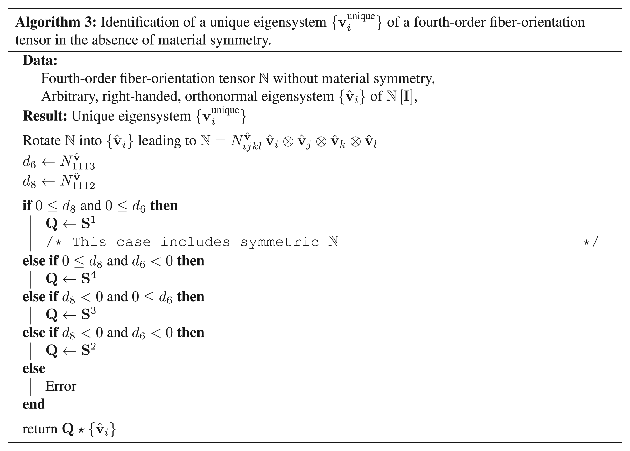
In the absence of any material symmetry, i.e., if all tensors which are to be interpolated are triclinic, each of these tensors possesses a unique eigensystem $\left\{{\mathbf{v}}_i^{\mathrm{u}}\right\}$ and a unique set of structural parameters in terms of equation (26). Since a fiber-orientation tensor, which is obtained from flow simulations or measured experimentally, will be effected by noise, the tensor is unlikely to possess exact material symmetry. In consequence, most applications are concerned with triclinic tensors with unique eigensystem and we refer to operating on such tensors as the “general case.” For this general case, we specify a procedure to obtain a unique eigensystem in section 4.3. On the contrary, if a fiber-orientation tensor shows (partial) material symmetry, it might not possess a unique eigensystem. Since identification of an eigensystem and consequently a unique set of parameters in terms of equation (26) are crucial for the new interpolation algorithm, we present such an identification procedure in section 4.4.1 discussing all edge cases.

To illustrate, why the identification of the eigensystem, in both the general case and the edge cases, require further investigation, it is worth noting that Bauer and Böhlke [55] developed the eigensystem-based parametrization in equation (26) to study the variety of fourth-order fiber-orientation tensors and used the parametrization as the starting point. Similarly, Bauer et al. [54] use the parametrization as the starting point for microstructure optimization in terms of semi-definite programming on fiber-orientation tensors. Starting with the parametrization fixes the eigensystem a priori. This is why the ambiguity of the four possible eigensystems of a second-order tensor in the absence of material symmetry elaborated in section 3.2.1 is not discussed by Bauer and Böhlke [55] or Bauer et al. [54]. Using the parametrization as a starting point, implicitly selects one of the possible eigensystems of the tensor of interest. This is even the case for material symmetries, e.g., isotropy for which the number of eigensystems is infinite, as any coordinate system represents a valid eigensystem.

4.3. General case: The unique eigensystem in the absence of material symmetry

We investigate fiber-orientation tensors in the absence of material symmetry, i.e., we concentrate on triclinic tensors. Let the tensor components of a triclinic fourth-order fiber-orientation tensor $\mathbb{N}$ be given in any of the four possible eigensystems $\left\{{\hat{\mathbf{v}}}_i\right\}$ of its second-order information, reading

$$\mathbb{N}=N_{\mathrm{ijkl}}{\mathbf{e}}_i\otimes {\mathbf{e}}_j\otimes {\mathbf{e}}_k\otimes {\mathbf{e}}_l$$

(29)

$$=\left[\begin{array}{cccccc}{N}_{1111}^{\hat{\mathbf{v}}}\hfill & N_{1122}^{\hat{\mathbf{v}}}\hfill & N_{1133}^{\hat{\mathbf{v}}}\hfill & \sqrt{2}{N}_{1123}^{\hat{\mathbf{v}}}\hfill & \sqrt{2}{N}_{1113}^{\hat{\mathbf{v}}}\hfill & \sqrt{2}{N}_{1112}^{\hat{\mathbf{v}}}\hfill \\ \multicolumn{1}{c}{}& N_{2222}^{\hat{\mathbf{v}}}\hfill & N_{2233}^{\hat{\mathbf{v}}}\hfill & \sqrt{2}{N}_{2223}^{\hat{\mathbf{v}}}\hfill & \sqrt{2}{N}_{2213}^{\hat{\mathbf{v}}}\hfill & \sqrt{2}{N}_{2212}^{\hat{\mathbf{v}}}\hfill \\ \multicolumn{1}{c}{}& \hfill & N_{3333}^{\hat{\mathbf{v}}}\hfill & \sqrt{2}{N}_{3323}^{\hat{\mathbf{v}}}\hfill & \sqrt{2}{N}_{3313}^{\hat{\mathbf{v}}}\hfill & \sqrt{2}{N}_{3312}^{\hat{\mathbf{v}}}\hfill \\ \multicolumn{1}{c}{}& \mathrm{completely}\hfill & \hfill & \hfill & \mathrm{symmetric}\hfill & \hfill \end{array}\right]{\mathbf{B}}_{\xi }^{\hat{\mathbf{v}}}\otimes {\mathbf{B}}_{\zeta }^{\hat{\mathbf{v}}}.$$

(30)

The action of elements in the orthotropic symmetry group ${\mathcal{S}}^{\mathrm{ortho}}$ , listed in equations (20) and (21), on the tensor $\mathbb{N}$ , expressed in the coordinate system $\left\{{\hat{\mathbf{v}}}_i\right\}$ , is given by

$${\mathbf{S}}_1^{\mathrm{ortho}}★\mathbb{N}=\mathbb{N},$$

(31)

$${\mathbf{S}}_2^{\mathrm{ortho}}★\mathbb{N}=\left[\begin{array}{cccccc}{N}_{1111}^{\hat{\mathbf{v}}}\hfill & N_{1122}^{\hat{\mathbf{v}}}\hfill & N_{1133}^{\hat{\mathbf{v}}}\hfill & \sqrt{2}{N}_{1123}^{\hat{\mathbf{v}}}\hfill & -\sqrt{2}{N}_{1113}^{\hat{\mathbf{v}}}\hfill & -\sqrt{2}{N}_{1112}^{\hat{\mathbf{v}}}\hfill \\ \multicolumn{1}{c}{}& N_{2222}^{\hat{\mathbf{v}}}\hfill & N_{2233}^{\hat{\mathbf{v}}}\hfill & \sqrt{2}{N}_{2223}^{\hat{\mathbf{v}}}\hfill & -\sqrt{2}{N}_{2213}^{\hat{\mathbf{v}}}\hfill & -\sqrt{2}{N}_{2212}^{\hat{\mathbf{v}}}\hfill \\ \multicolumn{1}{c}{}& \hfill & N_{3333}^{\hat{\mathbf{v}}}\hfill & \sqrt{2}{N}_{3323}^{\hat{\mathbf{v}}}\hfill & -\sqrt{2}{N}_{3313}^{\hat{\mathbf{v}}}\hfill & -\sqrt{2}{N}_{3312}^{\hat{\mathbf{v}}}\hfill \\ \multicolumn{1}{c}{}& \mathrm{completely}\hfill & \hfill & \hfill & \mathrm{symmetric}\hfill & \hfill \end{array}\right]{\mathbf{B}}_{\xi }^{\hat{\mathbf{v}}}\otimes {\mathbf{B}}_{\zeta }^{\hat{\mathbf{v}}},$$

(32)

$${\mathbf{S}}_3^{\mathrm{ortho}}★\mathbb{N}=\left[\begin{array}{cccccc}{N}_{1111}^{\hat{\mathbf{v}}}\hfill & N_{1122}^{\hat{\mathbf{v}}}\hfill & N_{1133}^{\hat{\mathbf{v}}}\hfill & -\sqrt{2}{N}_{1123}^{\hat{\mathbf{v}}}\hfill & \sqrt{2}{N}_{1113}^{\hat{\mathbf{v}}}\hfill & -\sqrt{2}{N}_{1112}^{\hat{\mathbf{v}}}\hfill \\ \multicolumn{1}{c}{}& N_{2222}^{\hat{\mathbf{v}}}\hfill & N_{2233}^{\hat{\mathbf{v}}}\hfill & -\sqrt{2}{N}_{2223}^{\hat{\mathbf{v}}}\hfill & \sqrt{2}{N}_{2213}^{\hat{\mathbf{v}}}\hfill & -\sqrt{2}{N}_{2212}^{\hat{\mathbf{v}}}\hfill \\ \multicolumn{1}{c}{}& \hfill & N_{3333}^{\hat{\mathbf{v}}}\hfill & -\sqrt{2}{N}_{3323}^{\hat{\mathbf{v}}}\hfill & \sqrt{2}{N}_{3313}^{\hat{\mathbf{v}}}\hfill & -\sqrt{2}{N}_{3312}^{\hat{\mathbf{v}}}\hfill \\ \multicolumn{1}{c}{}& \mathrm{completely}\hfill & \hfill & \hfill & \mathrm{symmetric}\hfill & \hfill \end{array}\right]{\mathbf{B}}_{\xi }^{\hat{\mathbf{v}}}\otimes {\mathbf{B}}_{\zeta }^{\hat{\mathbf{v}}},$$

(33)

$${\mathbf{S}}_4^{\mathrm{ortho}}★\mathbb{N}=\left[\begin{array}{cccccc}{N}_{1111}^{\hat{\mathbf{v}}}\hfill & N_{1122}^{\hat{\mathbf{v}}}\hfill & N_{1133}^{\hat{\mathbf{v}}}\hfill & -\sqrt{2}{N}_{1123}^{\hat{\mathbf{v}}}\hfill & \sqrt{2}{N}_{1113}^{\hat{\mathbf{v}}}\hfill & -\sqrt{2}{N}_{1112}^{\hat{\mathbf{v}}}\hfill \\ \multicolumn{1}{c}{}& N_{2222}^{\hat{\mathbf{v}}}\hfill & N_{2233}^{\hat{\mathbf{v}}}\hfill & -\sqrt{2}{N}_{2223}^{\hat{\mathbf{v}}}\hfill & \sqrt{2}{N}_{2213}^{\hat{\mathbf{v}}}\hfill & -\sqrt{2}{N}_{2212}^{\hat{\mathbf{v}}}\hfill \\ \multicolumn{1}{c}{}& \hfill & N_{3333}^{\hat{\mathbf{v}}}\hfill & -\sqrt{2}{N}_{3323}^{\hat{\mathbf{v}}}\hfill & \sqrt{2}{N}_{3313}^{\hat{\mathbf{v}}}\hfill & -\sqrt{2}{N}_{3312}^{\hat{\mathbf{v}}}\hfill \\ \multicolumn{1}{c}{}& \mathrm{completely}\hfill & \hfill & \hfill & \mathrm{symmetric}\hfill & \hfill \end{array}\right]{\mathbf{B}}_{\xi }^{\hat{\mathbf{v}}}\otimes {\mathbf{B}}_{\zeta }^{\hat{\mathbf{v}}},$$

(34)

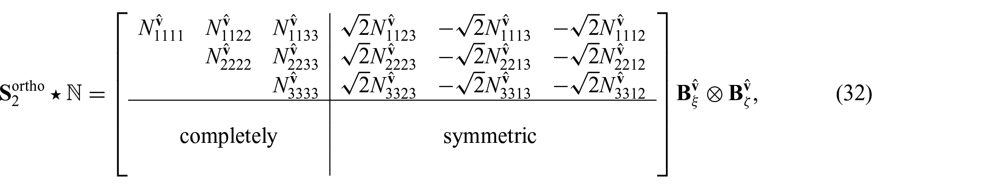
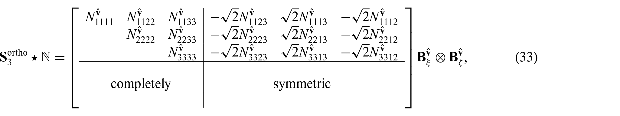
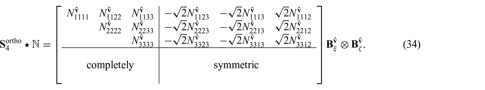
Comparing the tensor components in equations (31) to (34) reveals that the non-trivial rotations within the group ${\mathcal{S}}^{\mathrm{ortho}}$ change signs of two columns within the upper right quadrant and due to symmetry also two rows in the lower left quadrant of the coefficient matrix each. This is not surprising, if we remember the eigensystems associated with each of the group elements, which are defined in equations (15) to (18). For example, the rotation ${\mathbf{S}}_2^{\mathrm{ortho}}$ which transforms the eigensystem $\left\{{\hat{\mathbf{v}}}_i\right\}$ into the one given in equation (16) by changing the signs of the second and third base vectors ${\hat{\mathbf{v}}}_2$ and ${\hat{\mathbf{v}}}_3$ leads to a change of sign in the second and third column of the upper right quadrant in equation (32). From this observation, we conclude that introducing a sign-convention, i.e., binary constraints, on two suitable tensor components defines a unique eigensystem $\left\{{\mathbf{v}}_i^{\mathrm{unique}}\right\}$ of fourth-order fiber-orientation tensors which have weaker material symmetry than orthotropy.

Although this convention might seem a bit arbitrary at first, it is quite common to use conventions on invariants to select features of an eigensystem. In the case of second-order fiber-orientation tensors $\mathbf{N}$ , the sorting convention on the eigenvalues in equation (23) is well established and defines the order of the eigenvectors in ${\left\{{\mathbf{v}}_i\right\}}_j$ for each $j\in \{1,2,3,4\}$ . The directions of the axes of the $j\mathrm{th}$ eigensystem ${\left\{{\mathbf{v}}_i\right\}}_j$ of a tensor $\mathbf{N}$ are based on conventions upon the size of invariants, namely the eigenvalues ${\lambda }_1$ and ${\lambda }_2$ . We define a unique eigensystem of a given fourth-order fiber-orientation tensor $\mathbb{N}$ in the absence of material symmetry based on signs of invariant tensor components in this unique eigensystem itself. Since any convention necessarily requires a decision, we decide for the components $N_{1113}^{\hat{\mathbf{v}}}=d_6$ and $N_{1112}^{\hat{\mathbf{v}}}=d_8$ to be non-negative. Any other choice leads to an equivalent set of parameters combined with an eigensystem that differs from the one we have chosen by the sign/direction of specific axes. Studying the variety of planar fourth-order fiber-orientation tensors, Bauer and Böhlke [64] required the parameter $d_8$ to be non-negative to eliminate a redundancy within the identified admissible parameter space. This implicit definition of $\{{\mathbf{v}}_i^{\mathrm{unique}}\}$ is motivated by the observations in equations (31) to (34) and leads to Algorithm 3. Among the four possible eigensystems, Algorithm 3 selects the one, which leads to non-negative values of $d_6$ and $d_8$ in the parametrization in equation (26).

Algorithm 3: Identification of a unique eigensystem $\left\{{\mathbf{v}}_i^{\mathrm{unique}}\right\}$ of a fourth-order fiber-orientationtensor in the absence of material symmetry.

Data:   Fourth-order fiber-orientation tensor $\mathbb{N}$ without material symmetry,   Arbitrary, right-handed, orthonormal eigensystem $\left\{{\hat{\mathbf{v}}}_{\mathrm{i}}\right\}\mathrm{of}\mathbb{N}\left[\mathbf{I}\right],$ Result: Unique eigensystem $\left\{{\mathbf{v}}_i^{\mathrm{unique}}\right\}$ Rotate $\mathbb{N}$ into $\left\{{\hat{\mathbf{v}}}_{\mathrm{i}}\right\}$ leading to $\mathbb{N}=N_{\mathrm{ijkl}}^{\hat{\mathbf{v}}}{\hat{\mathbf{v}}}_i\otimes {\hat{\mathbf{v}}}_j\otimes {\hat{\mathbf{v}}}_k\otimes {\hat{\mathbf{v}}}_l$ $d_6\leftarrow N_{1113}^{\hat{\mathbf{v}}}$ $d_8\leftarrow N_{1112}^{\hat{\mathbf{v}}}$ if $0\le d_8\mathrm{and}0\le d_6$ then    $\mathbf{Q}\leftarrow {\mathbf{S}}^1$   /* This case includes symmetric $\mathbb{N}$       */ else if $0\le d_8\mathrm{and}{d}_6<0$ then   $\mathbf{Q}\leftarrow {\mathbf{S}}^4$ else if $d_8<0\mathrm{and}0\le d_6$ then   $\mathbf{Q}\leftarrow {\mathbf{S}}^3$ else if $d_8<0\mathrm{and}{d}_6<0$ then   $\mathbf{Q}\leftarrow {\mathbf{S}}^2$ Else  Error end return $\mathbf{Q}★\left\{{\hat{\mathbf{v}}}_i\right\}$

4.4. Edge cases: Identification of eigensystem and structural parameters in the presence of material symmetry

4.4.1. Implications of material symmetry on the uniqueness of the eigensystem

A unique eigensystem forms the basis for the decomposition-based interpolation method defined in section 4.2. However, in the presence of (partial) material symmetry, the unique eigensystem approach fails. We illustrate this with the example of cubic fourth-order fiber-orientation tensors.

For potentially noise-affected measurements of fiber-orientation tensors of real microstructures, the presence of material symmetries is rather unlikely, especially in the case of large reference volumes. In such cases, even a slight asymmetry of the fibers’ arrangement will lead to a triclinic fiber-orientation tensor. However, analysis of dilute microstructures or artificially generated microstructures may include fiber-orientation tensors which posses some kind of material symmetry. Therefore, we aim at associating given components of a fourth-order fiber-orientation tensor, with a unique set of parameters ${\lambda }_i$ for $i\in \{1,2\}$ and $d_i$ for $i\in \{1,2,3,4,5,6,7,8,9\}$ combined with a unique eigensystem or at least a limited number of possible eigensystems. The authors are aware of alternative methods for the interpolation of directional information of lower-order tensors, such as unique projector representations [29, 56], but in this work, we focus on eigensystem-based approaches. With decomposition-based interpolation methods, it is possible to separate the interpolation of the obtained structural parameters ${\lambda }_i$ and $d_i$ from the interpolation of the potentially non-unique eigensystems and to take the ambiguity of the latter into account. This reasoning might be illustrated by considering interpolation of multiple fiber-orientation tensors of which exactly one is isotropic, i.e., ${\mathbb{N}}^{\mathrm{iso}}$ and the others have a countable number of possible eigensystems. In this case, the interpolation method might include the structural information of the isotropic tensor but exclude its arbitrary eigensystem in the interpolation of the eigensystems. Similarly, countable ambiguities, such as the fourfold ambiguity of the eigensystem of any orthotropic fourth-order fiber-orientation tensor, might be considered for the interpolation of the eigensystems, but the interpolation of the structural parameters is not affected by the symmetry itself, as those parameters are not influenced by the choice of the eigensystem. However, there are cases in which a more detailed examination is necessary to obtain a unique set of structural parameters. These cases are motivated by the following example and discussed in the next sections.

Example: The cubic edge case. Of special interest are those cases, where the second-order information is more symmetric than the fourth-order information. We start by investigating a group of fourth-order fiber-orientation tensors which are not isotropic but contract to the isotropic second-order fiber-orientation tensor. Several subspaces of fiber-orientation tensors with this property exist. Examples are the space of cubic fourth-order fiber-orientation tensors as well as a line within the admissible transversely isotropic fourth-order fiber-orientation tensors with vanishing second-order contribution. If the second-order part $\mathbf{N}=\mathbb{N}\left[\mathbf{I}\right]$ of a fourth-order fiber-orientation tensor $\mathbb{N}$ is isotropic, the eigensystem of $\mathbf{N}$ is indeterminate as all three eigenvalues are equal, and hence, any coordinate system is eigensystem of the second-order tensor. However, not every coordinate system is eigensystem of the corresponding fourth-order fiber-orientation tensor. In consequence, fourth-order fiber-orientation tensors exist, which have an eigensystem, that is defined by fourth-order information. The simplest example of a whole group of fiber-orientation tensors with this property is given by cubic fourth-order fiber-orientation tensors. To the best of the authors’ knowledge, cubic fourth-order fiber-orientation tensors have not been presented in the literature before. Using the parametrization in equation (26), cubic fiber-orientation tensors, which only have one degree of freedom, can be represented by

$${\mathbb{N}}^{\mathrm{cubic}}\left(d_1\right)={\mathbb{N}}^{\mathrm{iso}}+\mathbb{F}(d_1,d_1,d_1,0,0,0,0,0,0)$$

(35)

and contract to isotropic second-order fiber-orientation tensors, i.e., ${\mathbb{N}}^{\mathrm{cubic}}\left(d_1\right)\left[\mathbf{I}\right]=1/3\mathbf{I}={\mathbf{N}}^{\mathrm{iso}}$ holds. Details on admissible cubic fourth-order fiber-orientation tensors are given in Appendix 1. A visualization of five cubic fiber distributions associated with tensors along the one-dimensional admissible space is given in Figure 4. The minimum value of $d_1$ corresponds to $\mathrm{cubify}({\mathbf{e}}_1)$ with the operator $\mathrm{cubify}(·)$ applying all $24$ symmetry transformations of the cubic symmetry group $[{\mathbf{S}}_i]$ with $i\in [1,2,...,24]$ to given quantity. In consequence, the operator $\mathrm{cubify}(\mathbf{n})$ returns a list of $24$ elements with each element representing ${\mathbf{S}}_i★\mathbf{n}$ for $i\in [1,2,...,24]$ , e.g., $\mathrm{cubify}({\mathbf{e}}_1)=[{\mathbf{S}}_1★{\mathbf{e}}_1,...,{\mathbf{S}}_{24}★{\mathbf{e}}_1]$ . The maximum value $d_1$ corresponds to $\mathrm{cubify}({\mathbf{e}}_1+{\mathbf{e}}_2+{\mathbf{e}}_3)$ . All other states may be realized by applying all cubic symmetry transformations to a vector obtained by linear interpolation between ${\mathbf{e}}_1$ and ${\mathbf{e}}_1+{\mathbf{e}}_2+{\mathbf{e}}_3$ . For reference, the isotropic state is characterized by the value $d_1=0$ . The appeal and at the same time a challenge of the parametrization equation (26) is the definition of the potentially triclinic fourth-order part $\mathbb{F}$ in terms of tensor components in the eigensystem of the corresponding second-order fiber-orientation tensor. In consequence, once an eigensystem is chosen, this system is eigensystem of both the second- and fourth-order part of the solution. This demonstrates the suitability of the parametrization equation (26) if we start with structural parameters ${\lambda }_i$ for $i\in \{1,2\}$ and $d_i$ for $i\in \{1,2,3,4,5,6,7,8,9\}$ and an a priori defined eigensystem. However, within the present work, we start with tensor components of fourth-order fiber-orientation tensors which are to be interpolated. Therefore, we seek algorithms to obtain as much information towards a unique eigensystem of a given tensor, as possible. As these algorithms might depend on the symmetry of the given tensor itself, we start with identifying the material symmetry class of a given tensor’s second- and fourth-order parts.

Figure 4.

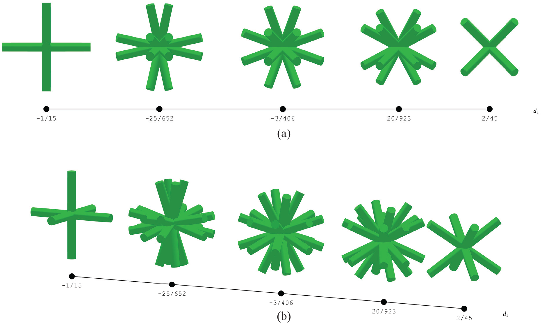
Examples of cubic fiber arrangements along the one-dimensional parameter space of cubic fourth-order fiber-orientation tensors: (a) first view and (b) second view.

4.4.2. Identification of the material symmetry

We try to identify the material symmetry class of given tensors based on the multiplicity of eigenvalues, following Bòna et al. [101] who summarize extensive research on the identification of material symmetry and a natural basis, i.e., an eigensystem, of given linear elastic stiffnesses, see Thomson [91], Mehrabadi and Cowin [92], Cowin and Mehrabadi [93], Rychlewski [97], Fedorov [102], Walpole [103], Rychlewski [104, 105], Yang et al. [106], Sutcliffe [107], and Browaeys and Chevrot [108]. Therefore, we define eigenvalues ${\mathrm{\Lambda }}_{\xi }$ of a fourth-order tensor $\mathbb{B}$ as solution to the spectral problem $\mathbb{B}[\mathbf{V}]=\mathrm{\Lambda }\mathbf{V}$ , with the associated second-order eigentensor $\mathbf{V}\in \mathrm{Sy}{\mathrm{m}}_2$ and the space of symmetric second-order tensors $\mathrm{Sy}{\mathrm{m}}_2$ . We start with investigating the second-order fiber-orientation tensor $\mathbf{N}=\mathbb{N}\left[\mathbf{I}\right]$ associated with a given fourth-order fiber-orientation tensor $\mathbb{N}$ . A second-order tensor in general belongs to one out of three groups of material symmetries, depending on the multiplicity of its eigenvalues. Following Bauer [109, chapter 3] the three cases of one, two, and three distinct eigenvalues can be associated with groups of material symmetries, the associated fourth-order fiber-orientation tensor might belong to, see Table 1. To give an example, a fourth-order fiber-orientation tensor which contracts to a second-order tensor with three distinct eigenvalues can either be triclinic, monoclinic, or orthotropic but not more symmetric, like transversely isotropic, trigonal, tetragonal, cubic, or isotropic. However, even a triclinic fourth-order fiber-orientation tensor might contract to an isotropic second-order tensor, as the fourth-order information is able to encode granular directional information which might not be expressible in a coarse directional measure of second order. The identification of the material symmetry of fiber-orientation tensors is easier than the one of linear elastic stiffnesses [97, 101, 110], as the algebraic structure of fiber-orientation tensors is limited to one constant isotropic part, one irreducible second-order tensor, and one irreducible fourth-order tensor [55], due to the tensor’s index symmetry. In contrast, less symmetric elasticity tensors contain two isotropic constants and two irreducible second-order tensors. Nevertheless, we adopt the reasoning of Bòna et al. [101, 110] and count distinct eigenvalues of irreducible fourth-order tensors $\mathrm{dev}\left(\mathbb{N}\right)=\mathbb{F}(d_1,d_2,...,d_9)$ in equation (26) to identify the tensors material symmetry class. Based on the multiplicity of eigenvalues of a fourth-order fiber-orientation tensor’s irreducible part, five groups of material symmetry classes can be identified following Table 2. In order to apply the selection procedure depicted in Table 2 on eigenvalues obtained from tensor components of a given fiber-orientation tensor, the eigenvalues have to be rounded to a suitable numerical precision, before counting. Having identified, or at least narrowed, the material symmetry class of a given fourth-order fiber-orientation tensor using Table 2, we are now interested in retrieving eigensystem information from the fourth-order’s deviator. Therefore, we inspect the deviator’s eigentensors.

Table 1.

Mapping of the multiplicity of the eigenvalues of a second-order fiber-orientation tensor $\mathbf{N}=\mathbb{N}\left[\mathbf{I}\right]$ to possible material symmetry classes of the associated fourth-order fiber-orientation tensor $\mathbb{N}$ .

Distinct eigenvalues ${\lambda }_i$ of $\mathbf{N}$	Multiplicities of ${\lambda }_i$	Possible material symmetries of $\mathbb{N}$
1	3	any
2	2, 1	any but the isotropic or cubic one
3	1, 1, 1	either orthotropic, monoclinic, or triclinic

Table 2.

Mapping of the multiplicity of the eigenvalues of a fourth-order fiber-orientation tensor to its possible symmetry classes.

Distinct eigenvalues of $\mathrm{dev}\left(\mathbb{N}\right)$	Multiplicities of the eigenvalues	Possible material symmetry classes
1	6	isotropic
3	3, 2, 1	cubic
4	2, 2, 1, 1	transversely isotropic, trigonal
5	2, 1, 1, 1, 1	tetragonal
6	1, 1, 1, 1, 1, 1	orthotropic, monoclinic, triclinic

4.4.3. Cubic symmetry

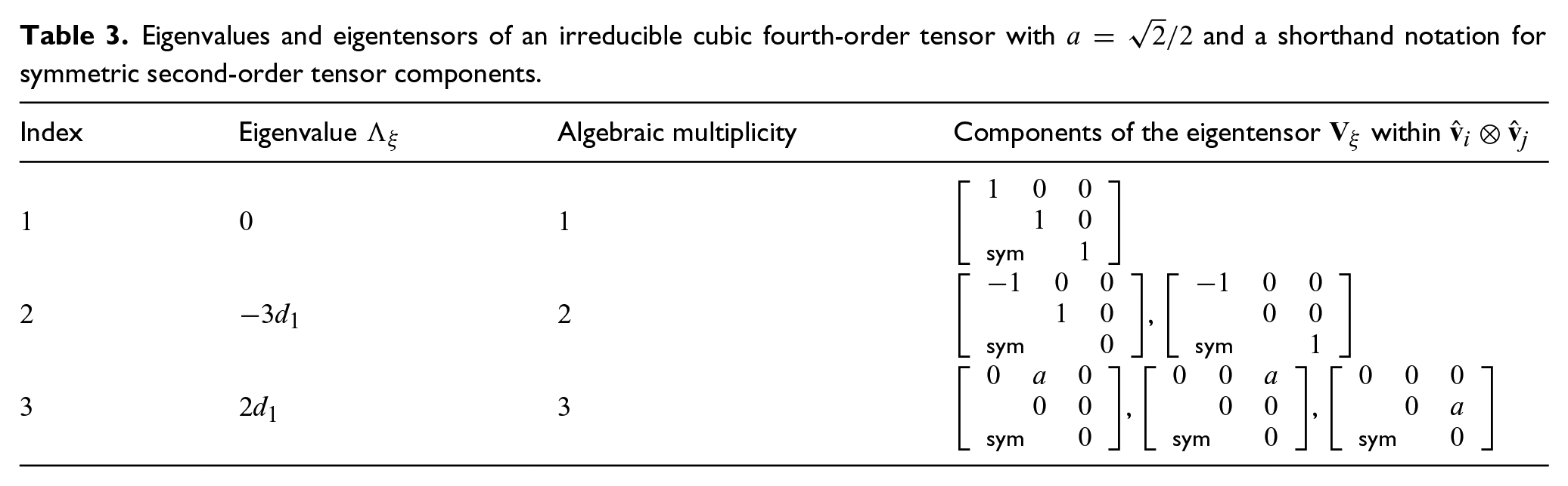
We start with cubic material symmetry. Table 3 shows the eigenvalues, their algebraic multiplicity and corresponding eigentensors of a cubic deviator $\mathrm{dev}{\left(\mathbb{N}\right)}^{\mathrm{cubic}}$ represented in an eigensystem ${\hat{\mathbf{v}}}_i\otimes {\hat{\mathbf{v}}}_j$ . We observe that the coefficient matrices of those eigentensors, which correspond to the eigenvalue of multiplicity two, have diagonal shape within the eigensystem. In consequence, we can derive an eigensystem candidate of a cubic deviator $\mathrm{dev}\left(\mathbb{N}\right)$ from the spectral decomposition of its eigentensors which correspond to its twofold eigenvalue. This spectral decomposition will yield a rotation matrix specifying one eigensystem candidate as well as eigenvalues of known value. This observation defines an identification strategy for the cubic parameters as well as one of the 24 eigensystems of a cubic fourth-order fiber-orientation tensor implemented in the code [111]. Having identified one eigensystem, generator expressions for the cubic symmetry group, e.g., following Weber et al. [71] and Bauer [109], can be used to identify the remaining 23 eigensystems. The non-uniqueness of the eigensystem of tensors of strong material symmetry as in the cubic case states a challenge for the interpolation of the eigensystem orientation.

Table 3.

Eigenvalues and eigentensors of an irreducible cubic fourth-order tensor with $a=\sqrt{2}/2$ and a shorthand notation for symmetric second-order tensor components.

Index	Eigenvalue ${\mathrm{\Lambda }}_{\xi }$	Algebraic multiplicity	Components of the eigentensor ${\mathbf{V}}_{\xi }$ within ${\hat{\mathbf{v}}}_i\otimes {\hat{\mathbf{v}}}_j$
$1$	$0$	$1$	$\left[\begin{array}{ccc}1\hfill & 0\hfill & 0\hfill \\ \multicolumn{1}{c}{}& 1\hfill & 0\hfill \\ \multicolumn{1}{c}{\mathrm{sym}}& \hfill & 1\hfill \end{array}\right]$
$2$	$-3d_1$	$2$	$\left[\begin{array}{ccc}-1\hfill & 0\hfill & 0\hfill \\ \multicolumn{1}{c}{}& 1\hfill & 0\hfill \\ \multicolumn{1}{c}{\mathrm{sym}}& \hfill & 0\hfill \end{array}\right],\left[\begin{array}{ccc}-1\hfill & 0\hfill & 0\hfill \\ \multicolumn{1}{c}{}& 0\hfill & 0\hfill \\ \multicolumn{1}{c}{\mathrm{sym}}& \hfill & 1\hfill \end{array}\right]$
$3$	$2d_1$	$3$	$\left[\begin{array}{ccc}0\hfill & a\hfill & 0\hfill \\ \multicolumn{1}{c}{}& 0\hfill & 0\hfill \\ \multicolumn{1}{c}{\mathrm{sym}}& \hfill & 0\hfill \end{array}\right],\left[\begin{array}{ccc}0\hfill & 0\hfill & a\hfill \\ \multicolumn{1}{c}{}& 0\hfill & 0\hfill \\ \multicolumn{1}{c}{\mathrm{sym}}& \hfill & 0\hfill \end{array}\right],\left[\begin{array}{ccc}0\hfill & 0\hfill & 0\hfill \\ \multicolumn{1}{c}{}& 0\hfill & a\hfill \\ \multicolumn{1}{c}{\mathrm{sym}}& \hfill & 0\hfill \end{array}\right]$

4.4.4. Transversely isotropic, trigonal, or tetragonal symmetry: Step one

A physical quantity which is either transversely isotropic, trigonal, or tetragonal has a preferred axis. We follow the convention of Bauer [109, Chapter 3] and select any parametrization such that this axis is parallel to ${\hat{\mathbf{v}}}_1$ . Irreducible tensors of fourth-order following this convention are given for the three material symmetries of interest in the work [109, equations (3.28), (3.29), and (3.30)]. Tables of eigenvalues and eigentensors of these irreducible tensors are given in Appendix 4 in Tables A1–A3. We observe that for any of these three material symmetries, one of the deviator’s eigentensors has diagonal shape within the coordinate system ${\hat{\mathbf{v}}}_i\otimes {\hat{\mathbf{v}}}_j$ and in addition has constant eigenvalues, which values are known a priori. The direction associated with the eigenvalue of maximum absolute value of the aforementioned eigentensor is the preferred axis, i.e., ${\hat{\mathbf{v}}}_1$ . Given a fourth-order fiber-orientation tensor, which eigenvalue pattern matches with either the transversely isotropic, trigonal, or tetragonal pattern in Table 2, we identify the preferred axis as follows. We calculate a spectral decomposition of the deviator’s eigentensor which corresponds to the eigenvalue triplet of values two, negative one and negative one. As the sign of eigentensors is arbitrary, the sign of the eigenvalues of an eigentensor is arbitrary as well. Therefore, some care has to be taken on the signs and orders of the eigenvectors of the eigentensor of interest, resulting in implementation details which are documented in the code [111]. Nevertheless, the spectral analysis of the eigentensor with the specific eigenvalue signature yields a transformation into a coordinate system, which first axis is aligned with the preferred axis of the given fiber-orientation tensor. It should be noted that aligning the first axis ${\hat{\mathbf{v}}}_1$ with the preferred axis of the material symmetry does not fit the frequently applied ordering convention on eigenvalues of the associated second-order fiber-orientation tensor resulting from equation (23) combined with equation (14). For an oblate transversely isotropic fiber-orientation tensor of second-order, the preferred axis corresponds to an eigenvector associated with an eigenvalue which is smaller than the remaining two eigenvalues. If the fourth-order fiber-orientation tensor which is to be analyzed is transversely isotropic, we are done, the obtained coordinate system is one valid eigensystem and structural parameters can be directly obtained from the tensor components in this coordinate system. However, if the tensor components on the obtained coordinate system indicate that the inspected fiber-orientation tensor is not continuous rotational symmetric with respect to the ${\hat{\mathbf{v}}}_1$ axis, an additional analysis step is necessary.

4.4.5. Trigonal or tetragonal symmetry: Step two

In contrast to the continuous rotational symmetry of transversely isotropic quantities, trigonal and tetragonal quantities are symmetric with respect to rotations of specific angles around a preferred axis only.

The preferred axis has been identified as the first axis ${\hat{\mathbf{v}}}_1$ of a coordinate system obtained in the first analysis step demonstrated in section 4.4.4. Starting from this coordinate system, we need to identify a rotation around the axis ${\hat{\mathbf{v}}}_1$ which transforms the deviator of the fiber-orientation tensor of interest into its representation within one of its eigensystems, see equation (50) or equation (44). As the axis of the rotation of interest is known, we seek for an angle only. One way to obtain this angle is to deploy a minimization algorithm minimizing the norm of those tensor components which vanish in the eigensystem representation. As the trigonal and tetragonal material symmetries can be distinguished based on the eigenvalue signature of the analyzed fourth-order fiber-orientation tensors deviator, the bounds of the angle during the optimization process can be limited to specific values.

If the analyzed tensor is trigonal, the angle takes a value between 0 and 60 degrees. Once the angle minimizing the target function is identified, the parameters $d_3$ and $d_9$ can be directly obtained from the tensor components within the identified eigensystem. As discussed in Appendix 3, the sign of the parameter $d_9$ might be restricted to negative values in order to get unique sets of parameters. If the parameter $d_9$ in the optimized eigensystem is positive, the eigensystem might be consecutively transformed by ${\mathbf{S}}_2^{\mathrm{ortho}}$ , defined in equation (20).

If the analyzed tensor is tetragonal, rotations between 0 and 90 degrees have to be considered during the optimization process. Having obtained tensor components within the optimized coordinate system, one additional step is necessary to obtain a unique set of parameters. Rotation of 45 degrees around the axis ${\hat{\mathbf{v}}}_1$ the value of the parameter $d_3$ . Therefore, we can restrict admissible values of $d_3$ to those fulfilling the condition $d_3\le -d_1/4$ . If this condition is not met from a candidate $d_3^{\mathrm{candidate}}$ , the actual parameter $d_3$ is obtained by $d_3=-d_1/2-d_3^{\mathrm{candidate}}$ and the eigensystem is obtained by rotating the optimized eigensystem candidate by another 45 degrees around ${\hat{\mathbf{v}}}_1$ .

4.4.6. Orthotropic symmetry

For a given orthotropic fourth-order fiber-orientation tensor ${\mathbb{N}}^{\mathrm{ortho}}$ , we seek a unique set of parameters and eigensystems to uniquely describe the given tensor in terms of the parametrization in equation (28). As already stated before, the second-order part $\mathbf{N}={\mathbb{N}}^{\mathrm{ortho}}\left[\mathbf{I}\right]$ is either isotropic, transversely isotropic, or orthotropic. For each of these three symmetries of the second-order part, we define a strategy to obtain a unique set of parameters.

First, if the second-order part $\mathbf{N}$ is orthotropic, its four eigensystems are the eigensystems of ${\mathbb{N}}^{\mathrm{ortho}}$ and due to the symmetry, no additional specification of the eigensystem based on fourth-order information is possible. Second, if the second-order part $\mathbf{N}$ is transversely isotropic, its spectral decomposition yields one of its infinitesimal many eigensystems. All eigensystems of the second-order part share a preferred axis and only differ by rotations around this axis. Bauer and Böhlke [55, Figure 2] visualized and discussed the redundancy within the parameter space of transversely isotropic second-order fiber-orientation tensors. It is common to parametrize second-order fiber-orientation tensors within the so-called fiber-orientation triangle [55, 86]. The transversely isotropic subspace within the fiber-orientation triangle contains two edges, connected by the isotropic second-order tensor. We associate these two edges with two groups of second-order fiber-orientation tensors, prolate and oblate ones. Two eigenvalues of a transversely isotropic second-order fiber-orientation tensor coincide and differ from the remaining eigenvalue. If the twofold eigenvalue is smaller than the remaining eigenvalue, the tensor is called prolate, otherwise oblate. Prolate tensors are located within the fiber-orientation triangle along the edge between the isotropic and the unidirectional states. Oblate tensors are located along the edge between the isotropic and the planar isotropic states. We follow a common convention and associate the rotational axis of prolate tensors with the axis ${\mathbf{v}}_1$ and the rotational axis of oblate tensors with the axis ${\mathbf{v}}_3$ . These associations result from the convention of sorting the eigenvalues by decreasing value. In consequence, finding eigensystems of the given orthotropic fourth-order fiber-orientation tensor is reduced to finding an angle of rotation around an axis specified by its second-order part. If the second-order part is prolate, this axis is the axis ${\mathbf{v}}_1$ , otherwise it is the axis ${\mathbf{v}}_3$ . As the given fourth-order fiber-orientation tensor is orthotropic, the upper right /lower left quadrant within the Kelvin–Mandel notation contains only zeros and the semi-norm, i.e., the subadditive and absolute homogeneous expression

$$\delta (\mathbb{N})=\sqrt{\sum _{(\mathrm{ijkl})\in \mathcal{M}}{N}_{\mathrm{ijkl}}^2}\mathrm{with}\mathcal{M}=\{1123,1113,1112,2223,2213,2212,3323,3313,3312\}$$

(36)

with $\mathbb{N}=N_{\mathrm{ijkl}}{\mathbf{e}}_i\otimes {\mathbf{e}}_j\otimes {\mathbf{e}}_k\otimes {\mathbf{e}}_l$ vanishes within one of its eigensystems. Therefore, the rotational angle of interest can be identified by minimizing $\delta (\mathbb{N})$ . Figures 5 and 6 show the dependency of the orthotropic fourth-order parameters $d_1,d_2,$ and $d_3$ on the rotation angle $\varphi$ in case of two randomly chosen orthotropic fourth-order fiber-orientation tensors with prolate and oblate second-order part, respectively. In order to get unique parameter sets, we introduce the following conventions. We require $d_2\le d_1$ for orthotropic fourth-order fiber-orientation tensors with a prolate transversely isotropic second-order part and $d_3\le d_2$ for those with oblate second-order part. If the conventions on the size of $d_1,d_2,$ and $d_3$ are not met, an additional rotation of 90 degrees is necessary to obtain suitable parameters and an eigensystem.

Figure 5.

Identification of a unique parameter set of a randomly selected and randomly oriented orthotropic fourth-order fiber-orientation tensor $\mathbb{N}({\lambda }_1=0.5,{\lambda }_2=0.25,d_1=0.05,d_2=0.033,d_3=0.011)$ with a prolate transversely isotropic second-order part, being rotated around the preferred axis of rotation of its second-order part. Values ${\hat{d}}_1(\varphi ),{\hat{d}}_2(\varphi )$ , and ${\hat{d}}_3(\varphi )$ are extracted for every angle $\varphi$ .

Figure 6.

Identification of a unique parameter set of a randomly selected and randomly oriented orthotropic fourth-order fiber-orientation tensor $\mathbb{N}({\lambda }_1=0.4583,{\lambda }_2=0.4583,d_1=-0.05,d_2=-0.01,d_3=-0.02)$ with an oblate transversely isotropic second-order part, being rotated around the preferred axis of rotation of its second-order part. Values ${\hat{d}}_1(\varphi ),{\hat{d}}_2(\varphi )$ , and ${\hat{d}}_3(\varphi )$ are extracted for every angle $\varphi$ .

Third, if the second-order part $\mathbf{N}$ is isotropic, it does not contain orientational information and its spectral decomposition yields a random coordinate system. However, the spectral decomposition of a generic orthotropic fourth-order deviator in Table A4 indicates that a spectral decomposition of the tensors deviatoric fourth-order part contains orientational information. Two eigentensors, those with index five and six in Table A4, have a diagonal shape within the eigensystem, we are after. Therefore, we call these two eigentensors diagonal, hereafter. Within a first step, we iterate over the eigentensors obtained by a spectral decomposition of the orthotropic fourth-order fiber-orientation tensor of interest ${\mathbb{N}}^{\mathrm{ortho}}$ and identify any of the diagonal tensors by being associated with a non-vanishing eigenvalue of ${\mathbb{N}}^{\mathrm{ortho}}$ and not having the sorted eigenvalue triplet $[-1/\sqrt{2},0,1/\sqrt{2}]$ . A spectral decomposition of this diagonal eigentensor yields an eigensystem candidate. However, due to the isotropy of the second-order part, we require a convention on the parameters $d_1,d_2,$ and $d_3$ and decide for

$$d_3\le d_2\le d_1.$$

(37)

In the next step, we transform the fourth-order deviator into the eigensystem candidate and within this candidate system extract candidates for the parameters $d_1,d_2,$ and $d_3$ . We then sort the parameters to fit the convention in equation (37) and apply the same sorting permutation onto the eigenvectors of the eigensystem candidate to obtain an eigensystem of ${\mathbb{N}}^{\mathrm{ortho}}$ in which the parameters $d_1,d_2,$ and $d_3$ follow the convention in equation (37). The three strategies to obtain eigensystems and unique parameter sets of orthotropic fourth-order fiber-orientation tensors are implemented in the code [111].

4.4.7. Triclinic and monoclinic symmetries

Algorithm 3 defines a unique eigensystem for any triclinic fourth-order fiber-orientation tensor with orthotropic second-order part. This algorithm is not successful, if the second-order part of the tensor of interest is isotropic or transversely isotropic. However, those cases are rare, as a sufficient number of fibers are required to obtain triclinic fourth-order information and those fibers would have to state an arrangement which in second-order precision is more symmetric than orthotropic. Fiber-orientation tensors which fulfill this constraint can be easily constructed. However, the authors assume that such states are rarely found in real fiber arrangement. We refrain from developing an algorithm to cover this edge case. We deploy a similar argumentation for the monoclinic case.

4.4.8. Summary on edge cases

Following section 4.3, we can assign a unique eigensystem to any fourth-order fiber-orientation tensor, if the tensor (or equivalently its deviatoric parts of second and fourth orders) does not possess any (partial) material symmetry. If, in contrast, a fiber-orientation tensor does possess (partial) material symmetry, we might follow one of the strategies introduced in section 4.4 to identify a set of eigensystems in which the tensor components fulfill specific requirements. These requirements contain conventions on signs and relations of tensor components. The structural information is completely encoded within the unique set of tensor components within any of the eigensystems.

5. Application

5.1. Visualization and setup

Within the following sections, we apply the new interpolation algorithm (Algorithm 2) combined with the interpolation of rotations following Algorithm 1. We start with interpolation between two given fourth-order fiber-orientation tensors and advance towards the interpolation of planar tensor fields with linear varying weights obtained by triangulation. Within the following figures, fourth-order fiber-orientation tensors are visualized in terms of truncated fiber-orientation distribution functions approximated by leading second- and fourth-order tensors [64, equation (31)]. Negative values are indicated by red color. Alternative visualization methods for fourth-order fiber-orientation tensors, i.e., quartic and glyph plots, are discussed and compared to each other in Appendix 5.

5.2. Interpolation between two fiber-orientation tensors

Figure 7 visualizes the interpolation of two fiber-orientation tensors which differ solely by a rotation. The figure contains two views on five truncated fiber-orientation distributions each. Each distribution represents a fourth-order fiber-orientation tensor. The fiber-orientation tensors visualized by the left- and right-most distributions in Figure 7 are given, and the remaining bodies represent interpolated orientation tensors. Weights are linearly varying between the given orientation states.

Figure 7.

Interpolation between two fiber-orientation tensors which differ solely by a rotation, depicted by two views (a) first view and (b) second view. The visualized bodies represent truncated fiber-orientation distribution functions approximated by leading second- and fourth-order tensors [64, equation (31)]. Green color indicates the positive values, and red color indicates the negative values. The left- and right-most bodies are given; the others are interpolated. The given fiber-orientation tensors are orthotropic and defined by ${\mathbb{N}}^{\mathrm{ortho}}({\lambda }_1=0.5,{\lambda }_2=0.25,d_1=0.05,d_2=0.033,d_3=0.011)$ .

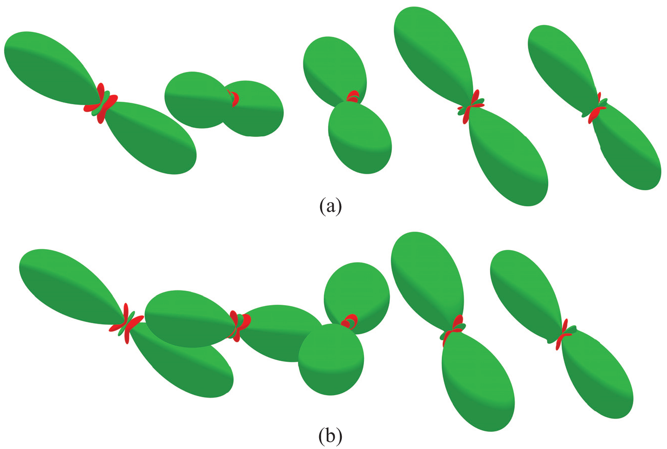
In Figure 8, linearly weighted interpolation between two cubic fourth-order fiber-orientation tensors is shown. Again, tensors are visualized in terms of truncated distribution functions and the left- and right-most tensors are given; the others are interpolated. Qualitative comparisons between the discrete fiber realizations in Figure 4 and the fiber-orientation tensors visualized in Figure 8 reveal the encoding of the preferred fiber direction. It should be noted, however, that the concrete fiber arrangements in Figure 4 represent only one concrete realization each, whereas the fiber-orientation tensors visualized in Figure 8 represent a variety of fiber arrangements on average.

Figure 8.

Interpolation between two extreme cubic fiber-orientation tensors with homogeneous eigensystems, depicted by two views (a) first view and (b) second view. The visualized bodies represent truncated fiber-orientation distribution functions approximated by leading second- and fourth-order tensors [64, equation (31)]. Green color indicates the positive values, and red color indicates the negative values. The left- and right-most bodies are given; the others are interpolated. The left-most body represents a cubic fiber-orientation tensor parametrized by ${\mathbb{N}}^{\mathrm{cubic}}(d_1=-1/15)$ whereas the left-most body is defined by ${\mathbb{N}}^{\mathrm{cubic}}(d_1=2/45)$ .

Figure 9 as well as Figure 10 show interpolation between two randomly selected triclinic fourth-order fiber-orientation tensors. The visualizations follow the pattern of Figures 7 and 8. The unique eigensystems based on Algorithm 3 of the given fiber-orientation tensors within Figure 9 differ only slightly, leading to a small rotation among the interpolated states. In contrast, the unique eigensystems of the given fiber-orientation tensors in Figure 10 differ by a large angle in any relative measure within the space of rotations, i.e., $\mathrm{SO}(3)$ . As both given fiber-orientation tensors are characterized by relatively large values of the first eigenvalue of $\mathbf{N}$ , i.e., ${\lambda }_1$ , the visualizations of both tensors are quite similar. The large rotation, induced by the strongly differing eigensystems, might not fit expectations associated with flow fields between the left- and right-most tensors and therefore might be interpreted as an artifact of the interpolation method.

Figure 9.

Interpolation between two randomly selected triclinic fourth-order fiber-orientation tensors, depicted by two views (a) first view and (b) second view. The visualized bodies represent truncated fiber-orientation distribution functions approximated by leading second- and fourth-order tensors [64, equation (31)]. Green color indicates the positive values, and red color indicates the negative values. The left- and right-most bodies are given; the others are interpolated. The left-most fiber-orientation tensor is approximately defined by $\mathbb{N}({\lambda }_1=0.7205,{\lambda }_2=0.1983,d_1=0.0337,d_2=-0.0283,d_3=0.0009,d_4=-0.0038,d_5=-0.0005,$ $d_6=0.0107,d_7=0.0007,d_8=0.0312,d_9=-0.0471)$ , whereas the rightmost tensor is approximately given by $\mathbb{N}({\lambda }_1=0.8449,{\lambda }_2=0.1173,d_1=-0.0287,d_2=-0.0681,d_3=0.0119,$ $d_4=0.0001,d_5=-0.0013,d_6=0.0193,$ $d_7=0.0012,d_8=0.016,d_9=-0.0235)$ .

Figure 10.

Interpolation between two randomly selected triclinic fourth-order fiber-orientation tensors, depicted by two views (a) first view and (b) second view. In contrast to Figure 9, the directions of the first axis of the unique eigensystems of the tensors to be interpolated differ significantly. The visualized bodies represent truncated fiber-orientation distribution functions approximated by leading second- and fourth-order tensors [64, equation (31)]. Green color indicates the positive values, and red color indicates the negative values. The left- and right-most bodies are given; the others are interpolated. The orientation of the unique eigensystem of a given tensor is specified by a rotation vector $\mathbf{n}$ . This vector defines a transformation of a random global coordinate system $\{{\mathbf{e}}_i\}$ into the tensors unique eigensystem. The angle of rotation in radians is encoded by the norm of the vector $\mathbf{n}$ . The left-most fiber-orientation tensor is approximately defined by $\mathbb{N}({\lambda }_1=0.923,{\lambda }_2=0.0564,d_1=-0.0612,d_2=-0.0871,d_3=0.0186,d_4=0.0011,$ $d_5=-0.0,d_6=0.0021,d_7=0.0016,d_8=0.0084,d_9=-0.0083)$ combined with a rotation vector $\mathbf{n}=[-2.83948,-0.90225,-0.88844]{\mathbf{e}}_i$ , whereas the rightmost tensor is approximately given by $\mathbb{N}({\lambda }_1=0.764,{\lambda }_2=0.1566,d_1=0.0067,d_2=-0.0378,d_3=0.0051,d_4=-0.0017,d_5=0.0096,$ $d_6=0.0134,d_7=-0.0068,d_8=0.0249,d_9=-0.0073)$ combined with a rotation vector $\mathbf{n}=[-0.50503,2.1305,-0.41356]{\mathbf{e}}_i$ .

5.3. Interpolation of transversely isotropic fourth-order structures on a planar grid

The subspace of transversely isotropic fourth-order fiber-orientation tensor is two-dimensional [8, 52, 112]. Within this two-dimensional space, we select five orientation tensors as reference grid points. These five reference tensors are the unidirectional, planar, and isotropic fourth-order fiber-orientation tensors combined with two tensors $\mathbb{A}={\mathbb{N}}^{\mathrm{transv}}(\mathbf{N}={\mathbf{N}}^{\mathrm{iso}},d_3=1/60)$ and $\mathbb{B}={\mathbb{N}}^{\mathrm{transv}}(\mathbf{N}={\mathbf{N}}^{\mathrm{iso}},d_3=-1/90)$ , see the work [55, equations (69) and (70)]. The two latter fiber-orientation tensors contract to the isotropic second-order fiber-orientation tensor, for which any coordinate system acts as eigensystem. Figure 11 shows the reference grid points labeled by indices following Table 4 and interpolations based on linearly varying triangulated weights. The diagonal between the grid points (1, 1) and (5, 5) contains states which all have arbitrary eigensystems and divide the space of all transversely isotropic orientation states in prolate and oblate states.

Figure 11.

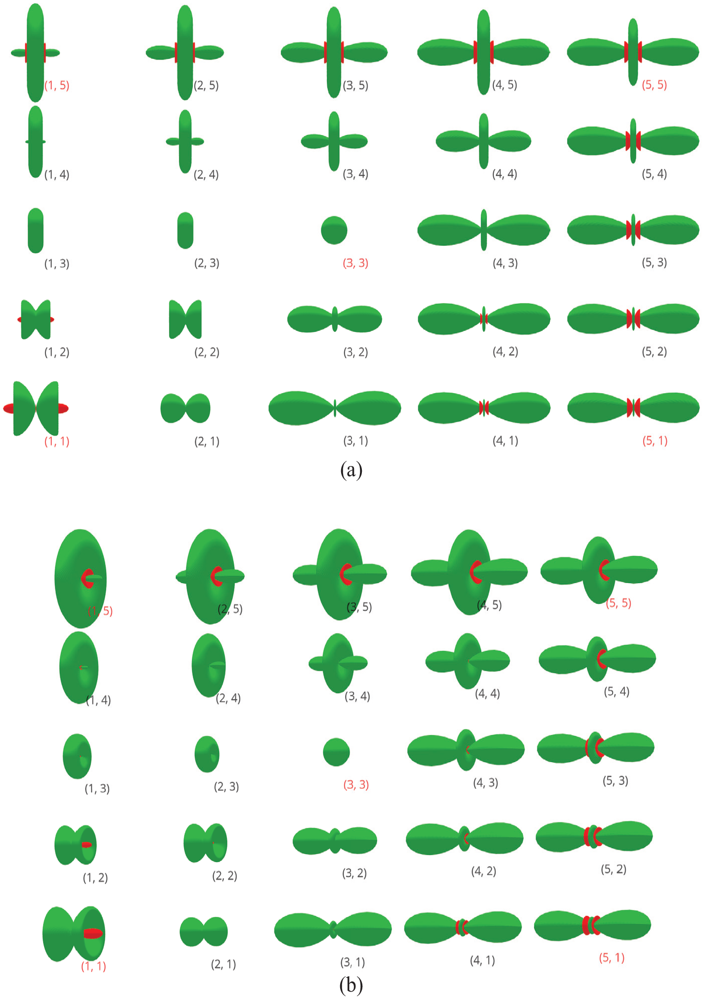
Interpolation problem of homogeneously aligned transversely isotropic fourth-order fiber-orientation tensor. Fiber-orientation tensor is represented as truncated fiber-orientation distribution function (FODF) approximations [64, equation (31)]. The FODF labeled in red are supporting grid points of the problem, whereas black labels indicate the interpolated FODF. Those FODFs which are nearly unidirectional, i.e., (4,2), (5,2), (3,1), (4,1), (5,1) are shrunk to fit into the figure. States on the diagonal, i.e., $(i,i)$ for $i\in \{1,2,3,4,5\}$ are isotropic in the sense of the second-order information $\mathbf{N}$ : (a) first view and (b) second view.

Table 4.

Mapping between indices in Figure 11 and transversely isotropic fourth-order fiber-orientation tensors.

Indices	Fiber-orientation tensor
(5,1)	Unidirectional
(1,5)	Planar isotropic
(3,3)	Isotropic
(5,5)	$\mathbb{A}$
(1,1)	$\mathbb{B}$

This missing definiteness leads to problems for decomposition-based interpolation methods as the orientation of eigensystems changes suddenly when passing this diagonal. The interpolated fiber-orientation tensors visualized in Figure 11 are obtained by linear interpolation of their tensor components within a given, homogeneous coordinate system. As the eigensystem identification procedure described in section 4.4.4, implemented in the computer code [111], is used, the transversely isotropic axes align throughout oblate and prolate orientation states. In consequence, the common ordering convention (equation (23)) for the eigenvalues of the contained second-order tensor does not hold.

5.4. Interpolation of measured fourth-order fiber-orientation tensors

The authors apply the new interpolation method defined in Algorithm 2 to a two-dimensional field of fiber-orientation tensors, measured by CT by Blarr et al. [113]. This problem consists of nine tensors which are nearly unidirectional. We obtain interpolation weights by triangulation and linear shape function. The resulting tensor field is visualized in Figure 12.

Figure 12.

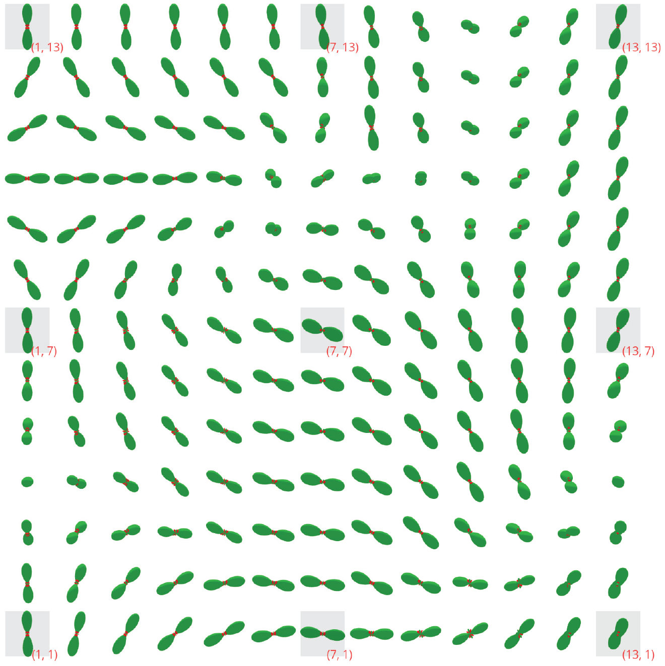
Interpolation of experimentally measured fiber-orientation tensors. The tensors are represented as truncated fiber-orientation distribution function (FODF) approximations [64, equation (31)] (see also Appendix 5). The supporting grid points of the problem are each indicated by a light gray box and red label. The remaining FODF representations are interpolated.

On the complete left edge, the right upper edge, and the lower right edge, we observe rotations larger than ninety degrees between two given grid points. This indicates that the orientation of the axis ${\mathbf{e}}_1$ of two neighboring fiber-orientation tensors changes. The observed large rotations are an intrinsic consequence of associating a fiber-orientation tensor with a coordinate system and subsequently interpolating the associated coordinate systems. As a consequence, the investigated interpolation method might not be suited for practical applications in its current formulation, as the subjective visual impression of the interpolated field might be artificially jumbled. Combination of the structural properties utilized in the new interpolation method with an orientation-less projector representation of the orientational information could lead to an interpolation method with improved visual impression for the problem at hand.

6. Conclusion

In this paper, we discuss the interpolation of fiber-orientation tensors on spatially discretized fields and distinguish interpolation from other problems such as averaging and disassembly. Motivated by decomposition-based interpolation methods for second-order fiber-orientation tensors, we present a new interpolation method for fiber-orientation tensors of order four. The presented interpolation method is built on an eigensystem-based parametrization, thereby naturally separating the interpolation of eigensystems and structural properties. The structural properties are encoded in terms of tensor components in the mentioned eigensystem. We discuss the difficulty of non-unique eigensystems in the presence of various partial material symmetries. This discussion starts with a convention which, in the absence of material symmetry, defines a unique eigensystem of a given triclinic fourth-order fiber-orientation tensor. For most combinations of material symmetries of the second- and fourth-order parts of a given fourth-order fiber-orientation tensor, we present algorithms and conventions to determine eigensystems as well as unique parameter combinations.

It should be mentioned that edge cases can be avoided using projector-based methods instead of the discussed eigensystem-based parametrization [29, 56, 57]. In the context of these edge case considerations, the groups of cubic, trigonal, and tetragonal fourth-order fiber-orientation tensors are explicitly given for the first time in terms of parametrizations and admissible parameter ranges, therefore extending the existing contributions [31, 54, 55, 64]. Furthermore, eigenvalues and eigentensors of irreducible structure tensors with cubic, transversely isotropic, trigonal, tetragonal as well as orthotropic material symmetry are presented. However, the numerous case distinctions, which are necessary in the presence of arbitrary material symmetries, show that the new interpolation method is only conditionally suitable for practical applications. This statement is the result of a detailed analysis of the underlying parametrization and can be generalized as follows. The parametrization of Bauer and Böhlke [55] is very well suited to generate or analyze realizations of fiber-orientation tensors starting from a defined eigensystem. However, if an eigensystem of a given fiber-orientation tensor is to be determined, difficulties arise on edge cases, as repeated eigenvalues lead to ambiguities discussed in section 4.4. We collect and compare visual representations of fourth-order fiber-orientation tensors in terms of truncated Fourier series, quartic plots, and tensor glyphs. The work at hand concludes with application of the new interpolation method.