A growth spin model is proposed for the modelling of the expansive growth and fibre remodelling of cell wall. The introduction of the growth spin allows to relax the perfectly bonding assumption in the kinematical growth, which provides a more sophisticated and flexible kinematical description for modelling the selective control and flexible regulation of anisotropic growth. Extended hardening laws are proposed for the growth and remodelling, respectively, aiming at further clarification of the dynamic balance between hardening and softening in a growing cell wall. The proposed model may shed a new light into the micro-structural interpretation of the “fictitious” intermediate (growth) configuration in the kinematical growth modelling of soft matter. A case study of the cell wall as a growing cylindrical wall is presented to demonstrate the proposed model. Spencer’s deviatoric stress tensor and its rate format are shown to play a key role in the modelling of the cell wall as a fibre-reinforced soft tissue.
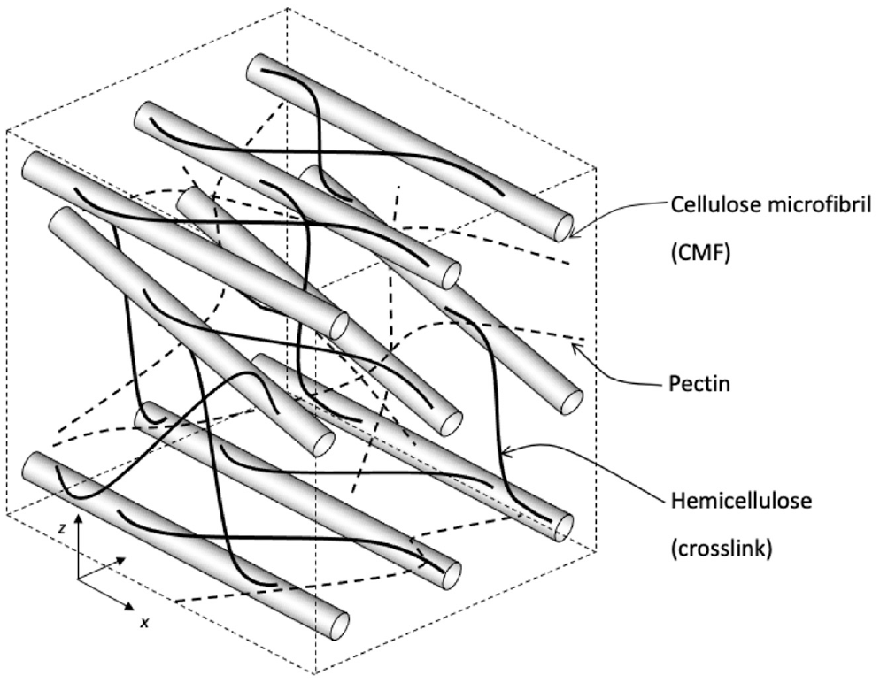
How cells expand despite the presence of cell walls is a central issue in plant biology [1–6]. The plant cell wall is a composite in which cellulose microfibrils (CMFs) are embedded into an amorphous matrix composed of hemicellulose, pectins, and proteins (see Figure 1). Microfibrils, several nanometres in width and many micrometres long, have a tensile strength similar to that of steel, and are relatively inert and inextensible in growth [7,8]. Neighbouring microfibrils tend to be roughly parallel, giving the cell wall a mat-like appearance and a distinct structural anisotropy similar to a laminated composite.
A schematic REV of cell wall showing distribution of cellulose microfibrils (CMFs), hemicelluloses, and pectins in a laminated material.
The cell wall is synthesised in an integrative effort: mobile cellulose synthesis complexes produce long, thin, strong, stiff CMFs at the cell surface, while matrix polysaccharides and glycoproteins are deposited to the cell surface via the secretory apparatus [4]. The newly deposited material may be transported through the wall matrix along the wall thickness direction and integrated into the existing microstructure [9,10]. Together, such a process of deposition, transport, and integration creates the volumetric growth of the wall.
However, wall synthesis without mechanical relaxation would only cause wall thickening [11,12]. To grow, plant cells must physically expand their restraining cell walls with the help of turgor pressure (about 5 bar) applied on its inner surface while satisfying wall yielding (or called wall loosening) threshold condition [3,13]. The wall yielding/loosening refers to a molecular modification of the wall network that results in relaxation of wall stress. Wall stress relaxation might result from scission of a stress-bearing crosslink or from sliding of such a crosslink along a scaffold; in both cases, it results in a reduction in wall stress without a substantial change in wall dimensions [2]. Therefore, in addition to the contribution from the volumetric growth, cell wall expansive growth has the contribution from the passively stress-driven irreversible isochoric in-plane expansion, which is analogues to the conventional viscoplasticity and may be considered playing a dominant and leading role in cell wall growth. Nevertheless, wall expansion without the matching volumetric growth inevitably results in wall thinning and eventually ruptures of material. Thus, the matching volumetric growth may be considered playing a supporting role to the wall expansion for maintaining stable wall geometry and strength.
Therefore, the cell wall must satisfy two contradictory requirements. It must be strong enough to resist mechanical stress (which may exceed (1000 bar)) generated by cell turgor pressure, and at the same time, it must be sufficiently compliant to permit irreversible wall expansion. Although it is widely accepted that the cell wall accommodates these requirements through its composite structure, the earliest molecular depictions of growing cell walls were offered as concept maps of how the composite components might be spatially arranged and connected to one another as hypothetical summaries rather than quantitative or predictive models [5].
By contrast, macroscopic phenomenological models provided both quantitative prediction and qualitative interpretation from the perspective of continuum theory. As a milestone, Lockhart [14] summarised a wide range of experimental data on wall extensibility in a formula, i.e., the well-known “Lockhart equation” which is a one-dimensional (1D) viscoplasticity-like model with a yield surface from the point of view of solid mechanics.
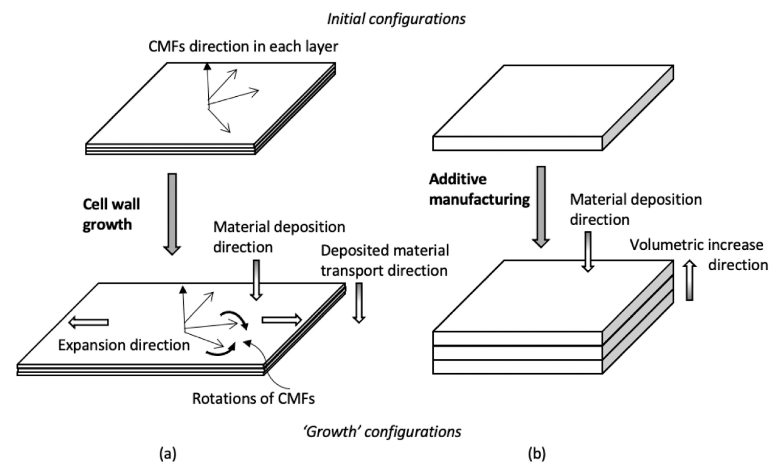
In principle, a three-dimensional (3D) growth model may be proposed using an elasto-viscoplasticity-like theoretical framework taking the Lockhart equation as its consistent volumetric/uniaxial format. Boudaoud [15] investigated the growth of isolated walled cells, where cell growth is similar to a perfectly plastic deformation. Dumais et al. [16] developed an anisotropic viscoplastic thin shell model of cell walls which was the first attempt at integrating mechanical deformation driven by the turgor pressure with new material deposition and transport. Huang et al. [17,18] proposed the finite strain fibre-reinforced models of cell wall growth which took into account the non-linear elasticity, the mechanical inelastic behaviour (e.g., viscoelastic behaviour which performs differently in loading and unloading), and the temperature-dependent growth driven by stress and sustained with new material deposition and transport. In consistency with the aforementioned biological postulates of cell wall growth [2–4,9,10], those phenomenological models [16,17] proposed a key assumption that cell wall expansive growth may be decomposed into (i) a directly stress-driven irreversible isochoric in-plane expansion and (ii) the associated out-of-plane volumetric growth achieved by material deposition, transport, and integration (see Figure 2(a)).
Cell wall growth compared with additive manufacturing (AM): (a) Cell wall material is schematically represented by a laminated composite material with one family of CMFs in each layer pointing to different directions. Cell wall growth includes the in-plane isochoric expansion (surface enlargement) and the matching volumetric growth maintaining a stable wall thickness. The volumetric growth results from the material deposition on the wall surface and the subsequent material transport in the same direction from the wall surface through the wall thickness. CMFs may (or may not) rotate depending on the stress distribution. (b) AM shows out-of-plane volumetric increase in a direction opposite to the direction of material deposition.
During the last decade, finite element method has been increasingly applied to cell wall growth modelling (see, e.g., Yanagisawa et al. [19] and the reviews [4,5]), which provided a computational tool to support the new experimental development using atomic force microscopy and X-ray scattering [20,21]. A number of publications [4,5,6,22–24] provided the extensive reviews about the recent progress on the multiscale modelling of cell wall and its growth from different points of view. The more general theories about the mathematical modelling of biological growth and remodelling could be found in the previous studies [25–28].
One of the most noticeable progresses in recent years is the continuously deepening understanding of the cell wall structure, the integration mechanisms of the wall components, and the corresponding mechanical regulations of growth at nano- and larger scale [4,5]. The knowledge of the geometry, structure, properties, and roles of the individual component of the cell wall (i.e., CMF, hemicellulose, pectin) have been improved so extensively as not only to challenge some dominated concepts in textbook [5,29] but also to stimulate new developments of modelling at different scales. From the point of view of continuum modelling, those new developments at nano- or larger scale may serve a similar role as that of crystal plasticity providing a microscopic interpretation to the phenomenological plasticity theory. Thus, this study aims to connect those recent progresses to the macroscopic continuum theory. For this purpose, we pay special attention to the following observation.
Among the new postulates proposed recently, the one suggested that “… selective control of side-by-side slippage and lateral separation of CMFs may provide a flexible means to modulate the directionality of cell growth …” [5] actually is consistent with the phenomenological model using Spencer’s deviatoric stress tensor [30] of fibre-reinforced composites as the driving force of the wall expansive growth [17]. However, in more detail, the other new postulate suggested that, at a closer look, instead of a tethered network in which the mechanical connections between CMFs were made by extended xyloglucan chains (part of hemicellulose) that adhered non-covalently to CMF surfaces, CMFs make a load-bearing network via close physical contacts with one another in bundled regions that potentially function as sites of cell wall loosening and creep [5,31]. Moreover, the third key component of cell wall, i.e., pectin, is supposed mainly to play a role of space-filling, not being tethered to CMFs. The detailed study outlined that the various wall properties are not tightly coupled, and therefore reflect distinctive aspects of wall structure [32].
This new concept about the load-bearing network is actually relevant to a prevailing assumption in the fibre-reinforced material modelling, i.e., the perfectly bonding constraint between reinforcement fibres and a matrix [33,34] so that “the fibres convect with the (matrix) material” [30]. This perfectly bonding assumption, although being convenient and successful to certain extent till now, restrains the modelling from capturing more complicated micromechanical behaviours of cell wall growth where wall properties are not tightly coupled [32], and breakage and reconnection of the crosslinks at nano-scale must be taken into account [9,10,35,36].
Even at the macroscopic scale, the perfectly bonding assumption also causes some conceptional difficulties. Different from additive manufacturing (AM) where the deposition of new materials constantly increases the total number of layers and total size of structure in an out-of-plane direction opposite to the deposition direction (Figure 2(b)), the deposition of newly synthesised material on the innermost surface of the cell wall and the following transport of the deposited material through the wall matrix for the assembly of components, which is in the same direction of the deposition, does not substantially change the thickness of the cell wall throughout the growth process [16] (see Figure 2(a)). This indicates that the new and existing CMFs need to be integrated together to maintain stable geometry and strength of the cell wall, which leads to postulates of remodelling of CMFs beyond the perfectly bonding assumption.
Remodelling may refer to changes of material microstructures which can be characterised by constituents, density, porosity, tortuosity, higher order correlation functions, and directionality [37]. In this study, the remodelling is focused on and confined to re-orientation of CMFs, which, in this study, is defined as the extra rotation to deviate from a direction complying with the perfectly bonding assumption. This naturally relaxes the perfectly bonding assumption. Moreover, antisymmetric part of the growth deformation gradient, which has been missing from most, if not all, of the existing growth models, is considered here to enrich the description of growth. We propose a theory framework of grow spin and demonstrate that both the antisymmetric part of the growth deformation gradient of the cell wall and the remodelling of CMFs can be covered in this framework and denoted as growth spin of the matrix and remodelling spin of CMFs, respectively. Special attention is paid to hardening laws of both growth and remodelling as one of the key parts to characterise living cell walls.
Noting that Dafalias has proposed a non-affine rotation theory based on the concept of plastic spin theory [38] which aimed at relaxing perfectly bonding assumption in a variety of engineering materials. The orientation distribution function (ODF) was used to represent the collective rotations of a constituent in the microstructure of a continuum. As the motivation of this study is to understand the remodelling of individual family of CMFs and to connect to nano-scale findings, the growth spin of the matrix and the remodelling spin of each and every family of CMFs are assumed independent and having their own constitutive laws. This may give the fidelity for understanding the details in the microstructure and provide the micromechanical information for the more general and more computationally efficient method proposed by Dafalias.
Through such modelling of individual family of CMFs, it is noted that there may be some similarities between cell wall growth and crystal plasticity even though seemingly being totally different subjects: (1) anisotropy; (2) multiple slip/sliding systems; (3) evidence of the existence of an anisotropic yield surface as a continuum; (4) deviatoric stresses as the driving forces; (5) isochoric deformation as the leading/dominant part of inelastic deformation; (6) inelastic volumetric deformation playing a supporting/ignorable role; (7) existence of hardening and softening.
Therefore, the growth spin model proposed in the present work may be capable to take into account the new experimental observation and new postulates. The model may also serve to bridge the gap between continuum theory and atom-/nano-scale computational methods [20,39,40]. As such, the proposed model may shed a new light into micro-structural interpretation of the “fictitious”local intermediate (growth) configuration in the kinematical growth [41] in a way similar to the crystal plasticity interpretation (e.g., slip/twining systems) of the intermediate configuration in the macroscopic plasticity theory [42–44]. This study shows broad connections between cell wall growth and the conventional viscoplasticity. It is also interesting to understand the connection between cell wall and the Cosserat models of fibre-reinforced materials [45–47] which is out of the scope of this study but may be worthy of further exploration.
This study is outlined as follows. First, a kinematical model including the growth spin and the remodelling spin are proposed. Second, a framework of constitutive model is discussed by adopting and extending Dafalias’ viscoplasticity model reported in Dafalias [48]. Third, a discussion about (i) the invariants and (ii) the spin representation in terms of Spencer’s deviatoric stress tensor [30] is presented to provide a technical foundation of modelling. A case study of cell wall as a cylindrical wall is presented to demonstrate the proposed theory, where Spencer’s deviatoric stress tensor plays a key role for the modelling of both growth and remodelling.
2. Kinematics of the model
2.1. Definition of the different configurations
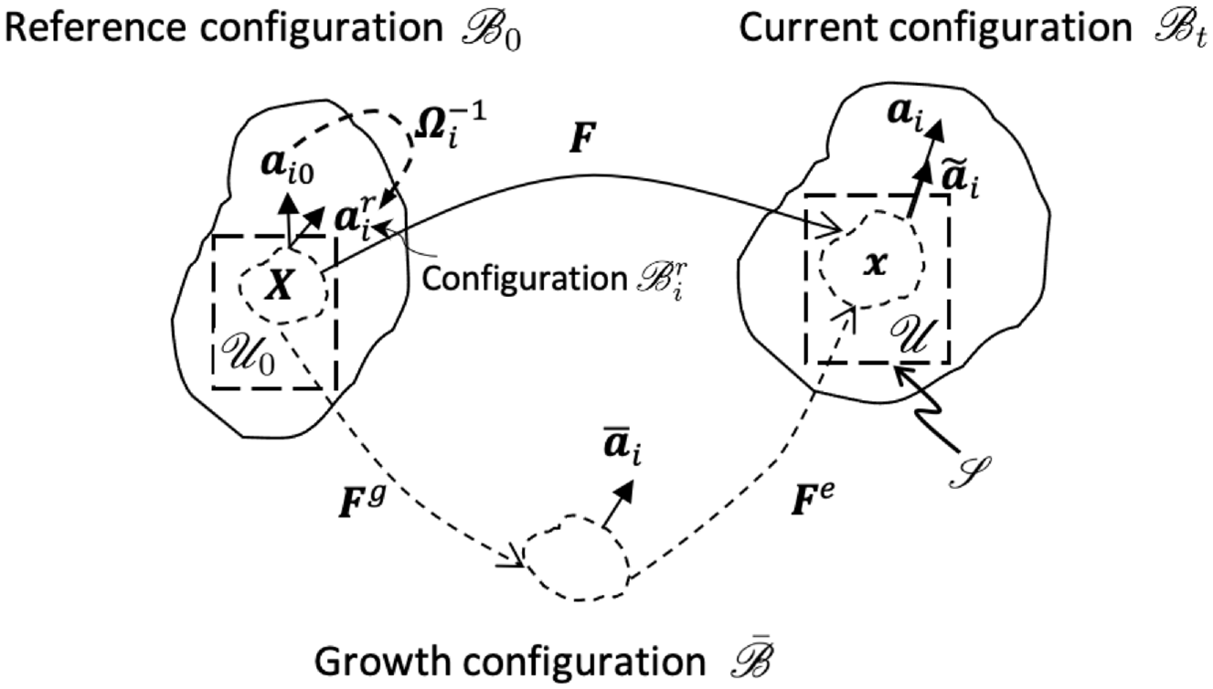
We consider a spatial representative volume (REV) composed of a representative domain of a deformable solid continuum in the current configuration, (see Figure 3). At the current time, , the REV of a spatial point is a geometric domain, , with a closed surface, , embedded into the Euclidean space . Due to growth, this domain represents the material domain of an open system. For an infinitesimal increment of time, a solid phase of this domain may have incremental growth and microstructure remodelling (G & R) imposed upon it. So, it is reasonable to establish an incremental growth theory on . It is assumed that through such an incremental theory, we may trace back to a reference configuration, , at a certain initial time, , with a material point labelled by so that there is a relation, , whereby is the reference geometry domain of and is the mapping to trace back the material point .
Kinematics of modelling: the REV of a spatial point as a geometric domain with a closed surface .
In general, the surface of the REV is not a material surface because of the existence of mass fluxes passing through the surface to supply the new material for growth [49]. In this study, it is assumed that there is no mass flux passing through the surface so that is a material surface. This is consistent with the definition of the first-order kinematical growth [49–52] and the interpretation of the G & R model proposed by Humphrey and Rajagopal [53] that an actual growth process including mass transport may be mathematically modelled as a local mass generation and absorption process. Under such an assumption, the new material deposition and transport in cell wall can be modelled as a local volumetric growth inside the domain matching the local irreversible isochoric expansion for maintaining a certain geometry or structural stability condition, which leads to a non-associated flow rule with the contributions from both expansion and volumetric growth as shown later in section 5.5. Moreover, non-symmetry of the Cauchy stress tensor in an open system [49,50] may be avoided tactically. Hence, growth and remodelling of the cell wall may be expressed in a framework analogous to that of a closed system.
Consequently, the kinematics may be described in a way similar to the conventional continuum theory of a closed system. The mapping is defined as a deformation which maps the reference configuration, , onto the current configuration, , so that the current position of the material point is written as , where is dropped from the expression for conciseness. The deformation gradient is defined as with its Jacobian denoted as .
Let a unit vector, , denotes the initial fibre direction of the family of fibres attached to a solid particle at the material point on . In theory, , the total number of the families of fibres with different directions in the REV, could be any finite number depending on the feature of material, e.g., symmetry. In this study, the fibre may be referred to either the physical CMF or a pure geometrical direction, e.g., the normal direction of the cell wall surface. For clarity, we shall explicit use “CMF” where the fibre refers to physical CMF. Noting that, from the point of view of laminated composite, this study models all CMFs in the REV as a discrete set of finite number families of CMFs with distinguishing directions, which is capable to capture the major features of the cell wall of interest. In reality, either from perspective of single lamina or multiple plies of cell wall, CMFs may have a continuous dispersion of fibre angles, which can be described using a probability density function of a continuous random orientational variable. The reader may refer to the plastic spin theory using the ODF proposed by Dafalias [38], the soft matter model with distributed collagen fibre orientations presented by Gasser et al. [33], and the fibres orientation density distribution for fibrous tissues growth and remodelling by Lanir [27].
The current spatial fibre direction of at the same material point is as follows:
where the deformed fibre and its stretch are described by:
in which “:” denotes the double contraction, “” is the trace operator on , the right Cauchy–Green tensor is defined as:
and are the two structural tensors, and represents a rotation of the fibre due to remodelling. The tensor itself is an orthogonal tensor as the representation of rotation. The superscript stands for the operator of matrix transpose while ⊗ is the tensor product. To differentiate from the fixed fibre direction , a time-dependent fibre direction on is introduced as:
with the corresponding structural tensor, , to represent the evolution of fibre direction with remodelling.
Strictly speaking, we may consider equation (4) as a definition of the remodelling configuration of the family of CMFs, denoted as . is identical to except the fibre direction so that it has the same mapping and the same deformation gradient from to . In other words, if the unit tensor (i.e., , where is the Kronecker delta) is the metric tensor on , the metric tensor on is , which is helpful for clarification of some concepts of the remodelling spin as we may see in the later discussion.
Noting that, to avoid confusion in formulation, the summation rule is not applied to the indexes indicating the families of fibres (e.g., the index “” in equations (1) and (4)) throughout this study.
As the base of kinematical growth modelling, the assumption of the kinematical decomposition of the total deformation gradient,
which was proposed initially for plasticity [54] and then found its place in biomechanics [55], is used in this study, whereby the superscripts “” and “” refer to elastic and growth parts, respectively. Bear in mind that includes the contributions from both the stress-driven isochoric expansion and the matching volumetric growth resulting from material deposition and transport. The decomposition (5) naturally introduces an intermediate configuration, , i.e., the growth configuration generated by , which is a collection of local domains since in general is not a compatible tensorial field. For this reason, as a whole may be considered as a fictitious configuration.
The counterparts of the vector and tensor on , which may be obtained by a pull-back from to , are denoted as:
and , respectively. Noting that the hypothesis of no growth in a CMF direction due to the CMF’s inertia in growth is adopted in this study. As shown in later discussion, Spencer’s deviatoric stress tensor serves as a proper driving force of growth which imposes a certain constraint on so that and the vector is automatically a unit vector on . Hence, and on , on , and on are all treated as the unit vectors.
Equation (6) indicates that the tensor may be interpreted as the deviation of the fibre direction, , from a virtual direction, , complying with the perfectly bonding assumption. By contrast, the elastic deformation of a fibre still obeys the perfectly bonding condition since .
For convenience, the kinematical relations of the different configurations, particles, and fibre directions during a growth process are shown in Figure 3.
2.2. Kinematical relations in rate formats and the growth spin
Aiming at an incremental description of growth, kinematical relations in rate formats are discussed here, which naturally introduces the concept of the growth spin of the wall matrix.
Let be the spatial velocity gradient on , where the symbol of superimposed dot denotes the material time derivative. An additive decomposition of the velocity gradient, which is the rate format of equation (5), may be expressed as:
where elastic and growth parts of are defined as:
respectively, in which the counterpart of on is:
In consistence with equation (9), a pull-back of from to yields:
Furthermore, , , and may be decomposed into symmetric and skew-symmetric parts as:
and
whereby the rate of deformation tensor, , and the material spin tensor, , of the whole continuum of the REV are defined as:
respectively. In a similar way, the spatial elastic and growth rates of deformation may be defined as:
respectively. Moreover, the growth spin, , and rigid body spin, , of the matrix, i.e., crosslink network including the hemicellulose and pectins in the REV, are defined as:
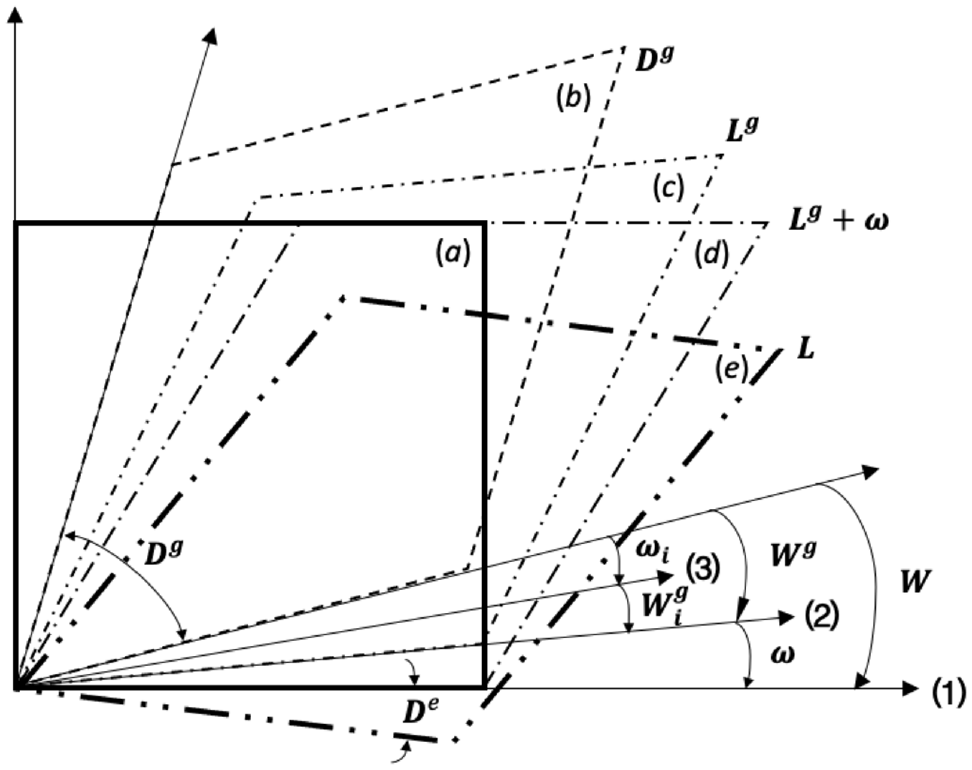
Growth spin and remodelling spin : (i) The reference configuration is mapped in sequence to the configurations , , , and by , , , and , respectively and (ii) The reference fibre direction is mapped to the direction by complying with the perfectly bonding assumption and then re-orientates to the direction by the remodelling .
Correspondingly, pulling and from back to yields:
where we have the relations, and . And the pull-back of from to reads:
Noting that
2.3. Remodelling spin on
Bear in mind that is defined as the growth spin of the wall matrix, with which CMFs convect. We shall separately introduce the spin of CMFs due to the presence of remodelling. To differentiate from , such a spin of CMFs is called the remodelling spin.
For the family of CMFs , an additive decomposition on is introduced as (see Figure 4):
which is in a similar form as equation (12) in Dafalias [56] so that it clearly indicates the connection/analogy between cell wall and crystal plasticity, whereby the remodelling spin, , of the family of CMFs on is defined by a transformation,
in which:
is the corresponding remodelling spin on and its skew-symmetric part is defined as:
In order to interpret the form of equation (21), we may recall the remodelling configuration defined in section 2.1. The remodelling spin , as shown in equation (20), actually is a “velocity gradient” on corresponding to the “deformation gradient,”. As aforementioned, the metric tensor on is . Hence, the operator on is in a form of , which explains equation (21).
Given and , the corresponding constitutive spin, , of the family of CMFs is defined by equation (18) as the difference between of the matrix and of the family of CMFs. may be interpreted as the remodelling of the family of CMFs with respect to of the matrix. Thus is the rate of rotation of the family of CMFs taking into account the convected rotation with the growth spin of the matrix and the remodelling spin of CMFs.
In the specific case that there is no remodelling, i.e., equation (18) indicates that which retains the perfectly bonding assumption for the growth of the whole continuum. Based on the above discussion, of the matrix is a rigid body spin which should be eliminated from the constitutive model of the continuum. Therefore, the objective rate of a tensor, say , associated with the continuum, with respect to , may be defined as:
where the superposed ° follows the notation proposed by Dafalias [48].
In order to define the objective rate of tensors associated with the family of CMFs , we use the general definition of Lie derivative [57–60]:
in which stands for the motion composed of the mapping of the continuum and the remodelling rotation while the subscript “” stands for the velocity field of , and are the corresponding pull-back and push-forward operators, respectively.
For the specification of , let us first consider the motion of the unconstrained structural tensor, , defined in equation (2)1. So that we have the specified pull-back and push-forward as follows:
Substituting equation (24) into equation (23) yields the objective rate of a tensor associated with the family of CMFs, say which is defined on and could be either a geometric or a stress tensor, as:
where the superscript “” stands for the current configuration, and is defined and may be decomposed as:
in which we recognise the remodelling spin and define a symmetric tensor,
Whereby, in consistency with equation (21), the symmetry part of is defined as:
It is understood that in general if . Equation (28) indicates that, given a tensor , may be computed either directly from or from via solving with equations (19) and (21).
With this relationship, the comparison between equations (25) and (22) indicates that:
In the case of no remodelling, we have and . Consequently, equation (32) degenerates to an expression of the continuum.
For further understanding the remodelling spin and the objective rate , let us consider a special case that the structural tensor is assigned to , i.e., . The push-forward in equation (24)2 and the transformation in equation (2)1 indicate that . Hence, , which, using the definition (23), comes to the conclusion:
Equation (33) may be considered as a kinematical remodelling law on based on the motion of .
Since under elastic deformations, the objective rate of the normalised structural tensor:
may provide a more clear and direct description of remodelling.
In this case, the motion may be specified by a mapping derived from equations (1) and (2):
Hence, the specification of the pull-back and push-forward is as follows:
where the superscript “” stands for the unit vector at , and we use the following result:
which is discussed in Appendix 1 (Calculation of ).
The other way to derive equation (37) is to use the relation:
Since , by calculating the trace of equation (25) with replaced by and then exchanging the sequence of trace operator and differentiation operator, we obtain:
It is of interest to observe that there is analogy between the relation, , and the relation, , of Cauchy stress and Kirchhoff stress, where . That is why the objective rates (equations (25) and (41)) (and their relation) show analogies to the objective (e.g., Truesdell) rates of Cauchy stress and Kirchhoff stress (and their relation) [58,59]. This observation may be helpful for the clarification of the objective rates defined here.
Again, we consider a special case that the structural tensor is assigned to , i.e., . Using the same reasoning for deriving equation (33), we may obtain the other kinematical remodelling law on :
Equations (33) and (42) are consistent with the differential geometry concept of the invariance of a tensor field (e.g., or in here) under some transformation, which is expressed by the vanishing of Lie derivative of that tensor field (see Schutz [57], p. 86).
One of the application of equation (42) is to construct a structure-preserving increment of the unit vector :
It is straightforward to prove that:
2.4. Remodelling spins on and
It is interesting to understand the counterparts of the kinematical remodelling law (42) on and , respectively. For this purpose, we use the same pull-back as equation (10) to transform equation (18) from to :
where:
in which is the remodelling spin on .
The objective rates on and associated with the family of CMFs may be derived using the Lie derivative (23) in a process similar to what discussed in section 2.3. Specifically, for the objective rate on , the corresponding motion may be specified by a mapping . Moreover, the objective rate on may be obtained using a motion defined by the mapping in equation (4). However, rather than explicitly using the Lie derivative (23), here we show the other method, which is in a way similar to equation (39), to obtain the objective rates on and through transformations from to and , respectively.
Let us consider a tensor associated with the family of CMFs, say which is defined on and has a relation, , with the aforementioned tensor on . Using equations (8) and (10), this relation has the rate format as:
which, using equations (7) and (8) and some algebra manipulation, may be transformed to:
We may defined an objective rate of , denoted as , via the relation:
in which the superscript “” stands for the growth configuration, . Using this definition and substituting the first relation in equation (26), , into the r.h.s of equation (47), we obtain an expression,
Alternatively, we may substitute the second relation in equation (26), , into the r.h.s of equation (47) and then obtain the other expression of the objective rate,
where, in consistency with equation (45)2 and with the help of the definition (27), we define:
Furthermore, for studying the objective rate on , we consider a tensor associated with the family of CMFs, say which is defined on and has a relation, , with the tensor on .
Substituting the relation, , into equation (25) and going through a process similar to the above discussion from equations (46)–(49) lead to a relation:
where the objective rate of is obtained as:
in which the superscript “” stands for the remodelling configuration. This is consistent with the definition of as the remodelling spin on (see equation (20)).
Similar to on , and are the unit vectors representing the time-dependent fibre directions on and , respectively. Thus, the kinematical remodelling laws in terms of the corresponding geometrical structural tensors, and , are:
respectively, which may be derived either directly from equation (33) with the transformations (48) and (52) or from the Lie derivative (23) with the definition of the push-forwards,
respectively.
Similar to equation (43), equations in (54) give the incremental motion of CMFs. For example, equation (54)2 gives which is the increment of the structural tensor on the configuration (or ) solely due to the remodelling spin .
3. The framework of constitutive model
3.1. Elastic constitutive law and the model of growth and remodelling in general forms
With the kinematics of growth and remodelling defined, we consider the constitutive modelling framework covering elastic responses and growth and remodelling behaviours of the cell wall.
The state variables of the cell wall material may be defined on the current configuration in terms of Cauchy stress, , and a set of hardening variables consisting of (i) a second-order tensor, , and a scalar, , for growth and (ii) a set of second-order tensors, , for the remodelling of each and every family of CMFs .
Accordingly, a set of constitutive equations, which are adopted and extended from the viscoplasticity model of metallic materials proposed by Dafalias [48], fully describe the growth and remodelling behaviours of interest:
1. The tangential elastic relation of the continuum,
2. The coupled irreversible isochoric expansion and volumetric growth of the continuum and the associated hardening behaviour,
and
3. The remodelling of the family of CMFs and the associated hardening behaviour,
The four-order tensor represents the tangent elastic moduli of the stress rate which, via equation (65) below, may be derived from hyperelasticity as shown later in section 5.1.3. The functions , , , , and are the non-negative scalar overstress functions while and are the numbers of the terms of the sequences of the overstress functions for growth and remodelling, respectively. Moreover, , , , , , and define the admissible directions of , , , , , and , respectively. Noting that and are independent from each other. The invariance requirements under the superposed rigid body rotation render all of the tensor and scalar-valued constitutive functions of equations (56)–(59) the isotropic functions of their variables, , , , and .
The objective rate in equations (56) and (58)1 is introduced here based on the postulate that the rates of changes of and are in reference to , instead of [48]. This may become more clear if we re-formulate equations (56) and (58)1 using a rate of change with respect to , i.e., the well-known Jaumann rate. By substituting for according to equation (15) and using equations (14), (15), (22), and (56)–(59), equation (56) may be re-expressed as:
where:
is the Jaumann rate. In the same way, hardening law (58)1 may be re-expressed as:
It is observed that, as the introduction of the growth spin , the growth spin direction, , plays the role of a structural tensor which introduces the additional anisotropic terms into the constitutive model (60) and (62), where the conventional Jaumann rate is used.
Similarly, using elastic Truesdell rate of Cauchy stress tensor [59],
where the elastic tangent moduli for the elastic Truesdell rate is:
in which is defined by [59]. Accordingly, the evolution of in equation (58)1 is re-written as:
The Truesdell rate is useful where hyperelastic formulation is applied since such a formulation naturally leads to a rate format elastic constitutive law using the Truesdell rate.
3.2. Specification of the hardening laws to the growing cell wall
In the continuum modelling of growth and remodelling, hardening laws should be paid significant attention as they may play a unique role to represent the underlying mechanical and non-mechanical mechanisms of living cell walls. This observation was demonstrated by a mechanism-based hardening model proposed for understanding the dynamic regulation of cell wall growth at micromechanical level [17], where growing and non-growing cell walls were clearly differentiated by one single hardening law. Moreover, the mechanism-based hardening model leaded to a scalar phenomenological hardening model (equation (85) in Huang et al. [17]) which may indicate the proper form of specifications of equations (58) and (59)2 for the cell wall growth.
Based on such a consideration, we propose a method for the specification of hardening laws as follows. The hardening model proposed by Dafalias (equation (10) in Dafalias [48]) for viscoplasticity is adopted and modified mathematically for the specification of equations (58) and (59)2, and then the comparison between this type of hardening model and the hardening law proposed in Huang et al. [17] is conducted to show the consistency between them, even though they were proposed originally based on their very own and different mechanisms of the totally different materials. This consistency not only guides and justifies the specification of hardening laws here but also provides the physical interpretation as shown in the following discussion.
In reference to equation (58)1, it is proposed that so that we have . The detail of each term is discussed as follows:
First, for , it is proposed that is proportional to (and depending only on) , i.e.,
with the corresponding overstress function , where is the overstress function of growth as shown in equation (57).
Second, for , with as well, is specified in a coupling form as:
where is a tensorial function of , and is the norm of a tensor (·).
Third, for the remaining term , we set:
as a tensorial function solely in terms of . Accordingly, it is requested that is explicitly independent of strain/stress so that is decoupled from . For this purpose, may be expressed solely as a functional of , i.e., An example of using power law is:
According to equation (71), is consisting of three distinct terms. The strain hardening term, , and the dynamic recovery term, , occur only when (i.e., ), while the static recovery term, , operates always as long as .
If we further specify that, and use the power law (70), equation (71) becomes:
As aforementioned, in order to clarify the role of each term in the r.h.s of equation (73) (or equations (71) and (72)) and justify the specification of the hardening laws (71)–(73), it is helpful to compare equation (73) with the mechanism-induced hardening law of cell wall growth proposed in equation (85) of Huang et al. [17], which is cited here as:
where and are the hardening variable and scalar growth rate, respectively, and and are the two constants. According to the discussion in Huang et al. [17], a comparison between equations (74) and (73) indicates that the first term in the r.h.s of equation (73) (or equations (71) and (72)) represents the strain hardening of the cell wall matrix due to the increase of tension in the crosslink network of the matrix. And the second term represents the effect of softening of the crosslink network due to two contributions: deposition of new load-bearing crosslinks coming in from outside and reconnection of the cut tethers and broken hydrogen bonds inside the cell wall. Hence, the second term features the key regulation mechanisms of growing cell walls as a living material. The third term in the r.h.s of equation (73) (or equations (71) and (72)), which does not have the counterpart in equation (74), may be interpreted as a chemical regulation term which is not explicitly dependent of mechanical regulation as there is no explicit dependency on strain/stress in the expression. Gravitropism provides a typical example demonstrating the coupling between chemical regulation and mechanical regulation of growth [61,62].
Therefore, in the light of equation (74), the specification of hardening laws in equations (71)–(73) can be justified by the physical interpretation. Furthermore, in a form similar to equation (72), equation (59)2 of the hardening of a remodelling process may be specified as:
where the second-order tensor, , is the driving force of remodelling and is the corresponding overstress function. The hardening internal variable, , may be interpreted as a local back stress created by . Noting that the objective rate in equation (75) is the same as the one in the kinematical remodelling law (42). This is based on the consideration that is associated with . More detailed discussion about equation (75) is presented in the later section of a case study.
4. Invariants and spin representation for the growth and remodelling of cell wall
Hitherto, we consider general situations where the number of families of fibres with different direction, , are in theory any finite number. From this section, we shall confine our attention to the specific case that . The reason of this is that cell wall may be considered as a laminated composite with a finite number of layers. And each layer may be considered as a lamina composed of one or two families of fibres. According to composite theory, we could model the material property of a representative layer and then obtain the whole multi-layer composite property using the lay-up and orientation of the layers. Therefore, it is reasonable to consider typical materials of two families of fibres.
4.1. Spencer’s deviatoric stress tensors as the driving forces of growth and remodelling
Let us consider a material with two families of fibres : (i) the two families of fibres could be both of physical CMFs, or (ii) one family is of physical CMFs while another is simply a pure geometric direction (e.g., a director attached to the continuum).
Under the assumption that CMFs are only extensible elastically, it is required that the driving force of growth should vanish in the direction of each family of CMFs [17]. This requirement naturally leads to the application of the so-called Spencer’s deviatoric stress tensor proposed by Spencer [30] and adopted and extended to be applied to cell wall growth modelling by Huang et al. [17,18].
Spencer’s deviatoric (Kirchhoff) stress, , may be derived from an expression,
and its constraints,
Whereby is the Kirchhoff stress while . The index “” refers to the family of fibres as aforementioned. The first constraint in equation (77) makes sure satisfying the isochoric condition while the second constraint eliminates the stress component in both directions of the two families of CMFs. Hence, serves as the proper driving force of the isochoric wall expansion prohibiting inelastic extensions of CMFs.
where is the deviatoric operator on , and the index is the complementary index of an index in the set , i.e., and (numerically ).
For the purpose of growth modelling using finite element method, it is useful to have the counterpart of on where finite element formulation is more convenient in contrast to that on . Pulling from back to by a transformation,
yields the expression of Spencer’s deviatoric PK2 stress, , as:
where is the second Piola–Kirchhoff (PK2) stress on while and are the coefficients to be expressed in terms of variables on .
Noting that we have such a relation between the deviatoric parts of and ,
where and within its r.h.s are the deviatoric and trace operators on , respectively. It is observed that .
Hence, using relation (82), the scalars, and , in equations (78) and (79) may be expressed in terms of the variables on as:
where , in which the weighted structural tensor is defined as:
while is the corresponding weighted vector.
It can be proven that Spencer’s deviatoric PK2 stress satisfies the constraints consistent with equation (77),
where . Furthermore, if the Mandel-stress-style tensors corresponding to and are introduced, respectively, as:
the constraints in equation (86) may be re-expressed as:
Mandel-stress-style tensors play the important role in the constitutive modelling of growth [49] and finite element formulation [59]. We shall see the application of this type of tensors in formulations on in the subsequent discussion.
4.2. Invariants for the model of growth and remodelling
The purpose of this section is to list the invariants which may be potentially used for constructing yield functions of the growth and remodelling of the cell wall. Yield functions should be in terms of the invariants for their objectivity, i.e., invariance under rigid body motion or observer transformation [63].
Since this study involves a large number of tensors, it is unlikely and unnecessary to list the invariants of all of tensors and their combinations. Therefore, we select a typical set of second-order tensors including (i) a stress tensor, (ii) a geometric structural tensor, and (iii) a hardening tensor to demonstrate the forms of invariants. The result presented in this section may be applied to other set of tensors accordingly. For more discussion about the invariants related to Spencer’s deviatoric stress or general theory of the representation of anisotropic invariants, the reader may refers to the publications [30,64–68].
4.2.1. Invariants on t
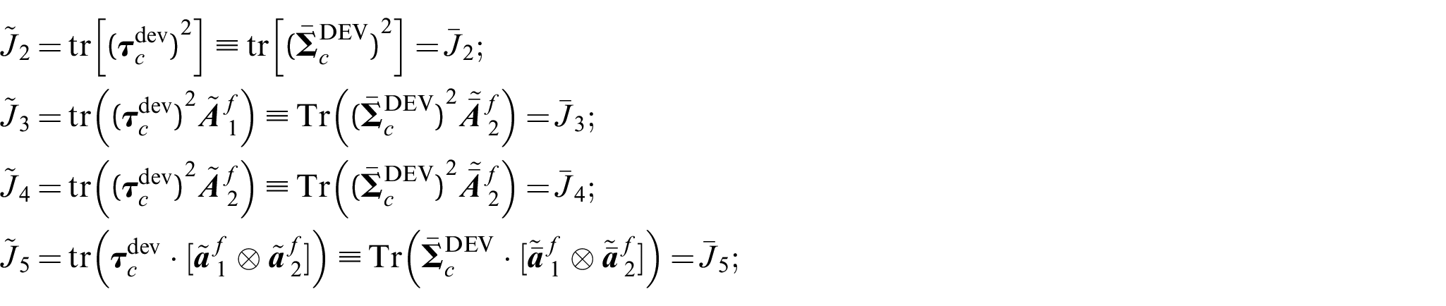
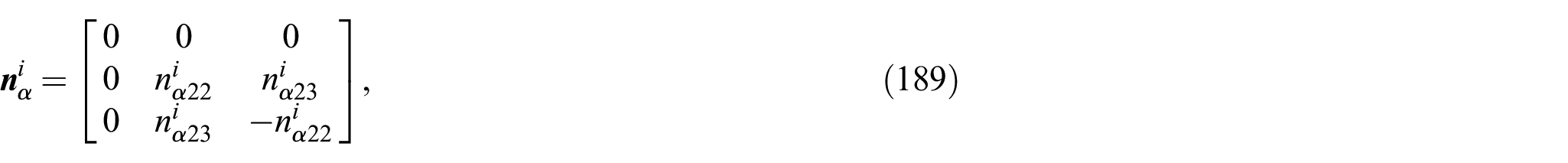
In consistency with the aforementioned set of state variables of the constitutive model, the invariants of the continuum on with two families of fibres may be expressed in terms of Kirchhoff stress , the geometrical structural tensors , and the Spencer-deviatoric-stress-like hardening tensor, , which is introduced in equation (58)1 and here is requested to satisfy the conditions:
where are the structural tensors characterising the hardening tensor so they are similar to, but need not to be identical to, . We take this typical set of second-order tensors, to demonstrate the forms of invariants, which shall be applicable to other set of second-order tensors.
The invariants in terms of , , and are listed as follows:
1.
2.
3.
4.
5.
Alternatively, the invariants may be presented in terms of (and where it is needed), , and as follows:
1.
2.
3.
4.
5.
4.2.2. Invariants on
In a similar way, the invariants may be expressed in terms of variables defined on , which is useful for finite element formulation. For this purpose, in addition to the geometrical structural tensor defined in equation (85) and the Mandel-style stress tensors and defined in equation (87), a Mandel-stress-like hardening tensor, , is introduced here as:
where:
is a PK2-like hardening tensor transformed from by a pull-back.
Thus, the invariants on are expressed in terms of (and where it is needed), , and as follows:
1.
2.
3.
4.
5.
4.3. Spin representation for the model of growth and remodelling
In essence, spins are the second-order skew-symmetric tensors, which is naturally related to the concept of differential forms (see, e.g., p. 104 in Marsden and Hughes [60] or p. 115 in Schutz [57]). According to the definition of differential forms, given two symmetric second-order tensors, say and , we may compute their wedge product,
and conduct the tensor contraction as shown in an index format,
It is straightforward to prove that is a skew-symmetric tensor.
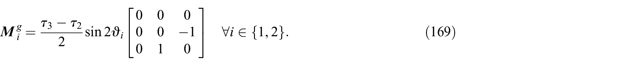
Based on the form in equation (93) and referring to the general format of spin proposed by Dafalias [69], the set of skew-symmetric tensors may be taken as the basis of the representation of the growth spin on is constructed from the set of state variables of the constitutive model, , listed as follows:
Moreover, the corresponding set of tensors on constructed from the set of state variables, is as follows:
The relation between the tensors in the above two sets is the same relation between Kirchhoff stress on and Mandel stress on . To demonstrate this observation, first we show that for the first tensors in both sets, we have:
where we use the definition (87) and a relation, , derived from equations (34) and (85). Second, using equations (87) and (90), it can be proved that for the third tensors in both sets, we have:
The growth spin and remodelling spins may be constructed as linear combinations of skew-symmetric tensors in the forms as shown in this section. We shall discuss the application in section 5.6.
4.4. Yield surfaces
As aforementioned, wall yielding or loosening is the necessary condition of wall expansion under turgor pressure [3,13]. The Lockhart equation indicated the threshold of turgor pressure for cell wall growth [14], which was generalised to the concept of yield surface of growth [15–17]. In consistency with the Lockhart equation, which was cited in Huang et al. [17], the yield surface of wall expansion, , may be defined on in a general form in terms of , , , as:
or equivalently on in terms of , , , as:
where . For the objectivity of a yield surface, the yield surfaces and must be expressed in terms of the invariants as discussed above. Therefore, mathematically, what exactly implies is that and are the identical functions in terms of the invariants which may be expressed in terms of variables on and , respectively. For example, where .
An anisotropic yield surface with isotropic hardening law was reported in the cell wall growth model in Huang et al. [17]. The case study discussed subsequently uses an anisotropic yield surface adopted from the previous studies [17,30] with an isotropic hardening law for the wall growth while using a kinematic hardening law for the remodelling of CMFs. This gives a thorough demonstration of the proposed growth spin theory.
Noting that such a kinematic hardening laws requires a method to compute the objective rate of Spencer’s deviatoric stress tensor (and of ), which we discuss in details in Appendix 1 (The objective rate of Spencer’s deviatoric stress tensor).
5. Case study: cell wall as a cylindrical wall of elastically incompressible material
A cell wall may be simplified as a closed cylindrical wall of elastically incompressible material subjected to an inner (turgor) pressure, (see Figure 5). The assumption of incompressibility is due to the property of space-filling pectins [70]. The general theory about the finite deformation elasticity of cylindrical wall structures may be referred to Ogden [63] while Soldatos [71] provides the extensive discussion about the mass growth of axisymmetric fibre-reinforced tubes.
The model of cell wall as a cylindrical wall with two mechanically equivalent families of CMFs. The fibre angle represents the CMFs’ temporal–spatial distribution.
In such an idealised geometry model, cell wall growth may include the expansive growth on the cylindrical side surface and tip growth on two caps of the closed wall. As the interest of this study is on the cell wall elongation in the longitudinal direction by expansive growth, the effect of tip growth can be ignored when compared to the wall elongation according to the experimental observation [9,35] and the theoretical analysis [15]. Therefore, the model may be further simplified to be an open cylindrical wall subjected to (i) the inner (turgor) pressure on the wall surface and (ii) the equivalent loads, , on two end sections of the open wall obtained by lumping the turgor pressure applied on the cap of the closed wall and then transferring to the end section of the open wall (see Figure 5).
The wall is considered as a laminated composite with a finite number of layers. From the point of view of composite lay-up, it is assumed that the wall has a balanced lay-up of the layers (say, [−45/45]) which, however, is not necessary to be symmetrical with respect to the centroid of the composite shape. In other words, the lay-up on the two sides of the wall cross-section centroid need not to be symmetrical as indicated in the literature [2,72]. Thus, we may assume that (i) each layer consists of two families of CMFs which are mechanically equivalent locally (so that a double helical distribution globally) and (ii) the whole structure is axisymmetric (see Figure 5). It is also assumed that the lay-up throughout the wall, i.e., the distribution of the fibre angles of CMFs along the wall thickness direction, is known. As reported in the literature [2,72], the CMFs in the innermost layer of the wall, which are the latest deposited by wall growth, are aligned in the circumferential direction of the wall. From the innermost surface to the outermost surface along the wall thickness direction, the distribution of the fibre directions may sequentially change from the circumferential direction towards a direction closer to the longitudinal direction of the wall, which is an interesting non-symmetrical lay-up from the points of view of growth modelling and mechanical design.
5.1. Governing equations
5.1.1. Kinematical equations
In the reference configuration , the cylindrical geometry of the wall is defined in terms of the cylindrical coordinates by:
where and are the inner and outer radii, respectively, of the wall on and is its length.
In terms of the spatial coordinate system, , the geometry of the wall on the current configuration experiencing growth and elastic deformation is given by (see Figure 5):
where is an unknown function that depends on both the growth and the elastic deformation, and is the stretch in the longitudinal direction at the current time . Thus, we have:
where the current inner and outer radii, and , of the wall are unknown unless specified as part of boundary conditions.
Let and be the orthonormal bases of the cylindrical coordinate systems on and , respectively, where are the unit vectors in the longitudinal principal direction of the wall. Hence, equation (98) may be expressed in a vector format as:
where is the projection of a vector from to . The deformation gradient is then obtained as:
in which is an unit two-point tensor. From the expression, , the derivative in the r.h.s of equation (100) can be worked out as:
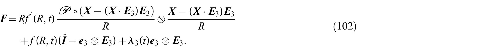
where a prime indicates the derivative with respect to . So that the expression of in equation (100) becomes:
Thus, is symmetric and its principal axes coincide with the cylindrical axes. The corresponding principal stretches of , , , and , are then simply read off as:
5.1.2. Equilibrium equations
The equilibrium equation on without body force is:
where ∇ is the gradient operator on . Similar to equation (102), the Cauchy stress in the coordinate system may be expressed as:
where are the principal stresses of . The equilibrium equation in this case reads:
5.1.3. Elastic constitutive law of the growing cell wall
Let and be the free energy per unit mass on the configuration and the free energy per unit fixed volume on , respectively. We have the relation:
where is the mass density on while is the mass density on . The mass balance is simply expressed as:
where and are the mass sources per unit volume on and , respectively, representing the effects of material deposition, transport, and integration, whereby mass fluxes are not considered explicitly for the reasons mentioned in section 2.1. Equation (108)1 indicates that the density within changes with growth, just as the fibre direction on changes with remodelling.
The assumption of constant density on , which is one of the key features of kinematical growth model [49], may be expressed as:
Equations (109) and (110) indicate that (i) the mass source purely contributes to the volumetric part of growth, and (ii) the change of is purely elastic.
Based on this observation, a specification of may be introduced as:
where , and is the free energy density per unit volume on the configuration so that . Here, we are concerned only with the volumetric part of growth (110) and the remodelling due to the additional fibre rotation , so that the material response characterised by is independent of . Moreover, the implications of objectivity require that depends on through the right Cauchy–Green tensor and the free energy function should be in terms of the invariants of a set of tensors, [17,33].
In the case of interest that the elastic response of the material is incompressible, i.e., , a Lagrange multiplier, , is introduced to replace by . Then, it can be deduced in a standard way (see, e.g., Ogden [63]) that the elastic constitutive equation of such a material is in a form as:
The corresponding tangent moduli in equation (64) may be computed from the transformation,
where is the elastic tangent moduli on . More details of the expressions of Cauchy stress and tangent moduli of the cell wall model may be referred to Huang et al. [17], which was adopted from Gasser et al. [33].
5.2. Elastic solution of Cauchy stress
Let us consider part of the wall between radii and in (see Figure 5). The volume of this part is:
Due to the elastic incompressibility, the elastic response from to is volume-preserving, and the corresponding material volume on should be equal to the one in equation (114). However, since the deformation gradient is in general incompatible and the configuration is only a collection of infinitesimal domains, the corresponding volume on cannot be calculated with a similar formula as equation (114). We denote this volume by , and calculate it by a push-forward from to with the Jacobian :
where:
The elastic incompressibility indicates that the two volumes in equations (114) and (115) are equal,
and hence,
The stretch is then obtained as:
Consequently, the relations in equation (103) indicate that:
It is observed that, (or equivalently the length ) and the inner radius of the wall, , in equations (118) and (119), are yet unknown when is known once the growth law is specified. To determine and , we need to obtain an expression of Cauchy stress in terms of the elastic principle stretches and then to solve the problem using the equilibrium equation and boundary conditions.
In this case, is diagonal with the principal stretches denoted by , , and . The free energy depends only on the stretch , and we represent this dependence as:
The reason of choosing and as the major variables is that the major driving force of growth is considered in an in-plane direction.
must satisfy the traction boundary conditions: (1) on the inner surface, and (2) on the outer surface, . By integrating equation (124) with respect to from to and using the two-point traction boundary conditions of , we obtain:
Hence, in the integral (125) is determined by and if the growth is specified.
In addition to equation (125), we need the equilibrium condition in (longitudinal) direction to completely determine and . For this purpose, integrating equation (124) from to yields:
Hence, the resultant force, , on the end section of the open wall in the longitudinal direction, is obtained by integrating over the end section area as:
In addition, given the turgor pressure , the total force applying on the end cap of the closed wall is , which is equivalent to the resultant force in equation (129) (refer to Figure 5):
Given the growth (i.e., ), the equilibrium conditions (125) and (129) together with equations (126) and (130) are sufficient to determine and , which completely solves the elastic deformation of the wall. Consequently, equations (127), (128), and (122), which is re-written in a form as:
provide the principal stresses of in terms of and .
5.3. Specification of the expressions of τdev
With (and then ) obtained, Spencer’s deviatoric stress tensor can be calculated according to equations (76), (78), and (79).
As aforementioned, it is assumed that each layer of the wall has two families of CMFs which are mechanically equivalent. This means the driving force of growth of such a layer as a continuum should vanish in both directions of the two families of CMFs due to the inertia of CMFs in growth. However, each family has its own remodelling behaviour depending on its fibre direction and the axis of re-orientation. The driving force of the remodelling should vanish in these two directions as well since any force in these two directions does not contribute to the re-orientation of this family of CMFs and should be subtracted from the total stress.
Therefore, we consider two specifications of the expression of : one with two physically equivalent families of CMFs, the other with one family of CMFs and one pure geometry direction (i.e., the axis of re-orientation). The former is for the modelling of the growth of the wall as a continuum, and the latter is for the modelling of the remodelling of each and every family of CMFs. We discuss the two specifications in details separately.
5.3.1. Specification 1: two mechanically equivalent families of CMFs for the growth of the cell wall
Let us write the radial axis of the wall as and the circumferential axis as , where × is the cross product of vectors. Since the basis of a local coordinate system, , is identical to the principal directions of stress, may be expressed in a diagonal form in this local coordinate system.
Using the local coordinate system , the two families of CMFs of the representative layer are represented by two unit vectors:
where is the angle of family of CMFs on the plane (i.e., the plane expanded by and ) measured from the circumferential axis towards the longitudinal axis around the axis .
The two mechanically equivalent families of CMFs may be specified using a single specific angle ,
Let us assign the values of the two specific vectors to the general unit vectors in equation (1),
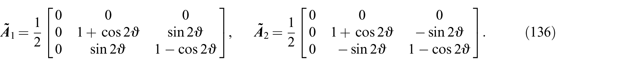
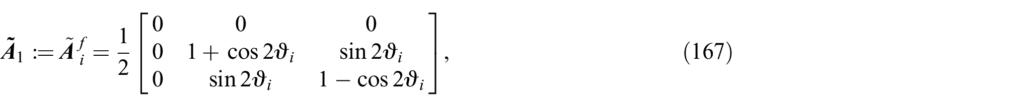
which characterise Spencer’s deviatoric stress in equation (76) via the structural tensor in equation (34). Consequently, the components of the structural tensor are obtained as:
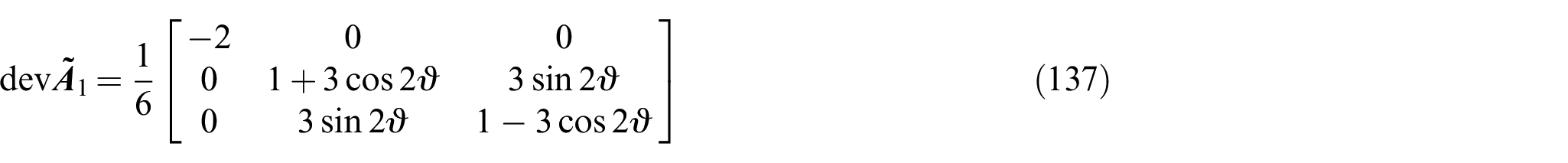
The corresponding deviatoric tensors are:
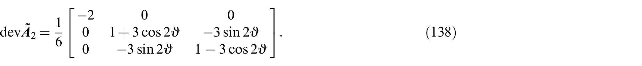
and
Substituting equation (136) into equation (76) yields a specification of for the continuum (i.e., matrix and CMFs) denoted as:
where the subscript “” stands for the continuum, and the diagonal components are:
Substituting equations (141) and (142) into equation (140) leads to the expression of the diagonal components (no summation of the index below):
where the coefficients, , are:
in which:
Equation (143) shows that, using the constitutive equations (122) and (123), the components of may be expressed as the functions of and only since the Lagrangian multiplier is eliminated automatically from equation (143).
in equation (139) is in a form as the direct driving force of wall expansion. As examples, the expressions of in two cases are shown as follows:
Case 1:
Case 2:
Bear in mind that wall expansion must be associated with volumetric growth to maintain wall thickness and strength. However, itself is a traceless deviatoric tensor. Thus, although is assumed as the driving force of growth, a role similar to the deviatoric stress in plasticity, the matching volumetric growth need to be represented by a non-traceless tensor, which is shown in the subsequent discussion about the flow rule of growth.
5.3.2. Specification 2: one family of CMFs and one pure geometrical direction for the remodelling of individual family of CMFs
Here, we consider the remodelling of the family, i.e., one of the two families, of CMFs of a representative layer of the cell wall. Thus, different from equation (135), the two unit vectors, and , are assigned as:
where represents the family of CMFs while is a pure geometrical direction aligning with the radial direction to represent the re-orientation direction. Consequently, the structural tensors in equation (76) for defining Spencer’s deviatoric stress are obtained as:
Substituting equations (145) and (148)–(150) into equation (76) yields the specification of Spencer’s deviatoric stress tensor for the family of CMFs, denoted as:
which indicates that may be derived from two vectors, and , as follows:
is assumed as the driving force of the remodelling of the family of CMFs of the representative layer.
5.4. Yield surface of growth
As aforementioned, cell wall growth is composed of two parts (i) a directly stress-driven irreversible isochoric in-plane expansion and (ii) the out-of-plane volumetric growth by material deposition and transport (see Figure 2(a)). Based on the biological evidences and postulates about wall yielding/loosening [3,13] and mechanics understandings, it is considered that the expansion plays the leading role in wall growth while material deposition and transport are matching the expansion accordingly for maintaining the stability of the wall. Therefore, it is reasonable to assume that a yield surface of wall growth only needs to explicitly account for the yielding condition of the wall expansion. The volumetric growth by material deposition and transport does not affect the yielding condition explicitly but may be taken into account in the flow rule. Under such an assumption, the yield surface of cell wall growth is merely the yielding condition of the stress-driven irreversible isochoric expansion of the wall, which obviously links to von Mises condition in plasticity using a deviatoric stress.
Therefore, it is assumed that the wall growth is driven by the tensor specified in equation (139) and the growth model of the continuum may be formulated using a set of state variables, in which are specified according to equation (135), and is a scalar hardening variable. The yield surface, introduced in equation (96), with isotropic hardening, is proposed as:
where the yield function, on , and its counterpart, on , may be specified, respectively, by adopting the anisotropic yield functions proposed in the previous studies [17,30] as:
in which, similar to equation (87)2, a Mandel-stress-style tensor is defined as:
the weighted structural tensor is defined in a way similar to equation (85),
while , the invariants are referring to the lists in section 4.2 with replaced by respectively, as:
the scalars, , , and , are the yield parameters with the dimension of stress, and the hardening variable is governed by the evolution law (58)2 in a general form and may be specified in a form as equation (73).
Noting that yielding and softening of the growing cell wall have their own biological mechanisms. The yielding is due to the proactive loosening of cell wall crosslinks to enable growth while the softening is part of the dynamic regulation of the cell wall to balance the growth and strength [2,3].
5.5. Flow rules of growth on t and
Let us consider the growth law in equation (57), and , on . In consistency with the yield surface in equation (154), the overstress function may be defined as:
where <*> are the Macaulay brackets.
As aforementioned, Spencer’s deviatoric stress tensor in equation (139) is assumed as the driving force of the wall growth, but its traceless feature indicates that the associated volumetric growth must be represented by other non-traceless tensors. Thus, taking into account the axisymmetric feature, the flow directions of the growth are supposed as:
where the two parts of are:
Equation (159)1 may be considered as a non-associated flow rule on . It may be interpreted that represents the direction of the stress-driven wall expansion while represents the direction of the matching volumetric growth resulting from the new material deposition and transport (Figure 2(a)). Noting that and , which mean (i) the directly stress-driven wall expansion direction is isochoric so it tends to reduce the wall thickness (and strength) during expansion and (ii) the matching volumetric growth is supplied by the new material deposition and transport in the wall thickness direction for keeping a constant wall thickness on (see Figure 2). This is how the cell wall growth differs from the current engineering AM: deposition and transport of new material to maintain the in-plane wall expansion rather than to create an out-of-plane extrusion.
Moreover, we have the pull-back formulae of (i) rate of deformation, , and (ii) spins,
which are consistent with equation (45). Thus, it is straightforward to obtain the counterpart of the growth law (57) on as:
where the growth directions on are:
As the counterpart of equation (159), the specification of the growth directions on is calculated from equation (163) as:
Noting that the r.h.s of equation (164)1 is an expression in terms of the variables on . To obtain the alternative expression in terms of the variables on , the two equations in the growth law (57) are summed up as , which is then pulled back to as:
using the relation, . Substituting the specification (159) into equation (165) yields:
where we use the definition of the Mandel-stress-style tensor in equation (156). From the point of view of the conventional continuum, equation (166) is a non-associated flow rule on .
5.6. Flow rules of remodelling on t and
Hitherto, we complete the growth model of the continuum with isotropic hardening using the set of specified state variables, accounting for the two families of CMFs in one layer. For modelling the remodelling of individual family of CMFs in the same layer with kinematic hardening, we use a set of specified state variables of the family of CMFs, where is defined in equation (151), are specified by equation (144), and is a second-order hardening tensor associated with the family of CMFs which is defined later. Thus, we shall be able to formulate the remodelling of each and every family of CMFs using the invariants and spin representation presented in section 4.2 and 4.3 with replaced by
We consider the remodelling law in equation (59)1, , of the family of CMFs. The overstress function is discussed later in section 5.7. Based on the discussion of the representation of spins in section 4.3, here we show two different formulations to construct the flow direction of remodelling.
5.6.1. Flow direction of remodelling on t: formulation 1
In this formulation, Spencer’s deviatoric stress tensor, , and the associated geometrical structural tensor, , of the family of CMFs, which is assigned to in equation (145)1 as:
are used to construct in a form referring to equation (94) as:
5.6.2. Flow direction of remodelling on t: formulation 2
Different from the formulation (168), in this formulation, Spencer’s deviatoric stress tensor, , and the stress-like hardening tensor, , introduced in equation (59)2 for the family of CMFs, are used to construct referring to equation (95) as:
where, being consistent with equation (89) and similar to , the hardening tensor satisfies the constraints,
in which are the structural tensors characterising the hardening tensor . Noting that and are characterised by the structural tensors and , respectively. It may be interpreted that is the background geometrical structural tensor associated with the hardening state of the matrix resulting from the remodelling of the family of CMFs characterised by the state of . Thus, need not to be identical to .
For clarity, let us construct explicitly in a way analogous to that of . Similar to equation (145)1, may be expressed as:
where , analogous to , is an in-plane angle on the plane. Then, analogous to equation (145), two structural tensors, in which the superscript ‘’ stands for the hardening variable, are proposed as:
By introduction of a so-called back stress, , the tensor may be expressed in a form analogous to in equation (76):
The comparison between equations (169) and (177) indicates that the flow directions of remodelling may be expressed in a united form as:
where the function has the expression,
for formulation 1, or,
for formulation 2. This completes the formulation of the flow direction of remodelling on .
5.6.3. Flow direction of remodelling on : formulations 1 and 2
Regarding the yield function in equation (155) and the growth flow direction in equation (166), it is interesting to formulate the counterparts of equations (168) and (170) on using Mandel-stress-style tensors. This may be obtained using a pull-back transformation similar to equation (163)2,
where is the flow direction of remodelling on .
First, a Mandel-stress-style tensor corresponding to is defined as:
Second, similar to equations (90) and (91), two hardening tensors of remodelling are introduced as:
and
Again, it may be interpreted that is a hardening tensor analogous to the PK2 stress tensor while is a Mandel-stress-like hardening tensor on .
Consequently, the formula (170) of the formulation 2 on may be pulled back to using equations (181)–(183) as:
where the operator, , is defined in the same format as in equation (17). As expected, the flow direction is expressed in terms of the Mandel-stress-style tensors, and .
In a similar way, the pull-back of equation (168) of the formulation 1 yields:
5.7. Hardening law of remodelling
Different from the isotropic hardening law of growth in equation (158), a kinematic hardening law is assumed for the remodelling. Hence, the evolution of the hardening tensor , which is proposed in a general form of equation (59)2, may be specified in a form consistent with equation (75) as,
where in equation (75) is replaced by according to the features of shown in equation (171), so that the objective rate is structure-preserving.
The driving force in equation (187) is specified in a form similar to that of the theory [44,58],
With obtained, the overstress function in the hardening law (187) (and in the flow rule (59)1) may be defined as:
where is a remodelling parameter. Equation (192) implies a remodelling of CMFs not explicitly depending on the wall expansion. Alternatively, equation (192) may be modified as by multiplying the overstress function of the wall expansion, , so that the remodelling is explicitly associated with the wall expansion.
Hitherto, the objective rate of is determined from the hardening law (187). To calculate the material time derivative, , for a complete update of at time , we refer to equation (214) in Appendix 1 (The objective rate of Spencer’s deviatoric stress tensor) and propose that the objective rate is related with the material time derivative in such a form,
where may be expressed in a format analogous to either equation (223) or equation (215). As mentioned in Appendix 1 (The objective rate of Spencer’s deviatoric stress tensor), for analytical analysis, it is more convenient to use equation (215). Therefore, referring to the definition of in equation (174), we write the general form of as follows:
where, analogous to in equation (217), may be calculated by:
in which, analogous to equation (216), the increment of is:
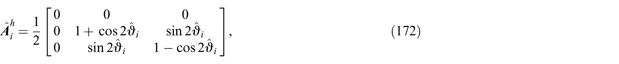
According to the analogies between and the specification of the components of in the r.h.s of equation (194) is obtained by a direct analogy with equation (151) as:
For the remaining part in the r.h.s of equation (194), we first calculate the increment, , in the last term of r.h.s in a way analogous to equation (218) as:
Second, the coefficients, , also in the last term of r.h.s are calculated as the analogies to equations (149) and (150),
Third, we calculate the second term in the r.h.s of equation (194),
and part of the expression inside the third term,
which gives the whole third term in the r.h.s of equation (194),
Noting that equation (205) includes a set of two independent scalar equations sufficient to compute the evolution of the two independent scalar variables, (or ) and , which gives the evolution of the tensor as shown in equation (175).
6. Conclusion
The recent advances in cell wall bring the researchers closer to meeting two grand challenges in this field: (i) to connect cell wall structure to mechanics at the molecular and cellular scales and (ii) to connect cell wall structure to cell growth by identifying the molecular sites of wall loosening and the molecular movements of wall polymers as the cell wall surface enlarges [5]. In order to reflect those advances on continuum theory and to address the challenges from the point of view of continuum mechanics, this study proposes the concept of growth spin and the corresponding model of growth and remodelling of cell wall.
First, the model relaxes the perfectly bonding assumption, which has been widely used in both elastic [33] and inelastic [30] fibre-reinforced material models including cell wall growth models [17,73] with inspiration from Spencer’s work [30,64], so that the continuum model may accommodate the new observation and concepts about cell wall structure at nano-/micro-scale, especially the emerging concept that CMFs make a load-bearing network via close physical contacts rather than a tethered network of CMFs.
Second, it is demonstrated that in the proposed model, the three major components—i.e., CMFs, hemicellulose, and pectins—may have their own growth/remodelling spins, just similar to the plastic spins [38,48,56,69,74] of the slip/twining systems in crystal plasticity, which renders a platform of formulation not only for the antisymmetric part of growth deformation gradient (a term missing from most of the existing kinematical growth models) but also for the remodelling of the individual family of CMFs. This feature provides the more sophisticated and flexible kinematical description of cell wall aiming at quantitatively modelling the postulates of (i) the selective control of CMFs and (ii) flexible means to modulate the directionality of cell growth [5,75].
Third, the corresponding isotropic and kinematic hardening laws are proposed for growth and remodelling, respectively, which further shows the potential of the present model to capture the selective control and flexible regulation of the directionality of cell growth. In addition to generalising the strain-induced scalar hardening law reported in Huang et al. [17] into a tensorial format, a hardening term not explicitly depending on strain is introduced to account for chemical regulation. Together, the proposed hardening model provides a new modelling framework for addressing one of the key questions of cell wall growth: the balance between hardening and softening of the wall material for a dynamical control of growth while maintaining the material strength.
Fourth, this study thoroughly demonstrates the application of Spencer’s deviatoric stress tensors for the modelling of cell wall growth and remodelling. In addition to showing the role of Spencer’s deviatoric stress tensors in the yield surfaces and flow rules, the kinematic hardening law of remodelling shows the calculation and application of the objective rate of Spencer’s deviatoric stress tensor.
Fifth, to the best of the author’s knowledge, unlike the macroscopic plasticity theory which has the micro-structural interpretation using crystal plasticity theory, the kinematical growth of soft matter does not have such a micro-structural counterpart. This caused the difficulty in the interpretation of underlining mechanisms and may be one of the reasons that the growth configuration was considered as a “fictitious” configuration [41]. Based on the recent advances on the nano-/micro-scale mechanics of cell wall, this study may shed a new light into the micro-structural interpretation of the kinematical growth.
In summary, the growth spin model suggests a new framework of constitutive modelling for reflecting the recent advances in the research of cell wall growth and addressing some long-term challenges, especially the integration of the components and the mechanisms to maintain the integrity during growth, from the point of view of continuum theory. The formulation in this study is conducted on both the current configuration and intermediate (growth) configuration, which could be applied to finite element formation in future work.
Footnotes
Appendix 1
Acknowledgements
The author is deeply grateful for the reviewers’ comments which are greatly helpful for improving the clarity and presentation.
Author’s note
This paper is dedicated to the memory of Professor Anthony J. M. Spencer FRS.
Funding
The author(s) disclosed receipt of the following financial support for the research, authorship, and/or publication of this article: The author acknowledges the partial support of MRC (UK) grant no.11603.
ORCID iD
Ruoyu Huang
References
1.
BaskinTI. Anisotropic expansion of the plant cell wall. Annu Rev Cell Dev Biol2005; 21: 203–222.
2.
CosgroveDJ. Growth of the plant cell wall. Nat Rev Mol Cell Biol2005; 6(11): 850–861.
3.
SchopferP. Biomechanics of plant growth. Am J Bot2006; 93: 1415–1425.
CosgroveDJ. Nanoscale structure, mechanics and growth of epidermal cell walls. Curr Opin Plant Biol2018; 46: 77–86.
6.
GeitmannAGrilJ. (eds) Plant biomechanics: From structure to function at multiple scales. New York: Springer, 2018.
7.
IwamotoSKaiW IsogaiAIwataT. Elastic modulus of single cellulose microfibrils from tunicate measured by atomic force microscopy. Biomacromolecules2009; 10: 2571–2576.
8.
MargaFGrandboisMCosgroveDJ, et al. Cell wall extension results in the coordinate separation of parallel microfibrils: evidence from scanning electron microscopy and atomic force microscopy. Plant J2005; 43: 181–190.
9.
ProseusTEBoyerJS. Identifying cytoplasmic input to the cell wall of growing Chara coralline. J Exp Bot2006; 57: 3231–3242.
10.
ProseusTEBoyerJS. Tension required for pectate chemistry to control growth in Chara coralline. J Exp Bot2007; 58: 4283–4292.
11.
CosgroveDJ. How do plant cell walls extend?Plant Physiol1993; 102: 1–6.
12.
CosgroveDJ. Wall extensibility: its nature, measurement and relationship to plant cell growth. New Phytol1993; 124: 1–23.
LockhartJA. An analysis of irreversible plant cell elongation. J Theor Biol1965; 8: 264–275.
15.
BoudaoudA. Growth of walled cells: from shells to vesicles. Phys Rev Lett2003; 91: 018104.
16.
DumaisJShawSLSteeleCR, et al. An anisotropic-viscoplastic model of plant cell morphogenesis by tip growth. Int J Dev Biol2006; 50: 209–222.
17.
HuangRBeckerAAJonesIA. Modelling cell wall growth using a fibre-reinforced hyperelastic-viscoplastic constitutive law. J Mech Phys Solids2012; 60: 750–783.
18.
HuangRBeckerAAJonesIA. A finite strain fibre-reinforced viscoelasto-viscoplastic model of plant cell wall growth. J Eng Math2015; 95: 121–154.
19.
YanagisawaMDesyatovaABeltetonS, et al. Patterning mechanisms of cytoskeletal and cell wall systems during leaf trichome morphogenesis. Nat Plants2015; 1: 15014.
20.
YangHWattsHDGibilterraV, et al. Quantum calculations on plant cell wall component interactions. Int Sci: Comput Life Sci2019; 11(3): 485–495.
21.
YeDKiemleSNRongpipiS, et al. Resonant soft X-ray scattering reveals cellulose microfibril spacing in plant primary cell walls. Sci Rep2018; 8(1): 1–13.
22.
JensenOEFozardJA. Multiscale models in the biomechanics of plant growth. J Physiol2015; 30: 159–166.
23.
OrtegaJKE. Dimensionless number is central to stress relaxation and expansive growth of the cell wall. Sci Rep2017; 7: 3016.
24.
ChakrabortyJLuoJDysonRJ. Lockhart with a twist: modelling cellulose microfibril deposition and reorientation reveals twisting plant cell growth mechanisms. J Theor Biol2021; 525: 110736.
25.
TaberLA. Biomechanics of growth, remodeling, and morphogenesis. Appl Mech Rev (ASME)1995; 48: 487–545.
26.
TaberLA. Towards a unified theory for morphomechanics. Phil Trans R Soc A2009; 367: 3555–3583.
GorielyA. The mathematics and mechanics of biological growth. New York: Springer, 2017.
29.
CosgroveDJ. Re-constructing our models of cellulose and primary cell wall assembly. Curr Opin Plant Biol2014; 22: 122–131.
30.
SpencerAJM. A theory of viscoplasticity for fabric-reinforced composites. J Mech Phys Solids2001; 49(11): 2667–2687.
31.
CosgroveDJ. Plant cell wall extensibility: connecting plant cell growth with cell wall structure, mechanics, and the action of wall-modifying enzymes. J Exp Bot2016; 67(2): 63–476.
32.
ZhangTTangHVavylonisD, et al. Disentangling loosening from softening: insights into primary cell wall structure. Plant J2019; 100(6): 1101–1117.
33.
GasserTCOgdenRWHolzapfelGA. Hyperelastic modelling of arterial layers with distributed collagen fibre orientations. J R Soc Interface2006; 3: 15–35.
34.
MenzelA. A fibre reorientation model for orthotropic multiplicative growth. Biomech Model Mechanobiol2007; 6: 303–320.
35.
ProseusTEOrtegaJKEBoyerJS. Separating growth from elastic deformation during cell enlargement. Plant Physiol1999; 119: 775–784.
36.
ProseusTEZhuGLBoyerJS. Turgor, temperature and the growth of plant cells using Chara corallina as a model system. J Exp Bot2000; 51: 1481–1494.
37.
TorquatoS. Random heterogeneous materials: Microstructure and macroscopic properties. New York: Springer-Verlag, 2002.
38.
DafaliasYF. Orientation distribution function in non-affine rotations. J Mech Phys Solids2001; 49: 2493–2516.
39.
ManiSCosgroveDJVothGA. Anisotropic motions of fibrils dictated by their orientations in the lamella: a coarse-grained model of a plant cell wall. J Phys Chem B2020; 124(17): 3527–3539.
40.
ZhangYYuJWangX, et al. Molecular insights into the complex mechanics of plant epidermal cell walls. Science2021; 372(6543): 706–711.
41.
HuangROgdenRWPentaR. Mathematical modelling of residual-stress based volumetric growth in soft matter. J Elast2021; 145: 223–241.
42.
HavnerKS. Finite plastic deformation of crystalline solids. Cambridge: Cambridge University Press, 1992.
43.
AnandLKothariM. A computational procedure for rate-independent crystal plasticity. J Mech Phys Solids1996; 44: 525–558.
44.
Nemat-NasserS. Plasticity: A treatise on finite deformation of heterogeneous inelastic materials. Cambridge: Cambridge University Press, 2004.
45.
SpencerAJMSoldatosKP. Finite deformations of fibre-reinforced elastic solids with fibre bending stiffness. Int J Non-linear Mech2007; 42(2): 355–368.
46.
SteigmannDJ. Theory of elastic solids reinforced with fibers resistant to extension, flexure and twist. Int J Non-Linear Mech2012; 47: 734–742.
47.
SoldatosKPShariffMHBMMerodioJ. On the constitution of polar fiber-reinforced materials. Mech Adv Mater Struct2021; 28(21): 2255–2266.
48.
DafaliasYF. The plastic spin in viscoplasticity. Int J Solids Struct1990; 26(2): 149–163.
49.
EpsteinMMauginGA. Thermomechanics of volumetric growth in uniform bodies. Int J Plasticity2000; 16: 951–978.
50.
KuhlESteinmannP. Mass and volume specific views on thermodynamics for open systems. Proc R Soc London2003; 459(2038): 2547–2568.
51.
MauginGA. On inhomogeneity, growth, ageing and the dynamics of materials. J Mech Mater Struct2009; 4: 731–741.
52.
SoldatosKP. Modelling framework for mass-growth. Mech Res Commun2013; 50: 50–57.
53.
HumphreyJDRajagopalKR. A constrained mixture model for growth and remodeling of soft tissues. Math Mod Meth Appl Sci2002; 12: 407–430.
DafaliasYF. Plastic spin: necessity or redundancy?Int J Plasticity1998; 14(9): 909–931.
57.
SchutzB. Geometrical methods of mathematical physics. Cambridge: Cambridge University Press, 1980.
58.
SimoJCHughesTJR. Computational inelasticity. New York: Springer, 1998.
59.
BelytschkoTLiuWKMoranB. Nonlinear finite elements for continua and structures. Chichester: John Wiley & Sons, 2001.
60.
MarsdenJEHughesTJR. Mathematical foundation of elasticity. New York: Dover, 1994.
61.
SwarupRKramerEMPerryP, et al. Root gravitropism requires lateral root cap and epidermal cells for transport and response to a mobile auxin signal. Nat Cell Biol2005; 7: 1057–1065.
62.
BandLRWellsDMLarrieuA, et al. Root gravitropism is regulated by a transient lateral auxin gradient controlled by a tipping-point mechanism. Proc Natl Acad Sci USA2012; 109(12): 4668–4673.
63.
OgdenRW. Non-linear elastic deformations. Chichester: John Wiley & Sons, 1984.
64.
SpencerAJM. Deformations of fibre-reinforced materials. London: Oxford University Press, 1972.
65.
WangCC. On representations for isotropic functions, part I. Arch Rational Mech Anal1969; 33: 249–267.
66.
WangCC. On representations for isotropic functions, part II. Arch Rational Mech Anal1969; 33: 268–287.
67.
LiuIS. On representation of anisotropic invariants. Int J Eng Sci1982; 20: 1099–1l109.
68.
ZhengQS. Theory of representations for tensor functions. A unified invariant approach to constitutive equations. Appl Mech Rev1994; 47: 545–587.
69.
DafaliasYF. The plastic spin. J Appl Mech1985; 52(4): 865–871.
70.
BidhendiAJGeitmannA. Relating the mechanics of the primary plant cell wall to morphogenesis. J Exp Bot2016; 67(2): 449–461.
71.
SoldatosKP. On the preservation of fibre direction during axisymmetric hyperelastic mass-growth of a finite fibre-reinforced tube. J Eng Math2018; 109: 173–210.