A study on coupled edgewise and flapwise vibration modes of wind turbine blade

Abstract

The coupled flapwise and edgewise vibrations of a horizontal axis wind turbine blade (HAWT) are discussed in this paper. Kinetic and potential energies of the blade are evaluated with consideration of the effects of gravity and aerodynamic forces. Hamilton’s principle is employed to develop the nonlinear coupled modal equations of the blade. The coupling between the first order edgewise and the first two order of flapwise modes is considered. This leads to three equations with nonlinear terms. Multiple-scales perturbation method is employed to solve these equations. Furthermore, the numerical values of structural specifications of National Renewable Energy Laboratory (NREL) 5-MW reference wind turbine blade are used, for example. It is shown that first edgewise and first flapwise vibrations are dominant, while second flapwise mode of vibration is less significant in the case of transient responses. Energy transfer between resonant modes is observed in both internal and combination resonances. The amplitude–frequency curves and phase diagrams during primary and combination resonances are obtained for the steady-state responses. Combination and primary resonances are further examined by considering various factors such as geometric nonlinearity and aerodynamic force.

1. Introduction

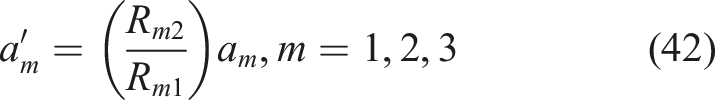
The rotor system of wind turbine has a long and heavy blade which is rotating in the vertical plane (Das et al., 2005). The vibrations of rotating wind turbine blade have been studied by several researchers, treating them as cantilever beams. The Euler–Bernoulli beam theory has been extensively used due to its simple form amongst all the beam theories (Larsen and Nielsen, 2006). However, the Rayleigh beam theory is recommended, when the influence of rotary inertia on dynamic response of the system is considered (Tang et al., 2015). The elastic body deformation of wind turbine blade is usually considered in four directions: the flapwise and edgewise deflections, and the axial and torsional deformations. The axial and torsional deformations can be ignored as the blade is relatively stiff in these directions. Meanwhile, the blade is stiffer in edgewise direction than the flapwise direction due to its cross-section (Ju and Sun, 2017).

Back in the day, studies were generally conducted on the linear model of the wind turbine blades (Krenk, 1983). Researchers became more interested in nonlinear modeling as the size of the wind turbine blade became larger. Jonkman (2003) computed the blade tip displacement, torques, and moments at the hub using the modal information of the blade vibration. Chopra and Dugundji (1979), considering the influence of nonlinearity, studied the vibration of isolated three degrees of freedom wind turbine blade under the gravity force. They showed the softening of the resonance curve and the unstable vibration because of the parametric excitation produced by the gravity field. Baumgart (2002) presented the blade as a cantilever beam which is flexible in edgewise and flapwise directions and constructed a linear dynamic model by the principle of virtual work. His model is appropriate only for the static structural analysis. Larsen and Nielsen (2006) used the Euler–Bernoulli beam model to study the wind turbine blade subjected to support motion. In their model, they included the rotation of aerodynamic load, the curvature, and the support motion, introducing geometric nonlinearity into the equation. Further, they reduced the equations of motion into a second degree of freedom system by using modal expansion, one in edgewise direction and the other in flapwise direction. Researchers (Subrahmanyam et al., 1981) found the coupled vibration frequencies and mode shapes of rotating uniform blade. They observed that the bending frequencies increase due to rotational motion.

In this work, based on Euler–Bernoulli beam theory, Hamilton’s principle is used to develop the nonlinear coupled modal equations of the rotating wind turbine blade. These equations are then expanded through orthogonal mode functions by assuming one mode in edgewise direction and two modes in flapwise direction. This work has also considered the coupling between these modes, which has been overlooked by most previous researchers. Transient vibration analysis is conducted on the coupled modes based on the National Renewable Energy Laboratory (NREL) 5-MW wind turbine using multiple-scales method under different resonance scenarios. Finally, this paper explores the effects of combined resonance on the amplitudes, robustness, and configuration (phase) makeup of a consistent primary resonance, considering different options for aerodynamic load and geometric nonlinearity.

2. The body of the mathematical modeling

2.1. Kinetic and potential energies formulations

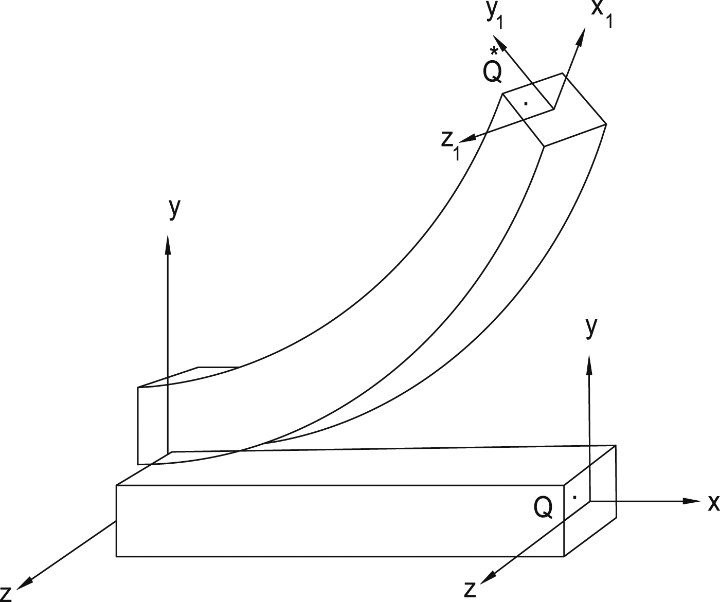
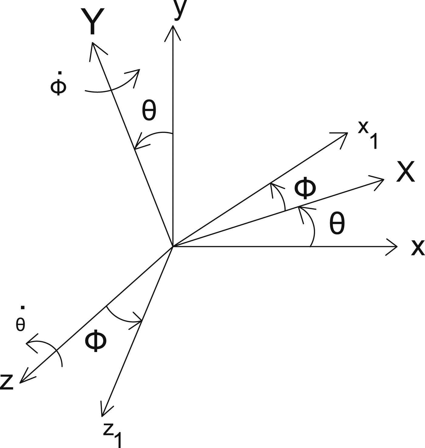
To develop the dynamic modeling of the wind turbine blade, the coordinate system $xyz$ representing the inertial frame is attached to the root of the beam, while the coordinate system $x_1{y}_1{z}_1$ is attached to the tip of the deformed beam as shown in Figure 1. The inertial coordinate system $xyz$ is aligned with the $x_1{y}_1{z}_1$ coordinate system in the undeformed configuration. Blade deformation can be described by two consecutive rigid body rotations namely $\theta$ and $\varphi$ as shown in Figure 2. Firstly, the $xyz$ coordinate system is rotated about the $z$ -axis, then about the $y_1$ -axis, the new position of the $y$ -axis as shown in Figure 2. The expressions for transformation matrix, angles $\theta$ and, elongation at point $Q$ , blade angular velocity $\left(\omega \right)$ and end curvature $\left(k\right)$ are provided in Appendix 1. An arbitrary point $Q$ in the $yz$ -plane at the tip of the beam in the undeformed configuration moves to point $Q^{*}$ in the deformed cross section as shown in Figure 1. Position vectors for points $Q$ and $Q^{*}$ are given as follows

$r_q=x\mathit{x}+Y\mathit{y}+Z\mathit{z}$

(1)

$r_{q^{*}}=x\mathit{x}+v\mathit{y}+w\mathit{z}+Y{\mathit{y}}_1+Z{\mathit{z}}_1$

(2)

Figure 1.

Blade modeled as a cantilever beam before and after deformation.

Figure 2.

Deformed to undeformed coordinate transformation by two consecutive rigid body rotations of the beam cross section.

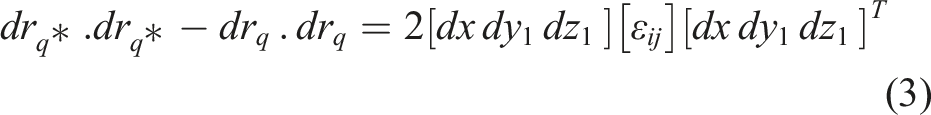
The difference of the squared distance differentials is related to the green’s strain measure as follows

$d{r}_{q^{*}}\hspace{0.17em}.d{r}_{q^{*}}-d{r}_q\hspace{0.17em}.\hspace{0.17em}d{r}_q=2\left[dx\hspace{0.17em}d{y}_1\hspace{0.17em}d{z}_1\hspace{0.17em}\right]\left[{\epsilon }_{ij}\right]{\left[dx\hspace{0.17em}d{y}_1\hspace{0.17em}d{z}_1\hspace{0.17em}\right]}^T$

(3)

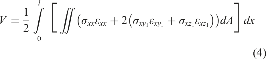
Normal stress components ${\sigma }_{YY}$ and ${\sigma }_{ZZ}$ are neglected. Hence, the total strain energy can be expressed as

$V=\frac{1}{2}\underset{0}{\overset{l}{{\displaystyle \int }}}\left[\iint \left({\sigma }_{xx}{\epsilon }_{xx}+2\left({\sigma }_{x{y}_1}{\epsilon }_{x{y}_1}+{\sigma }_{x{z}_1}{\epsilon }_{x{z}_1}\right)\right)dA\right]dx$

(4)

Linear relationship between stress and strain is assumed, therefore we can use Hooke’s law

${\sigma }_{xx}\approx E{\epsilon }_{xx},{\sigma }_{x{y}_1}\approx E{\epsilon }_{x{y}_1},{\sigma }_{x{z}_1}\approx E{\epsilon }_{x{z}_1}$

(5)

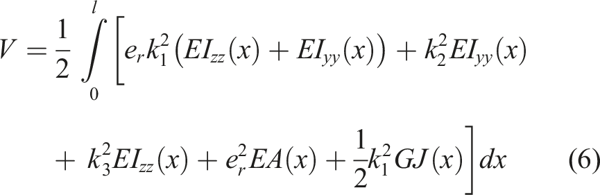
Substituting equation (3) into equation (5), and then substituting the equation (5) into equation (4), total strain energy can also be written as

$V=\frac{1}{2}\underset{0}{\overset{l}{{\displaystyle \int }}}\left[e_r{k}_1^2\left(E{I}_{zz}\left(x\right)+E{I}_{yy}\left(x\right)\right)+k_2^{2}E{I}_{yy}\left(x\right)+{\hspace{0.17em}k}_3^{2}E{I}_{zz}\left(x\right)+e_r^{2}EA\left(x\right)+\frac{1}{2}{k}_1^{2}GJ\left(x\right)\right]dx$

(6)

where $E$ , $G$ , ${{\rm I}}_{yy}\left(x\right)$ , and ${{\rm I}}_{zz}\left(x\right)$ are modulus of elasticity, shear modulus, and area moments of inertia in $y$ and $z$ directions, respectively. $e_r$ is the elongation of the beam. $k_1$ ,

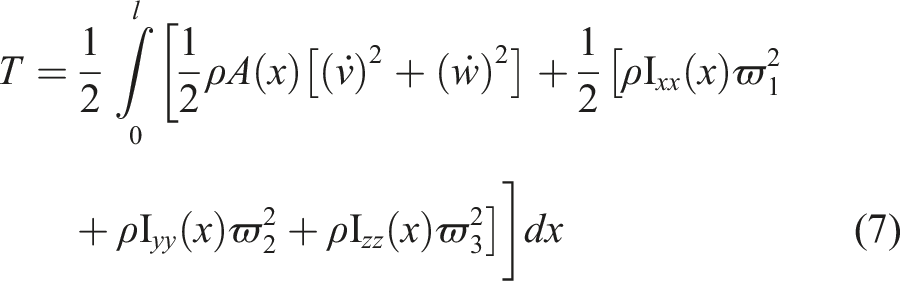
$k_2$ , $k_3$ are components of end curvature of the beam. $e_r$ , $k_1$ , $k_2$ , and $k_3$ are defined in Appendix 1. The total kinetic energy of the system is obtained as

$T=\frac{1}{2}\underset{0}{\overset{l}{{\displaystyle \int }}}\left[\frac{1}{2}\rho A\left(x\right)\left[{\left(\dot{v}\right)}^2+{\left(\dot{w}\right)}^2\right]+\frac{1}{2}\left[\rho {{\rm I}}_{xx}\left(x\right){\varpi }_1^2+\rho {{\rm I}}_{yy}\left(x\right){\varpi }_2^2+\rho {{\rm I}}_{zz}\left(x\right){\varpi }_3^2\right]\right]dx$

(7)

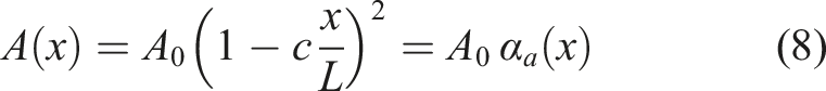
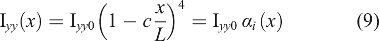
where $A$ is the cross-section area and $\rho$ is the density of the material. ${\varpi }_1$ , ${\varpi }_2$ , and ${\varpi }_3$ are angular velocities of the blade components, are defined in Appendix 1. A linear decrease from the root to the tip of the blade is assumed in the cross-section area and area moments of inertia. The assumed functions are:

$A\left(x\right)=A_0{\left(1-c\frac{x}{L}\right)}^2=A_0{\hspace{0.17em}\alpha }_a\left(x\right)$

(8)

${{\rm I}}_{yy}\left(x\right)={{\rm I}}_{yy0}{\left(1-c\frac{x}{L}\right)}^4={{\rm I}}_{yy0}{\hspace{0.17em}\alpha }_{i\hspace{0.17em}}\left(x\right)$

(9)

${{\rm I}}_{zz}\left(x\right)={{\rm I}}_{zz0}{\left(1-c\frac{x}{L}\right)}^4={{\rm I}}_{zz0}{\hspace{0.17em}\alpha }_{i\hspace{0.17em}}\left(x\right)$

(10)

where ${{\rm I}}_{yy0}$ and ${{\rm I}}_{zz0}$ are the area moments of inertia at the root of the blade and $A_0$ is the cross-section area at the root of the blade, $c$ is the shape factor that determines the amount of inertia or cross section at the tip of the blade and $L$ is the length of the blade.

2.2. Development of the governing equations using Hamilton’s principle

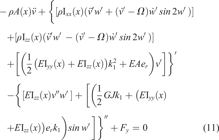
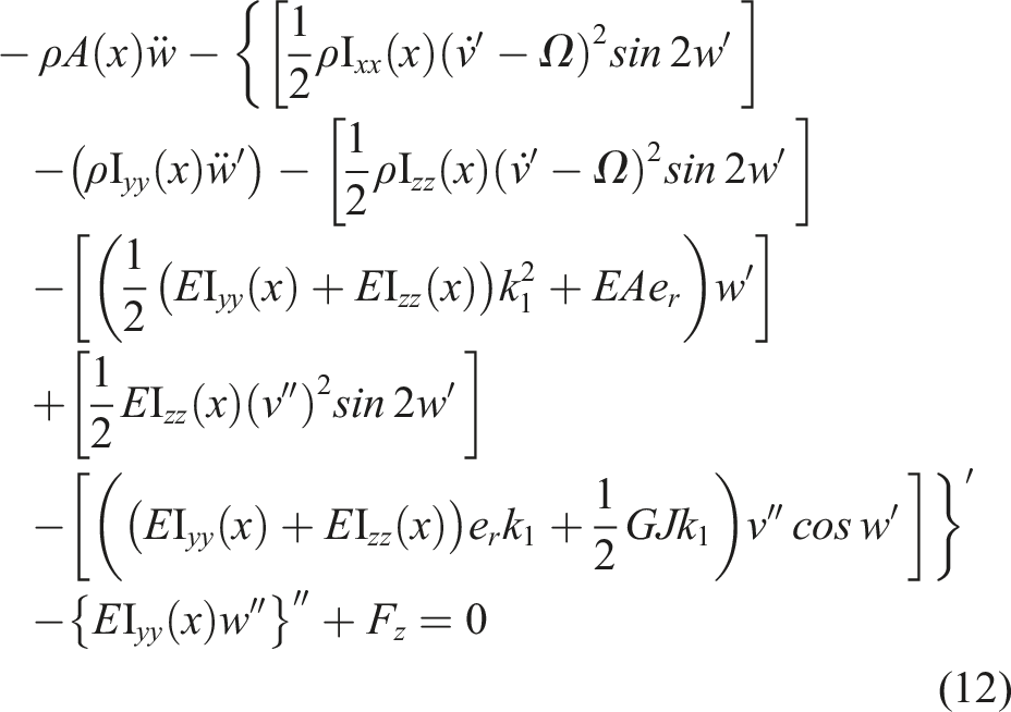
Final equations of motion for the blade vibration in the edgewise direction and flapwise direction are obtained by taking the variation of kinetic and potential energies in the $v$ and $w$ directions as

$-\rho A\left(x\right)\ddot{v}+{\left\{\left[\rho {{\rm I}}_{xx}\left(x\right)\left({\ddot{v}}^{\prime }{w}^{\prime }+\left({\dot{v}}^{\prime }-\Omega \right){\dot{w}}^{\prime }\hspace{0.17em}\mathit{sin}\hspace{0.17em}2w^{\prime }\hspace{0.17em}\right)\right]+\left[\rho {{\rm I}}_{zz}\left(x\right)\left({\ddot{v}}^{\prime }{w}^{\prime }\hspace{0.17em}-\left({\dot{v}}^{\prime }-\Omega \right){\dot{w}}^{\prime }\hspace{0.17em}\mathit{sin}\hspace{0.17em}2w^{\prime }\hspace{0.17em}\right)\right]+\left[\left(\frac{1}{2}\left(E{{\rm I}}_{yy}\left(x\right)+E{{\rm I}}_{zz}\left(x\right)\right)k_1^2+EA{e}_r\right)v^{\prime }\right]\right\}}^{\prime }-{\left\{\left[E{{\rm I}}_{zz}\left(x\right)v^{″}{w}^{\prime }\hspace{0.17em}\right]+\left[\left(\frac{1}{2}GJ{k}_1+\left(E{{\rm I}}_{yy}\left(x\right)+E{{\rm I}}_{zz}\left(x\right)\right)e_r{k}_1\right)\mathit{sin}\hspace{0.17em}{w}^{\prime }\hspace{0.17em}\right]\right\}}^{″}+F_y=0$

(11)

$-\rho A\left(x\right)\ddot{w}-{\left\{\left[\frac{1}{2}\rho {{\rm I}}_{xx}\left(x\right){\left({\dot{v}}^{\prime }-\Omega \right)}^2\mathit{sin}\hspace{0.17em}2w^{\prime }\hspace{0.17em}\right]-\left(\rho {{\rm I}}_{yy}\left(x\right){\ddot{w}}^{\prime }\right)-\left[\frac{1}{2}\rho {{\rm I}}_{zz}\left(x\right){\left({\dot{v}}^{\prime }-\Omega \right)}^2\mathit{sin}\hspace{0.17em}2w^{\prime }\hspace{0.17em}\right]-\left[\left(\frac{1}{2}\left(E{{\rm I}}_{yy}\left(x\right)+E{{\rm I}}_{zz}\left(x\right)\right)k_1^2+EA{e}_r\right)w^{\prime }\right]+\left[\frac{1}{2}E{{\rm I}}_{zz}\left(x\right){\left(v^{″}\right)}^2\mathit{sin}\hspace{0.17em}2w^{\prime }\hspace{0.17em}\right]-\left[\left(\left(E{{\rm I}}_{yy}\left(x\right)+E{{\rm I}}_{zz}\left(x\right)\right)e_r{k}_1+\frac{1}{2}GJ{k}_1\right)v^{″}\hspace{0.17em}\mathit{cos}\hspace{0.17em}{w}^{\prime }\hspace{0.17em}\right]\right\}}^{\prime }-{{\left\{E{{\rm I}}_{yy}\left(x\right)w^{″}\right\}}^{″}+F}_z=0$

(12)

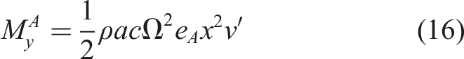
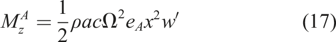
where $\Omega$ is the blade rotational speed, $F_y$ and $F_z$ are the external forces of wind and gravitation in $y$ - and $z$ - directions, respectively. $M_y$ and $M_z$ are the aerodynamic moments in edgewise and flapwise directions, respectively. The gravitational force can be expressed as

$F_y^G\left(x\right)=mgsin\left(\mathrm{\Omega }t\right),{\hspace{0.17em}F}_z^G\left(x\right)=mgsin\left({\beta }_p\right)\mathit{cos}\left(\mathrm{\Omega }t\right)$

(13)

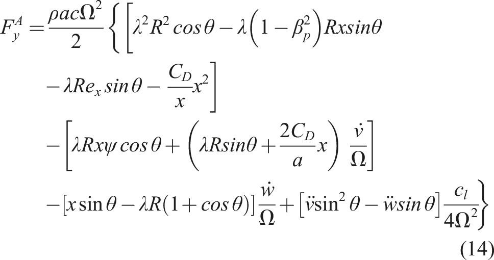
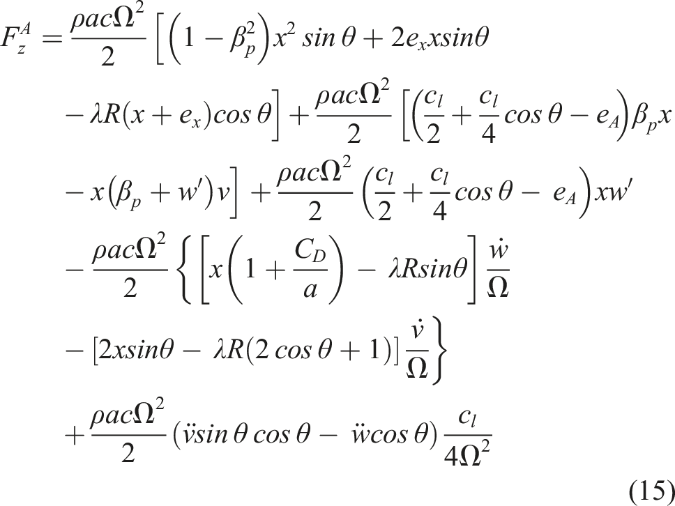
where $m$ is the distributed mass of the blade, ${\beta }_p$ is the conning angle and $g$ is the gravitational acceleration. Greenberg’s formulations, that are based on unsteady airfoil theory, are used for the aerodynamic forces and moments in the edgewise and flapwise directions (Greenberg, 1947)

$F_y^A=\frac{\rho ac{\mathrm{\Omega }}^2}{2}\left\{\left[{\lambda }^2{R}^2\hspace{0.17em}\mathit{cos}\hspace{0.17em}\theta -\lambda \left(1-{\beta }_p^2\right)Rxsin\theta -\hspace{0.17em}\lambda R{e}_x\hspace{0.17em}\mathit{sin}\hspace{0.17em}\theta -\hspace{0.17em}\frac{C_D}{x}{x}^2\right]-\left[\lambda Rx\psi \hspace{0.17em}\mathit{cos}\hspace{0.17em}\theta +\left(\lambda Rsin\theta +\frac{2C_D}{a}x\right)\frac{\dot{v}}{\mathrm{\Omega }}\right]-\left[x\hspace{0.17em}\sin \hspace{0.17em}\theta -\lambda R\left(1+\mathit{cos}\hspace{0.17em}\theta \right)\right]\frac{\dot{w}}{\mathrm{\Omega }}+\left[\ddot{v}{\sin }^2\hspace{0.17em}\theta -\ddot{w}\mathit{sin}\hspace{0.17em}\theta \right]\frac{c_l}{4{\mathrm{\Omega }}^2}\hspace{0.17em}\right\}$

(14)

$F_z^A=\frac{\rho ac{\mathrm{\Omega }}^2}{2}\left[\left(1-{\beta }_p^2\right)x^2\hspace{0.17em}\mathit{sin}\hspace{0.17em}\theta +{2e}_{x}xsin\theta -\hspace{0.17em}\lambda R\left({x+e}_x\right)\mathit{cos}\hspace{0.17em}\theta \right]+\frac{\rho ac{\mathrm{\Omega }}^2}{2}\left[\left(\frac{c_l}{2}+\frac{c_l}{4}\mathit{cos}\hspace{0.17em}\theta -\hspace{0.17em}{e}_A\right){\beta }_{p}x-x\left({\beta }_p+w^{\prime }\right)v\right]+\frac{\rho ac{\mathrm{\Omega }}^2}{2}\left(\frac{c_l}{2}+\frac{c_l}{4}\mathit{cos}\hspace{0.17em}\theta -\hspace{0.17em}{e}_A\right)x{w}^{\prime }-\hspace{0.17em}\frac{\rho ac{\mathrm{\Omega }}^2}{2}\left\{\left[x\left(1+\frac{C_D}{a}\right)-\hspace{0.17em}\lambda Rsin\theta \right]\frac{\dot{w}}{\mathrm{\Omega }}-\hspace{0.17em}\left[2xsin\theta -\hspace{0.17em}\lambda R\left(2\hspace{0.17em}\mathit{cos}\hspace{0.17em}\theta +1\right)\right]\frac{\dot{v}}{\mathrm{\Omega }}\right\}+\frac{\rho ac{\mathrm{\Omega }}^2}{2}\left(\ddot{v}\mathit{sin}\hspace{0.17em}\theta \hspace{0.17em}\mathit{cos}\hspace{0.17em}\theta -\hspace{0.17em}\ddot{w}\mathit{cos}\hspace{0.17em}\theta \right)\frac{c_l}{4{\mathrm{\Omega }}^2}$

(15)

$M_y^A=\frac{1}{2}\rho ac{\mathrm{\Omega }}^2{e}_A{x}^2{v}^{\prime }$

(16)

$M_z^A=\frac{1}{2}\rho ac{\mathrm{\Omega }}^2{e}_A{x}^2{w}^{\prime }$

(17)

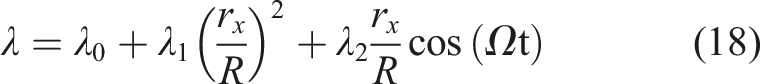
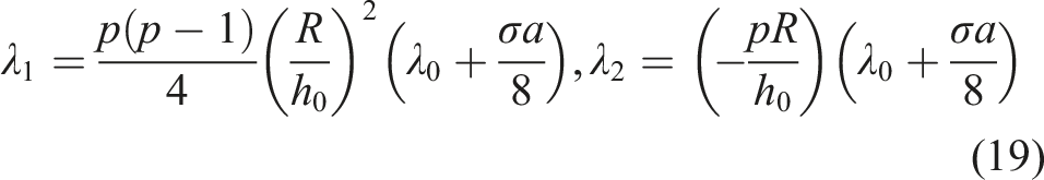
where $R$ is the rotor radius, $\rho$ is the air density, $\psi$ is the pre-twist angle, $a$ is the slope of section lift curve, and $c$ is the chord length. $C_D$ is drag coefficient and $e_A$ is the distance between the center of aerodynamic force and barycenter of the blade. The rotor inflow ratio $\lambda$ is defined as (Li et al., 2012)

$\lambda ={\lambda }_0+{\lambda }_1{\left(\frac{r_x}{R}\right)}^2+{\lambda }_2\frac{r_x}{R}\cos \hspace{0.17em}\left(\Omega \mathrm{t}\right)$

(18)

${\lambda }_1=\frac{p\left(p-1\right)}{4}{\left(\frac{R}{h_0}\right)}^2\left({\lambda }_0+\frac{\sigma a}{8}\right),{\lambda }_2=\left(-\frac{\mathit{pR}}{h_0}\right)\left({\lambda }_0+\frac{\sigma a}{8}\right)$

(19)

where ${\lambda }_0=v_0/\Omega \mathrm{R}$ is the inflow ratio at hub and $v_0$ is the inflow velocity at hub height $h_0$ . $p$ is wind shear exponent, $r_x$ is the blade radial station. $\sigma =nc/\pi R$ is the rotor solidity. $n$ is the number of wind turbine blades.

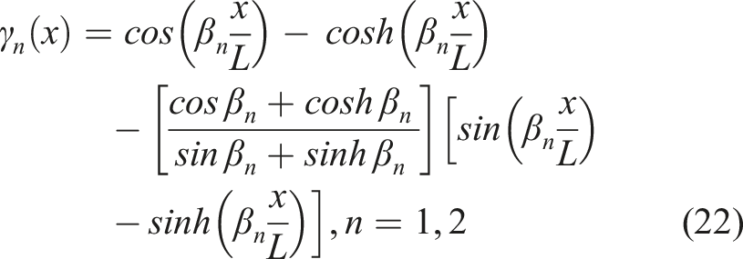
It has been observed (Jonkman et al., 2009) that the first edgewise mode and first two modes in flap-wise direction are the governing modes for wind turbine blade. Therefore, these modes are considered in this work. Mode shapes of conventional Euler–Bernoulli cantilever beam having fixed-free boundary conditions are (Hagedorn and DasGupta, 2007)

$v\left(x,t\right)={\displaystyle \sum }_1^n{\gamma }_n\left(x\right)p_n\left(t\right)={\gamma }_1\left(x\right)p_1\left(t\right)$

(20)

$w\left(x,t\right)={\displaystyle \sum }_1^n{\gamma }_n\left(x\right)q_n\left(t\right)={\gamma }_1\left(x\right)q_1\left(t\right)+{\gamma }_2\left(x\right)q_2\left(t\right)$

(21)

where $\gamma \left(x\right)$ is the orthogonal modal function, $p\left(t\right)$ and $q\left(t\right)$ are the generalized coordinates in edge and flap directions, respectively. Mode shapes of a cantilever beam having fixed-free boundary conditions are (Rao, 2007)

${\gamma }_n\left(x\right)=\mathit{cos}\left({\beta }_n\frac{x}{L}\right)-\hspace{0.17em}\mathit{cosh}\left({\beta }_n\frac{x}{L}\right)-\hspace{0.17em}\left[\frac{\mathit{cos}\hspace{0.17em}{\beta }_n+\mathit{cosh}\hspace{0.17em}{\beta }_n\hspace{0.17em}}{\mathit{sin}\hspace{0.17em}{\beta }_n+\mathit{sinh}\hspace{0.17em}{\beta }_n\hspace{0.17em}}\right]\left[\mathit{sin}\left({\beta }_n\frac{x}{L}\right)-\hspace{0.17em}\mathit{sinh}\left({\beta }_n\frac{x}{L}\right)\right],n=1,2$

(22)

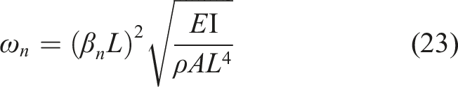
where ${\beta }_1=1.8751,{\beta }_2=4.69409$ . For Euler–Bernoulli beam with fixed-free boundary conditions, natural frequencies can be found by (Hagedorn and DasGupta, 2007)

${\omega }_n={\left({\beta }_{n}L\right)}^2\sqrt{\frac{E{\rm I}}{\rho A{L}^4}}$

(23)

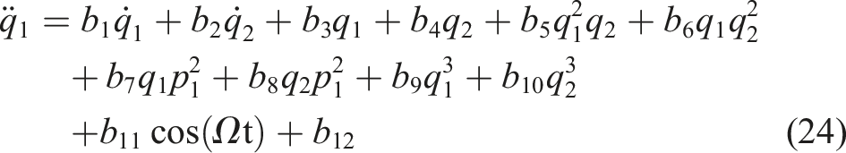
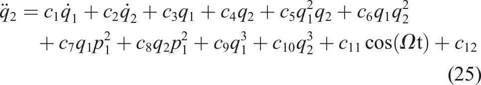
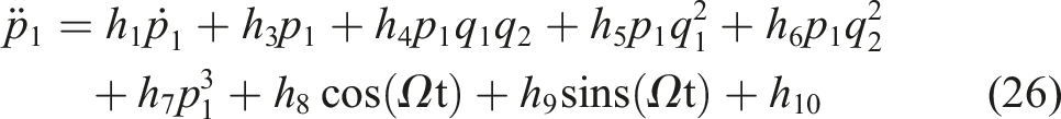
Equations (11) and (12) are reduced through Galerkin’s method as follows

${\ddot{q}}_1={b_1{\dot{q}}_1+b_2{\dot{q}}_2+b}_3{q}_1+b_4{q}_2+b_5{q}_1^2{q}_2+b_6{q}_1{q}_2^2+{\hspace{0.17em}b}_7{q}_1{p}_1^2+b_8{q}_2{p}_1^2+b_9{q}_1^3+b_{10}{q}_2^3+b_{11}\hspace{0.17em}\cos \left(\Omega \mathrm{t}\right)+b_{12}$

(24)

${\ddot{q}}_2={c_1{\dot{q}}_1+c_2{\dot{q}}_2+c}_3{q}_1+c_4{q}_2+c_5{q}_1^2{q}_2+c_6{q}_1{q}_2^2+c_7{q}_1{p}_1^2+c_8{q}_2{p}_1^2+c_9{q}_1^3+c_{10}{q}_2^3+c_{11}\hspace{0.17em}\cos \left(\Omega \mathrm{t}\right)+c_{12}$

(25)

${\ddot{p}}_1={h_1{\dot{p}}_1+h}_3{p}_1+h_4{p}_1{q}_1{q}_2+h_5{p}_1{q}_1^2+h_6{p}_1{q}_2^2+h_7{p}_1^3+h_8\hspace{0.17em}\cos \left(\Omega \mathrm{t}\right)+h_9\text{sins}\left(\Omega \mathrm{t}\right)+h_{10}$

(26)

The coefficients $b_i\left(i=1,\dots ,12\right)$ , $c_j\left(j=1,\dots ,12\right)$ , and $h_k\left(k=1,\dots ,10\right)$ are defined in Appendix 2. The linear natural frequencies of first flap mode ( ${\omega }_1$ ), second flap mode ( ${\omega }_2$ ), and first edge mode ( ${\omega }_3$ ) are also defined in Appendix 3.

3. Multiple-scales method to obtain the analytical solution

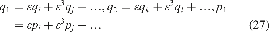
Multiple-scales perturbation method is used to solve equations (24)–(26). Aerodynamic forces are scaled to be the order of $\epsilon$ . Displacements are assumed as

$q_1=\epsilon q_i+{\epsilon }^3{q}_j+\dots ,q_2=\epsilon q_k+{\epsilon }^3{q}_l+\dots ,p_1=\epsilon p_i+{\epsilon }^3{p}_j+\dots$

(27)

$b_{11}=\epsilon b_{11},c_{11}=\epsilon c_{11},h_8=\epsilon h_8,h_9=\epsilon h_9$

(28)

where $\epsilon$ is a small scaling parameter, two different time scales $t_0=t$ and $t_2={\epsilon }^{2}t$ are adopted. Responses $q_i$ , $q_k$ , and $p_i$ of equation (27) are obtained using multiple-scales method. Equations (27) and (28) are substituted into equations (24)–(26) and equating the coefficients of $\epsilon$ and ${\epsilon }^3$ , we get

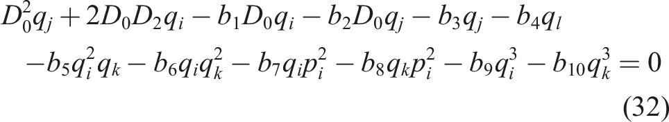
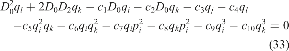
Order $\epsilon$

${D_0^{2}q}_i-b_3{q}_i-b_4{q}_k=b_{11}\hspace{0.17em}\cos \hspace{0.17em}\left(\mathrm{\Omega }t\right)$

(29)

${D_0^{2}q}_k-c_3{q}_i-c_4{q}_k=c_{11}\hspace{0.17em}\cos \hspace{0.17em}\left(\mathrm{\Omega }t\right)$

(30)

${D_0^{2}p}_i-h_3{p}_i=h_8\hspace{0.17em}\cos \left(\Omega \mathrm{t}\right)+h_9\hspace{0.17em}\sin \hspace{0.17em}\left(\mathrm{\Omega }\mathrm{t}\right)$

(31)

Order ${\epsilon }^3$

${D_0^{2}q}_j+2D_0{D}_2{q}_i-b_1{D}_0{q}_i-b_2{D}_0{q}_j-b_3{q}_j-b_4{q}_l-{{b_{5}q}_i^{2}q}_k-b_6{q}_i{q}_k^2-b_7{q}_i{p}_i^2-b_8{q}_k{p}_i^2-b_9{q}_i^3-b_{10}{q}_k^3=0$

(32)

${D_0^{2}q}_l+2D_0{D}_2{q}_k-c_1{D}_0{q}_i-c_2{D}_0{q}_k-c_3{q}_j-c_4{q}_l-{{c_{5}q}_i^{2}q}_k-c_6{q}_i{q}_k^2-c_7{q}_i{p}_i^2-c_8{q}_k{p}_i^2-c_9{q}_i^3-c_{10}{q}_k^3=0$

(33)

${D_0^{2}p}_j+2D_0{D}_2{p}_i-h_1{D}_0{p}_i-h_3{p}_j-h_4{p}_i{q}_i{q}_k-h_5{p}_i{q}_i^2-h_6{p}_i{q}_k^2-h_7{p}_i^3=0$

(34)

Solving equations (29)–(31), leads to the responses as

$q_i={\alpha }_1\left(t_2\right)e^{i{\omega }_1{t}_0}+{\alpha }_2\left(t_2\right)e^{i{\omega }_2{t}_0}{+{\mathrm{\Gamma }}_{1}e}^{i\mathrm{\Omega }{t}_0}+c.c.$

(35)

$q_k={{\mathrm{\Lambda }}_1\alpha }_1\left(t_2\right)e^{i{\omega }_1{t}_0}+{\mathrm{\Lambda }}_2{\alpha }_2\left(t_2\right)e^{i{\omega }_2{t}_0}{+{\mathrm{\Gamma }}_{2}e}^{i\mathrm{\Omega }{t}_0}+c.c.$

(36)

$p_i={\alpha }_3\left(t_2\right)e^{i{\omega }_3{t}_0}+{\left({\mathrm{d}}_1-i{d}_2\right)e}^{i\mathrm{\Omega }{t}_0}+c.c.$

(37)

Coefficients ${\mathrm{\Lambda }}_1$ , ${\mathrm{\Lambda }}_2$ , ${\mathrm{\Gamma }}_1$ , ${\mathrm{\Gamma }}_2$ , ${\mathrm{d}}_1$ , and ${\mathrm{d}}_2$ of equations (35)–(37) are defined in Appendix 3.

3.1. Non-resonant case

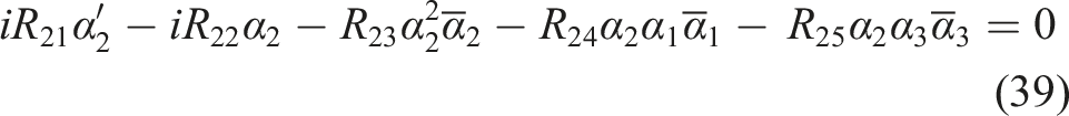
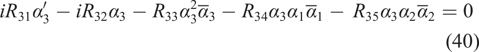
In this case, there is no specific relationship between the natural frequencies of the system. Substituting equations (35)–(37) into equations (32)–(34) and equating the coefficients of $e^{i{\omega }_1{t}_0}$ , $e^{i{\omega }_2{t}_0}$ and $e^{i{\omega }_3{t}_0}$ , yields to three equations

$i{R}_{11}{\alpha }_1^{\prime }-i{R}_{12}{\alpha }_1-R_{13}{\alpha }_1^2{\overline{\alpha }}_1-R_{14}{\alpha }_1{\alpha }_2{\overline{\alpha }}_2-{\hspace{0.17em}R}_{15}{\alpha }_1{\alpha }_3{\overline{\alpha }}_3=0$

(38)

$i{R}_{21}{\alpha }_2^{\prime }-i{R}_{22}{\alpha }_2-R_{23}{\alpha }_2^2{\overline{\alpha }}_2-R_{24}{\alpha }_2{\alpha }_1{\overline{\alpha }}_1-{\hspace{0.17em}R}_{25}{\alpha }_2{\alpha }_3{\overline{\alpha }}_3=0$

(39)

$i{R}_{31}{\alpha }_3^{\prime }-i{R}_{32}{\alpha }_3-R_{33}{\alpha }_3^2{\overline{\alpha }}_3-R_{34}{\alpha }_3{\alpha }_1{\overline{\alpha }}_1-{\hspace{0.17em}R}_{35}{\alpha }_3{\alpha }_2{\overline{\alpha }}_2=0$

(40)

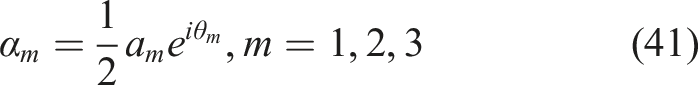
To solve equations (38)–(40), we assume amplitudes as

${\alpha }_m=\frac{1}{2}{a}_m{e}^{i{\theta }_m},m=1,2,3$

(41)

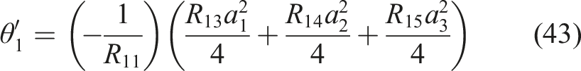
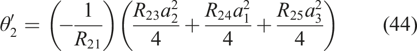
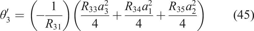
Substituting equation (41) into equations (38)–(40), and equating the real and imaginary parts, one obtains

$a_m^{\prime }=\left(\frac{R_{m2}}{R_{m1}}\right)a_m,m=1,2,3$

(42)

${\theta }_1^{\prime }=\left(-\frac{1}{R_{11}}\right)\left(\frac{R_{13}{a}_1^2}{4}+\frac{R_{14}{a}_2^2}{4}+\frac{R_{15}{a}_3^2}{4}\right)$

(43)

${\theta }_2^{\prime }=\left(-\frac{1}{R_{21}}\right)\left(\frac{R_{23}{a}_2^2}{4}+\frac{R_{24}{a}_1^2}{4}+\frac{R_{25}{a}_3^2}{4}\right)$

(44)

${\theta }_3^{\prime }=\left(-\frac{1}{R_{31}}\right)\left(\frac{R_{33}{a}_3^2}{4}+\frac{R_{34}{a}_1^2}{4}+\frac{R_{35}{a}_2^2}{4}\right)$

(45)

where $a_m$ and ${\theta }_m$ are real functions of time $t_2$ . Coefficients $R_{nm}$ can be found in Appendix 3. Foregoing equations (42)–(45) can be solved numerically, the first order approximation of the response is obtained as

$q_i=\epsilon a_m\hspace{0.17em}\cos \left({\omega }_{m}t+{\theta }_m\right)+O\left({\epsilon }^3\right),m=1,2$

(46)

$q_k=\epsilon {{\mathrm{\Gamma }}_{m}a}_m\hspace{0.17em}\cos \left({\omega }_{m}t+{\theta }_m\right)+O\left({\epsilon }^3\right),m=1,2$

(47)

$p_i=\epsilon a_3\hspace{0.17em}\cos \left({\omega }_{3}t+{\theta }_3\right)+O\left({\epsilon }^3\right)$

(48)

3.2. Internal resonance between all modes, ${\omega }_1+2{\omega }_3={\omega }_2$

In this case, it is assumed that the sum of the first flapwise frequency and twice the first edgewise frequency is approximately equals to the second flapwise frequency. We detune the frequency as

${\omega }_1+{2\omega }_3={\omega }_2+{{\epsilon }^2\sigma }_1$

(49)

where ${{\epsilon }^2\sigma }_1$ is a small detuning parameter. Using the same methodology of solving equations (42)–(45), the amplitudes $a_m$ and phases ${\theta }_m$ can be obtained by solving the following equations

$a_1^{\prime }=\left(\frac{R_{12}}{R_{11}}\right)a_1+\left(\frac{R_{16}}{{4R}_{11}}\right)a_2{a}_3^2\hspace{0.17em}\mathit{sin}\hspace{0.17em}{\beta }_2$

(50)

$a_2^{\prime }=\left(\frac{R_{22}}{R_{21}}\right)a_2-\left(\frac{R_{26}}{{4R}_{21}}\right)a_1{a}_3^2\hspace{0.17em}\mathit{sin}\hspace{0.17em}{\beta }_2$

(51)

$a_3^{\prime }=\left(\frac{R_{32}}{R_{31}}\right)a_3+\left(\frac{R_{36}}{{4R}_{31}}\right)a_1{a}_2{a}_3\hspace{0.17em}\mathit{sin}\hspace{0.17em}{\beta }_2$

(52)

${\beta }_1^{\prime }=-\left(\frac{R_1}{R_{11}}\right)-\left(\frac{R_{13}}{{4R}_{11}}\right)a_1^2-\left(\frac{R_{14}}{{4R}_{11}}\right)a_2^2-\left(\frac{R_{15}}{{4R}_{11}}\right)a_3^2-\hspace{0.17em}\left(\frac{R_{16}}{{4R}_{11}}\right)\left(\frac{{a_{2}a}_3^2}{a_1}\right)\mathit{cos}\hspace{0.17em}{\beta }_2$

(53)

${\beta }_2^{\prime }=-\left(\frac{R_2}{R_{21}}\right)-\left(\frac{R_{23}}{{4R}_{21}}\right)a_2^2-\left(\frac{R_{24}}{{4R}_{21}}\right)a_1^2-\left(\frac{R_{25}}{{4R}_{21}}\right)a_3^2-\hspace{0.17em}\left(\frac{R_{26}}{{4R}_{21}}\right)\left(\frac{{a_{1}a}_3^2}{a_2}\right)\mathit{cos}\hspace{0.17em}{\beta }_2$

(54)

${\beta }_3^{\prime }=-\left(\frac{R_3}{R_{31}}\right)-\left(\frac{R_{33}}{{4R}_{31}}\right)a_3^2-\left(\frac{R_{34}}{{4R}_{31}}\right)a_1^2-\left(\frac{R_{35}}{{4R}_{31}}\right)a_2^2-\hspace{0.17em}\left(\frac{R_{36}}{{4R}_{31}}\right)a_1{a}_2\hspace{0.17em}\mathit{cos}\hspace{0.17em}{\beta }_2$

(55)

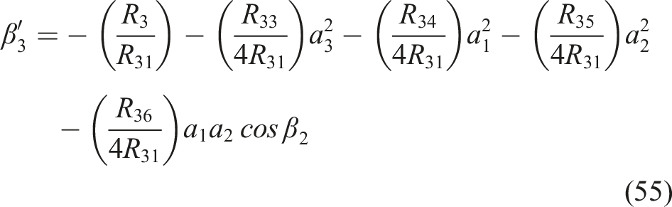
where ${{\beta }_1=\theta }_1,{\beta }_2={\theta }_2-{\theta }_1-{2\theta }_3-{\sigma }_1{t}_2\hspace{0.17em}and\hspace{0.17em}{\beta }_3={\theta }_3$ . Coefficients of equations (50)–(55) are given in Appendix 3.

3.3. Primary resonance between first edgewise frequency and blade rotational frequency, $\Omega ={\omega }_3$

In the primary resonance case, the rotational frequency of blade is near the natural frequency of one of the blade modes. In this study, we consider the first edgewise frequency. We detune the blade rotational frequency as given

$\mathrm{\Omega }={\omega }_3+{{\epsilon }^2\sigma }_2$

(56)

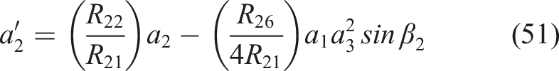
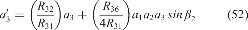
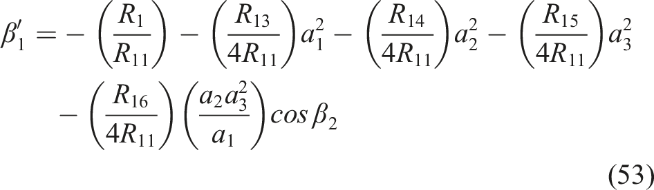
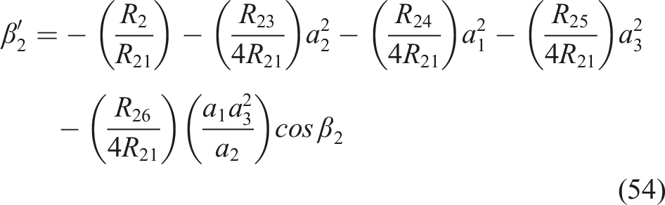
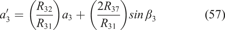
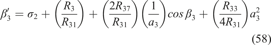
where ${{\epsilon }^2\sigma }_2$ is another detuning parameter. Employing the similar approach as the previous section, the following amplitude and phase equations can be established

$a_3^{\prime }=\left(\frac{R_{32}}{R_{31}}\right)a_3+\left(\frac{2R_{37}}{R_{31}}\right)\mathit{sin}\hspace{0.17em}{\beta }_3$

(57)

${\beta }_3^{\prime }={\sigma }_2+\left(\frac{R_3}{R_{31}}\right)+\left(\frac{{2R}_{37}}{R_{31}}\right)\left(\frac{1}{a_3}\right)\mathit{cos}\hspace{0.17em}{\beta }_3+\left(\frac{R_{33}}{{4R}_{31}}\right)a_3^2$

(58)

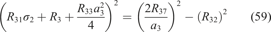
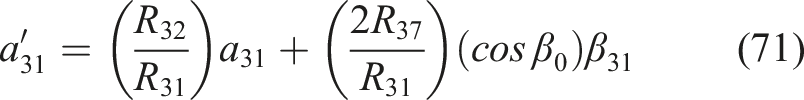
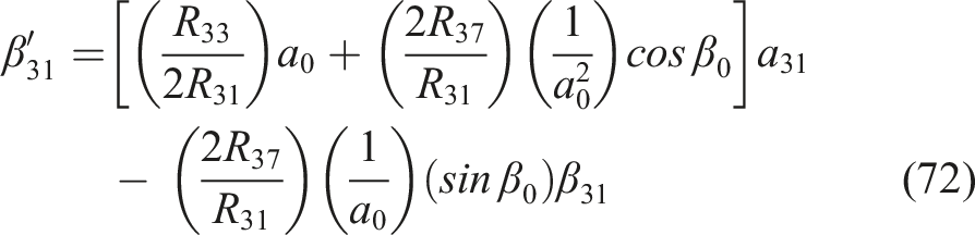
where ${\beta }_3={\sigma }_2{t}_1-{\theta }_3$ . The coefficients of equations (57) and (58) can be found in Appendix 3. The steady-state response can be obtained by letting $a_3^{\prime }={\beta }_3^{\prime }=0$ as

${\left({R_{31}\sigma }_2+R_3+\frac{R_{33}{a}_3^2}{4}\right)}^2={\left(\frac{2R_{37}}{a_3}\right)}^2-{\left(R_{32}\right)}^2$

(59)

First approximation of the steady-state solution is given by

$p_i=a_3\hspace{0.17em}\cos \left(\mathrm{\Omega }t-{\beta }_3\right)+O\left({\epsilon }^3\right)$

(60)

3.4. Combination resonance—combined internal and primary resonances, ${\omega }_1+2{\omega }_3={\omega }_2$ and $\Omega ={\omega }_3$

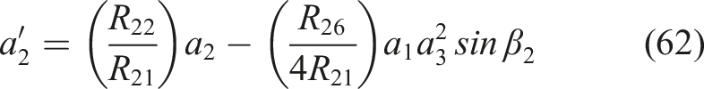
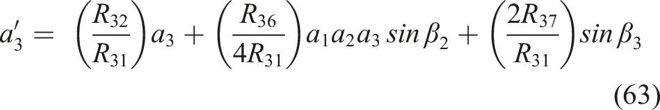
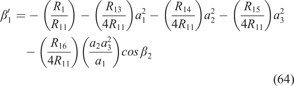
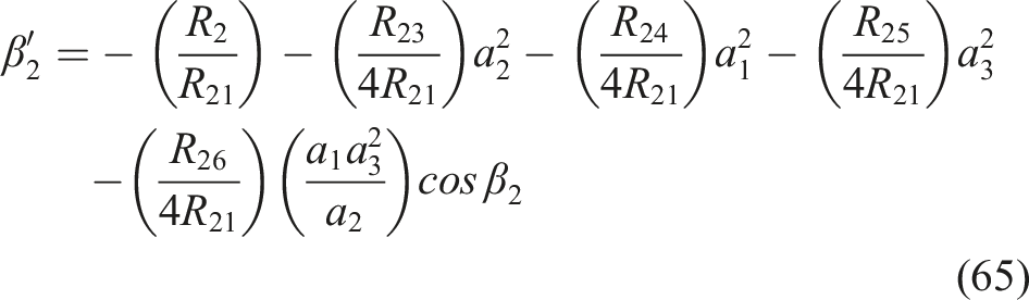
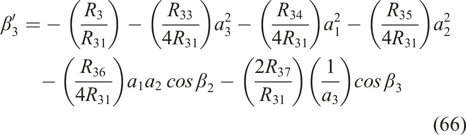
In this case, both internal and primary resonances are considered. Using same approach as in the previous section, amplitudes and phases equations can be established as

$a_1^{\prime }=\left(\frac{R_{12}}{R_{11}}\right)a_1+\left(\frac{R_{16}}{{4R}_{11}}\right)a_2{a}_3^2\hspace{0.17em}\mathit{sin}\hspace{0.17em}{\beta }_2$

(61)

$a_2^{\prime }=\left(\frac{R_{22}}{R_{21}}\right)a_2-\left(\frac{R_{26}}{{4R}_{21}}\right)a_1{a}_3^2\hspace{0.17em}\mathit{sin}\hspace{0.17em}{\beta }_2$

(62)

$a_3^{\prime }=\left(\frac{R_{32}}{R_{31}}\right)a_3+\left(\frac{R_{36}}{{4R}_{31}}\right)a_1{a}_2{a}_3\hspace{0.17em}\mathit{sin}\hspace{0.17em}{\beta }_2+\left(\frac{2R_{37}}{R_{31}}\right)\mathit{sin}\hspace{0.17em}{\beta }_3$

(63)

${\beta }_1^{\prime }=-\left(\frac{R_1}{R_{11}}\right)-\left(\frac{R_{13}}{{4R}_{11}}\right)a_1^2-\left(\frac{R_{14}}{{4R}_{11}}\right)a_2^2-\left(\frac{R_{15}}{{4R}_{11}}\right)a_3^2-\hspace{0.17em}\left(\frac{R_{16}}{{4R}_{11}}\right)\left(\frac{{a_{2}a}_3^2}{a_1}\right)\mathit{cos}\hspace{0.17em}{\beta }_2$

(64)

${\beta }_2^{\prime }=-\left(\frac{R_2}{R_{21}}\right)-\left(\frac{R_{23}}{{4R}_{21}}\right)a_2^2-\left(\frac{R_{24}}{{4R}_{21}}\right)a_1^2-\left(\frac{R_{25}}{{4R}_{21}}\right)a_3^2-\left(\frac{R_{26}}{{4R}_{21}}\right)\left(\frac{{a_{1}a}_3^2}{a_2}\right)\mathit{cos}\hspace{0.17em}{\beta }_2$

(65)

${\beta }_3^{\prime }=-\left(\frac{R_3}{R_{31}}\right)-\left(\frac{R_{33}}{{4R}_{31}}\right)a_3^2-\left(\frac{R_{34}}{{4R}_{31}}\right)a_1^2-\left(\frac{R_{35}}{{4R}_{31}}\right)a_2^2-\hspace{0.17em}\left(\frac{R_{36}}{{4R}_{31}}\right)a_1{a}_2\hspace{0.17em}\mathit{cos}\hspace{0.17em}{\beta }_2-\left(\frac{{2R}_{37}}{R_{31}}\right)\left(\frac{1}{a_3}\right)\mathit{cos}\hspace{0.17em}{\beta }_3$

(66)

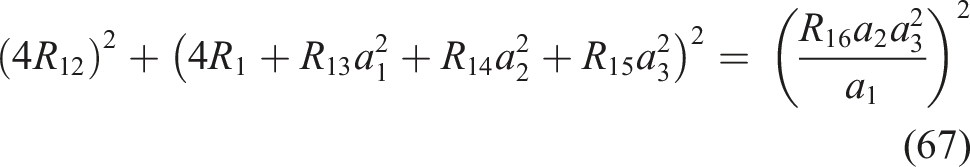
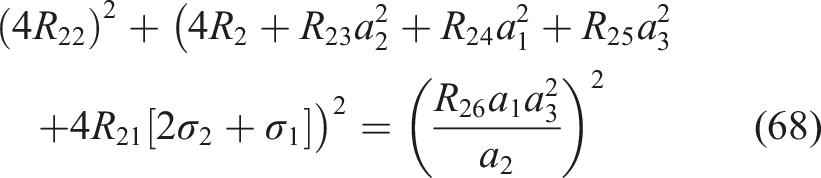
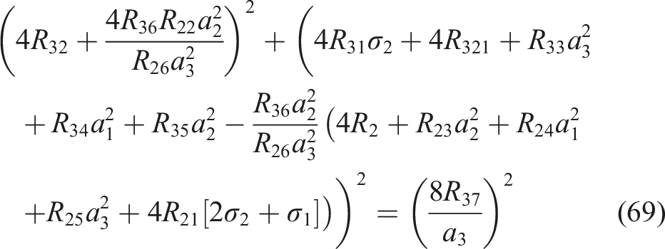
where ${{\beta }_1=\theta }_1,{\beta }_2={\theta }_2-{\theta }_1-{2\theta }_3-{\sigma }_1{t}_2,{\beta }_3={\sigma }_2{t}_2-{\theta }_3$ . The coefficients of equations (61)–(66) are defined in Appendix 3. The steady-state responses can be obtained by letting $a_{1-3}^{\prime }={\theta }_{1-3}^{\prime }=0$ as

${\left({4R}_{12}\right)}^2+{\left(4R_1+R_{13}{a}_1^2+R_{14}{a}_2^2+R_{15}{a}_3^2\right)}^2={\hspace{0.17em}\left(\frac{R_{16}{a_{2}a}_3^2}{a_1}\right)}^2$

(67)

${\left({4R}_{22}\right)}^2+{\left(4R_2+R_{23}{a}_2^2+R_{24}{a}_1^2+R_{25}{a}_3^2+4R_{21}\left[2{\sigma }_2+{\sigma }_1\right]\right)}^2={\left(\frac{R_{26}{a_{1}a}_3^2}{a_2}\right)}^2$

(68)

${\left({4R}_{32}+\frac{4R_{36}{R}_{22}{a}_2^2}{R_{26}{a}_3^2}\right)}^2+{\left({4R_{31}\sigma }_2+4R_{321}+R_{33}{a}_3^2+{\hspace{0.17em}R}_{34}{a}_1^2+R_{35}{a}_2^2-\frac{R_{36}{a}_2^2}{R_{26}{a}_3^2}\left(4R_2+R_{23}{a}_2^2+R_{24}{a}_1^2+R_{25}{a}_3^2+4R_{21}\left[2{\sigma }_2+{\sigma }_1\right]\right)\right)}^2={\left(\frac{{8R}_{37}}{a_3}\right)}^2$

(69)

Newton’s method is used to solve equations (59) and (67)–(69).

4. Results and discussions

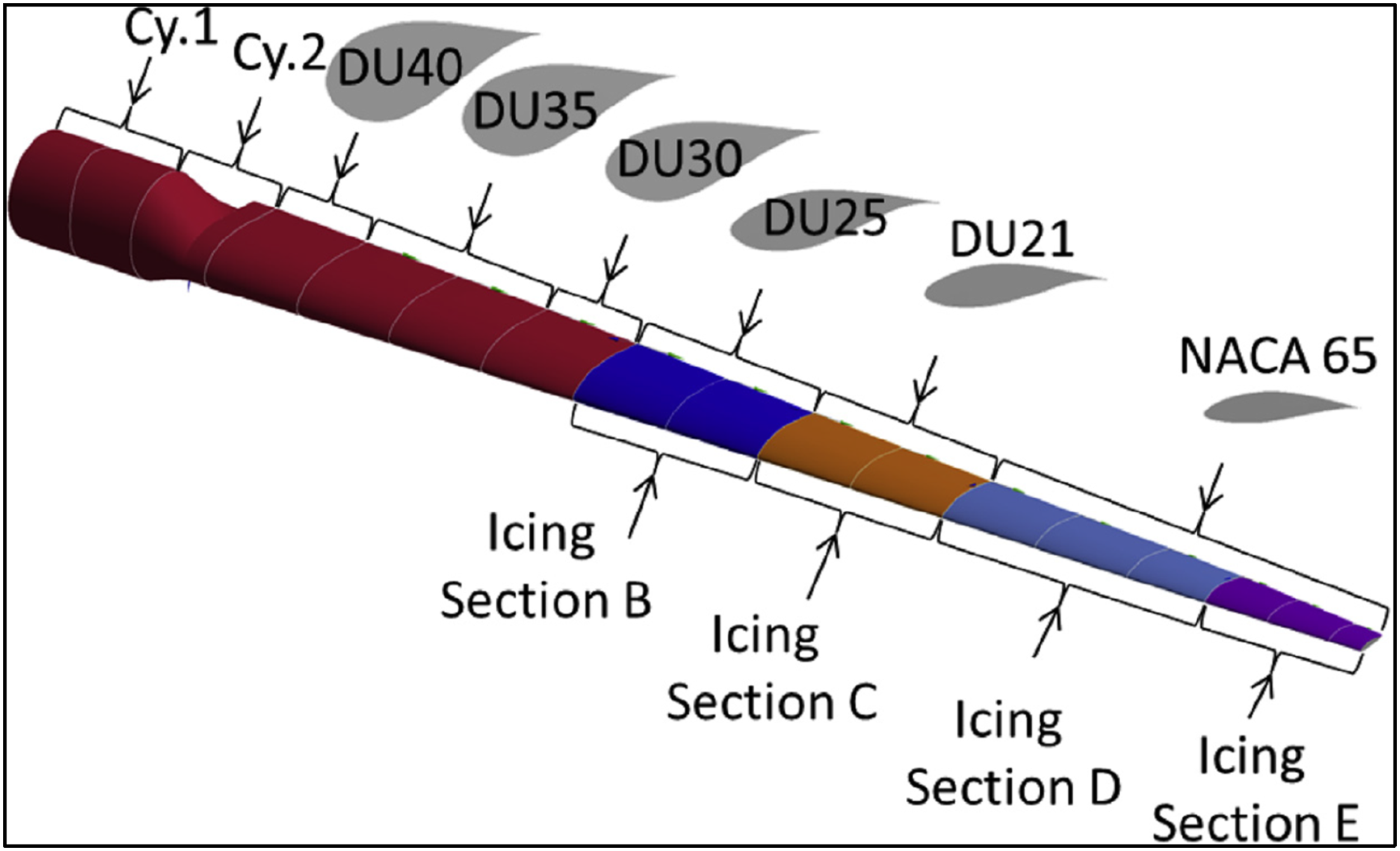
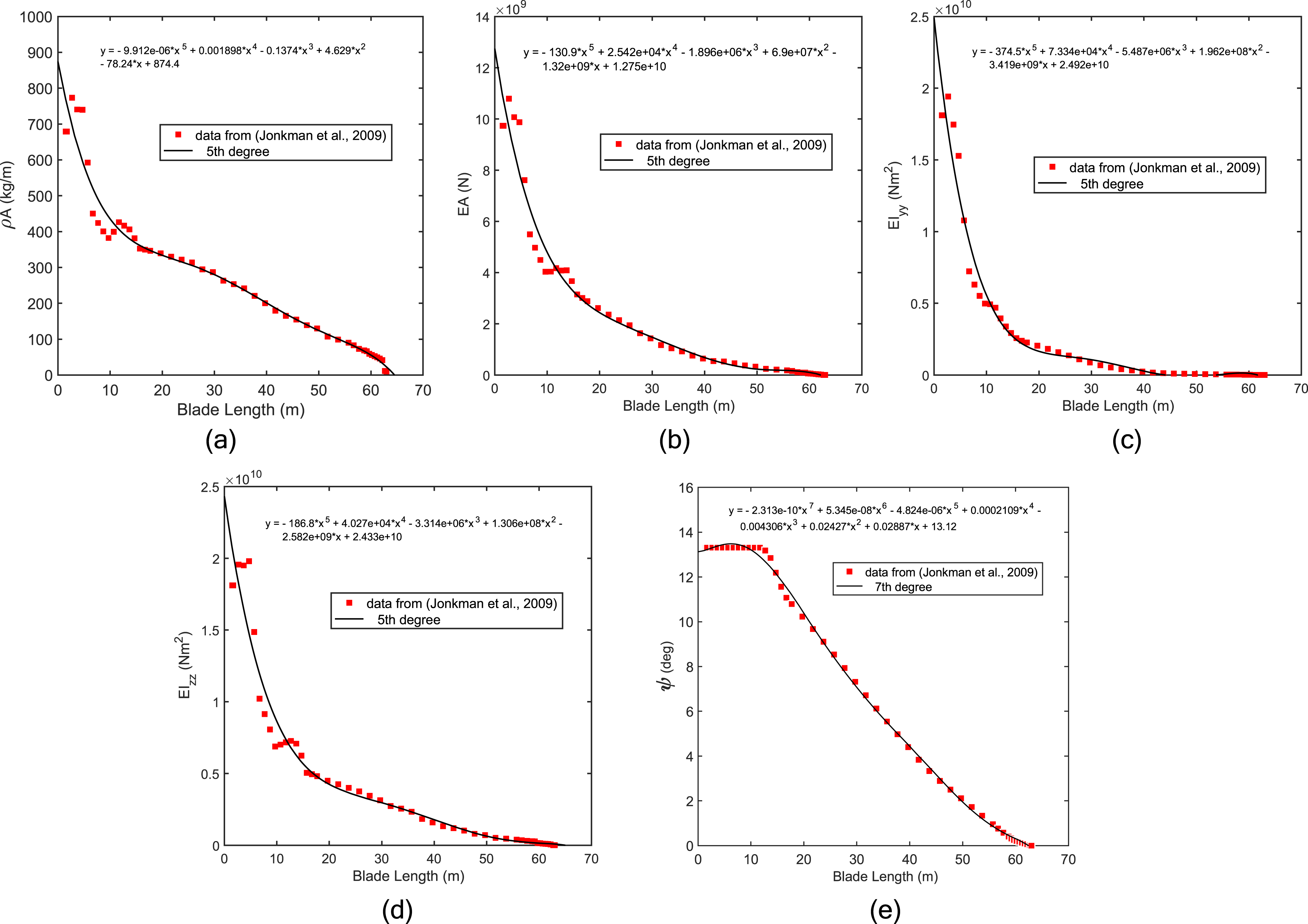
Numerical values of the structural specifications of NREL-5 MW horizontal axis wind turbine are used. Blade is discretized into 17 sections and 8 different aero foils were used to form these segments as shown in Figure 3 (Zanon et al., 2018). Blade length is assumed as $L=51.3\hspace{0.17em}m$ and blade root length as $r=11.7\hspace{0.17em}m$ . Root values of mass density, edgewise stiffness, and flapwise stiffness are defined as: $\rho A_0=426.32\hspace{0.17em}kg/m,E{I}_{yy0}=7167.7\times {10}^6\hspace{0.17em}N{m}^2,E{I}_{zz0}=4691.7\times {10}^6\hspace{0.17em}N{m}^2$ . Figure 4 shows the plot of these values. Conning angle $\left({\beta }_p\right)$ , blade speed $\left(\Omega \right)$ , and inflow wind speed $\left(v_0\right)$ are $-{2.5}^0$ , $12.1\hspace{0.17em}rpm$ , and $11.4\hspace{0.17em}m/s$ , respectively.

Figure 3.

NREL-5 MW wind turbine blade with sections and aero foils (Zanon et al., 2018).

Figure 4.

Plots of NREL-5 MW wind turbine blade data (Jonkman et al., 2009) for (a): mass per unit length, (b): axial stiffness, (c): flapwise flexural rigidity, (d): edgewise flexural rigidity.

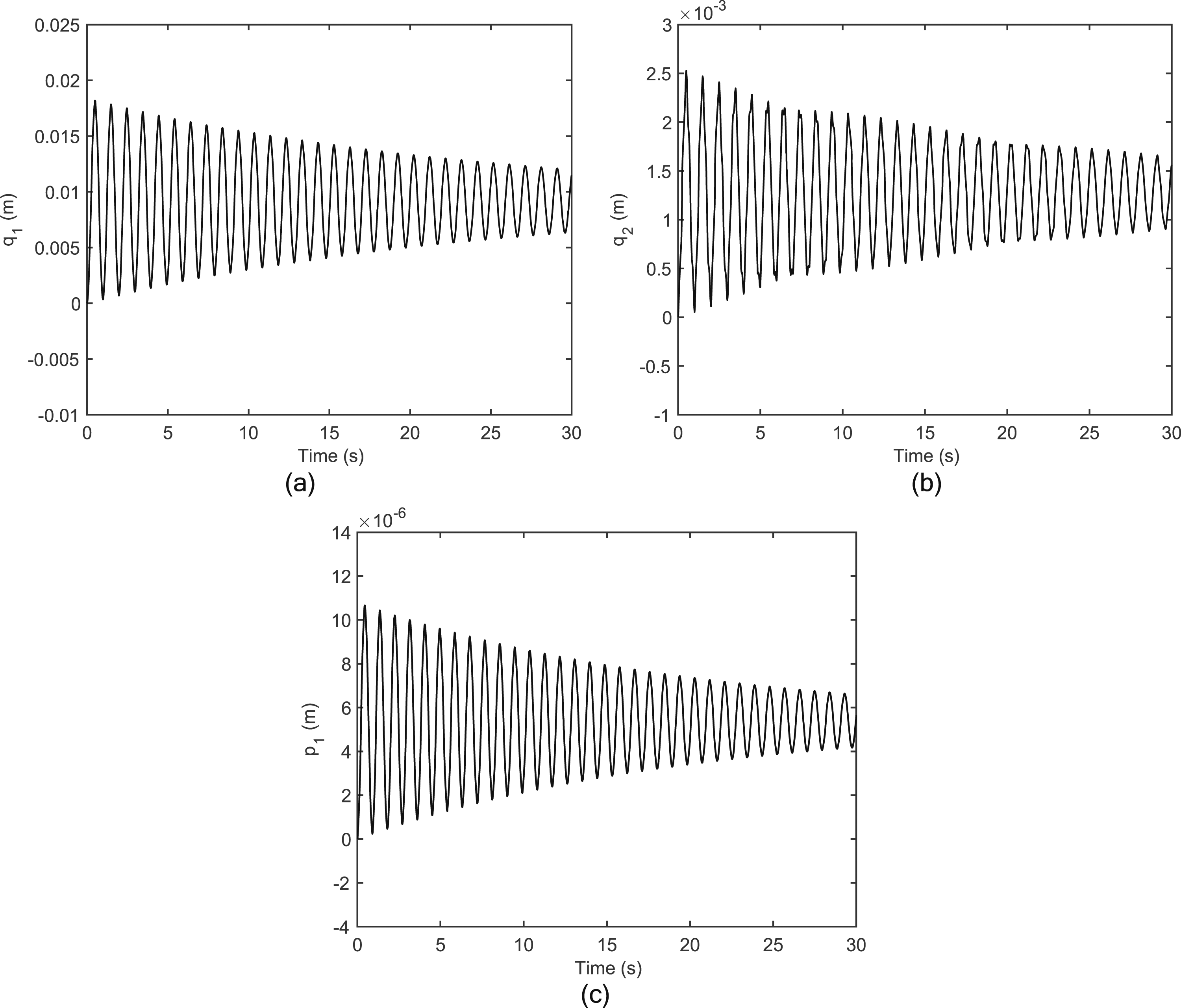
Figures 5–7 represent total deflections under combined gravity and inflow wind. Blade modal natural frequencies are tabulated in Table 1. The discrepancy is small between the calculated frequencies and the ones found in reference work (Resor, 2013).

Figure 5.

Blade tip vibration under combine gravity and inflow wind loads for (a): first flapwise mode, (b): second flapwise mode, (c): first edgewise mode.

Figure 6.

Blade tip vibration due to gravity load for (a): first flapwise mode, (b): second flapwise mode, (c): first edgewise mode.

Figure 7.

Blade tip vibration due to aerodynamic load for (a): first flapwise mode, (b): second flapwise mode, (c): first edgewise mode.

Table 1.

The Blade modal natural frequencies in Hertz.

Mode	Description	Frequency calculated in this work (Hz)	Frequency given in (Resor, 2013) (Hz)
1	First edgewise bending	1.005	1.06
2	First flapwise bending	0.8515	0.87
3	Second flapwise bending	2.6612	2.68

4.1. Transient responses

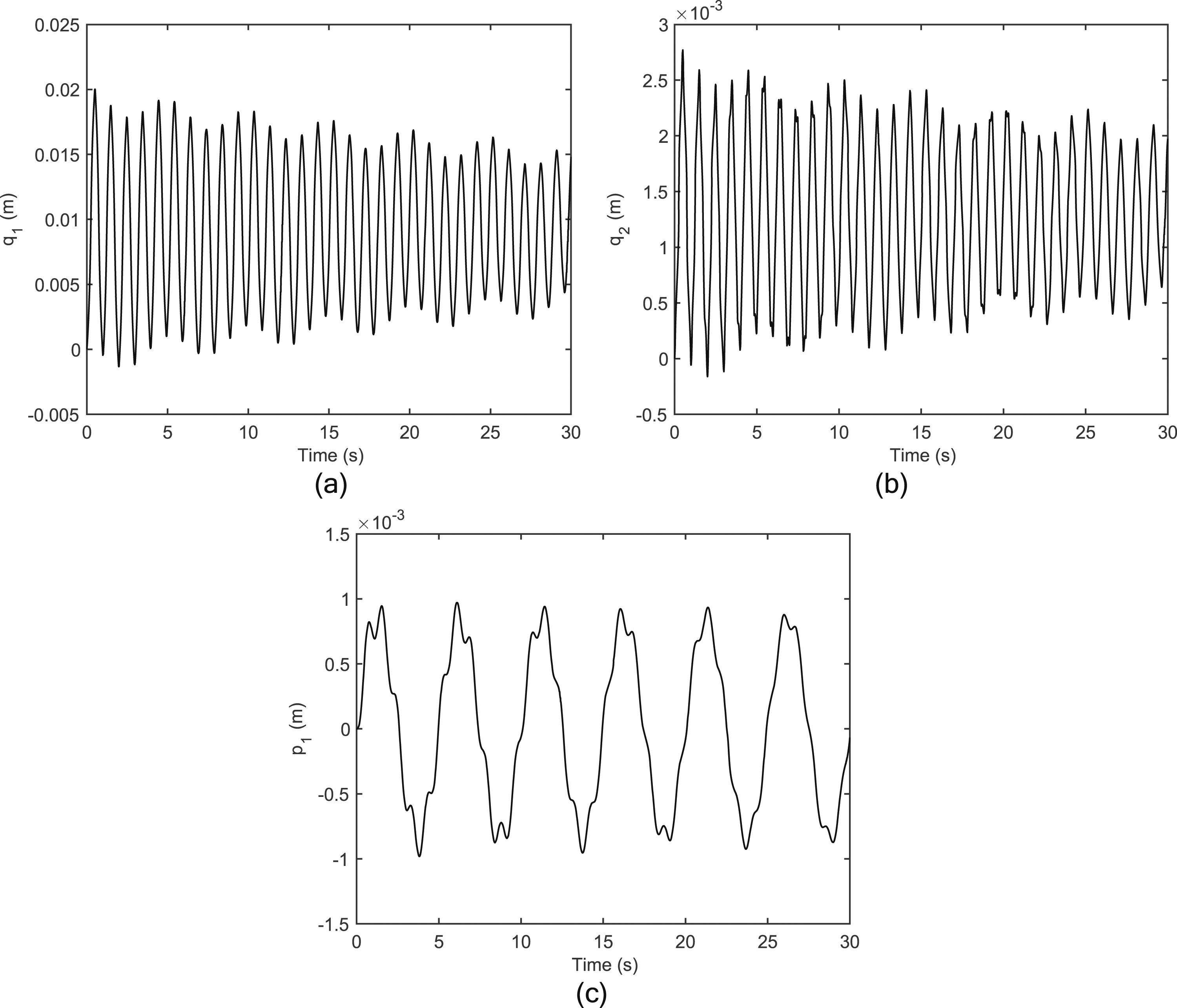
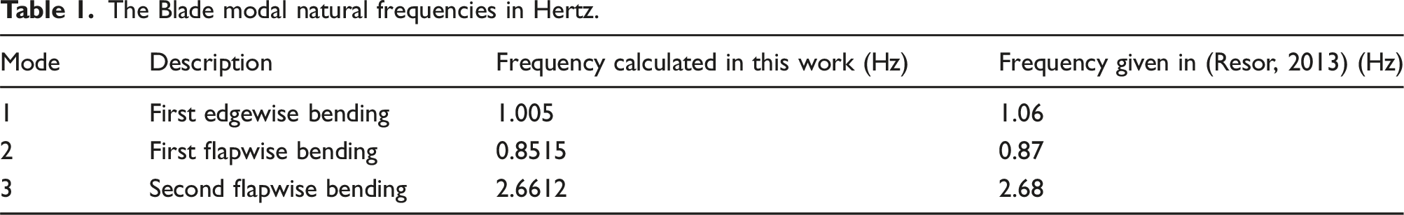
Transient oscillations occur because of the fluctuating aerodynamic force. In the non-resonant case, 42–45 are solved using initial values of $a_{1-3}=0.5,$ ${\theta }_{1-3}=0$ . We found that amplitudes $a_{1-3}$ gradually decrease over time because of the presence of aerodynamic damping as illustrated in Figure 8(a). Furthermore, the aerodynamic damping causes all modes to be represented by straight lines in phase diagrams as shown in Figure 8(b).

Figure 8.

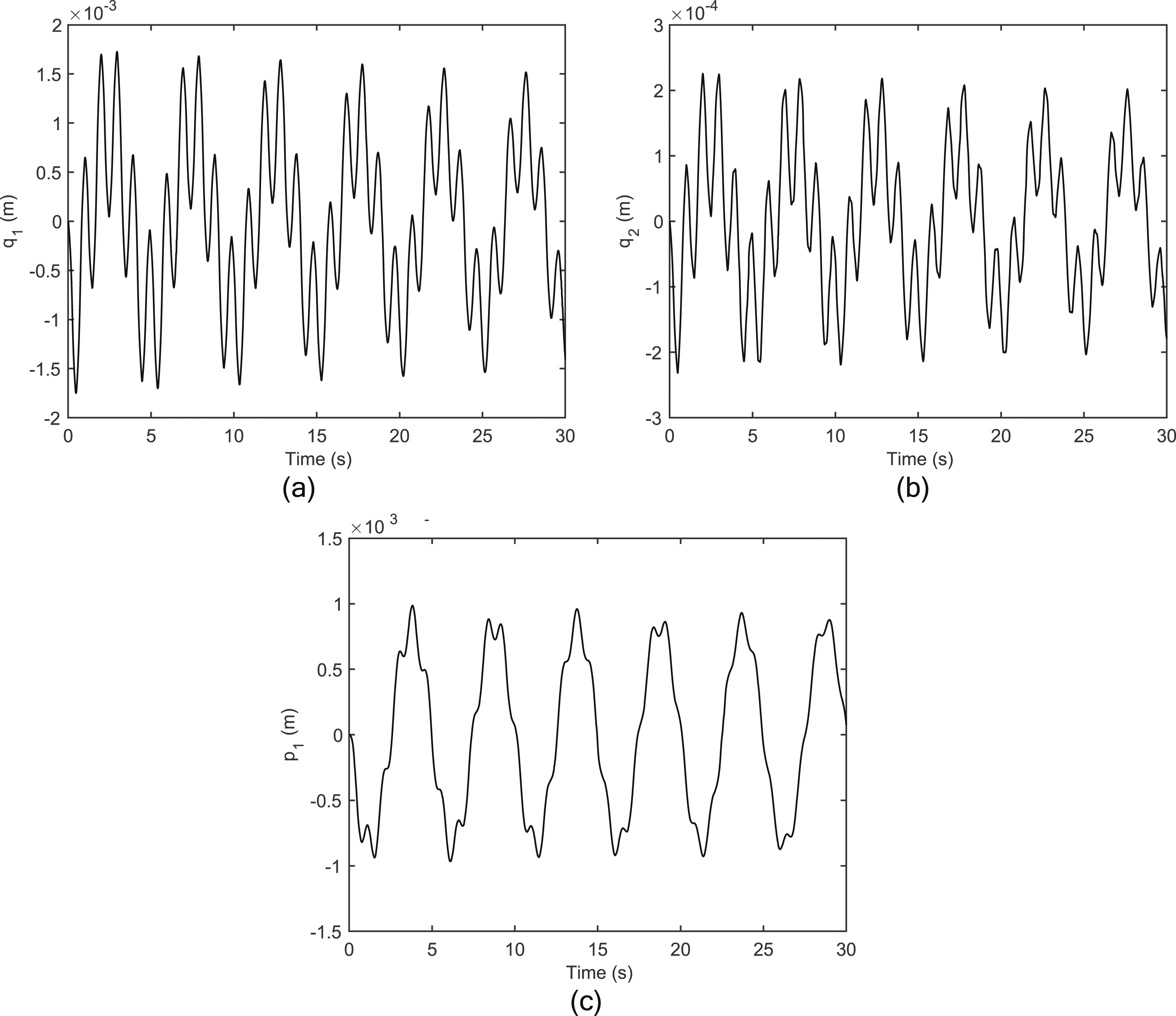
(a): amplitudes in non-resonant condition, (b): phase portraits in non-resonant condition, (c): amplitudes in the internal resonance condition using $a_{1-3}=0.5,{\theta }_{1-3}=0$ , (d): phase portraits in the internal resonance condition using $a_{1-3}=0.5,{\theta }_{1-3}=0$ , (e): amplitudes in the internal resonance condition using $a_{1-3}=0.6,{\theta }_{1-3}=0$ , (f): phase portraits in the internal resonance condition using $a_{1-3}=0.6,{\theta }_{1-3}=0$ .

Two sets of initial values, $a_{1-3}=0.5,{\theta }_{1-3}=0$ and $a_{1-3}=0.6,{\theta }_{1-3}=0$ are used to find the amplitudes in the case of internal resonance. First flapwise and edgewise vibrations are in synchronization as depicted in Figure 8(c). It is further noticed that there is an ongoing transfer of energy from first flapwise mode, first edgewise mode to the second mode associated with the flapwise direction as illustrated in Figures 8(c) and (e). As shown in Figures 8(c) and (e), even a slight disturbance in the initial state of motion can significantly alter the dynamic attributes of the blade.

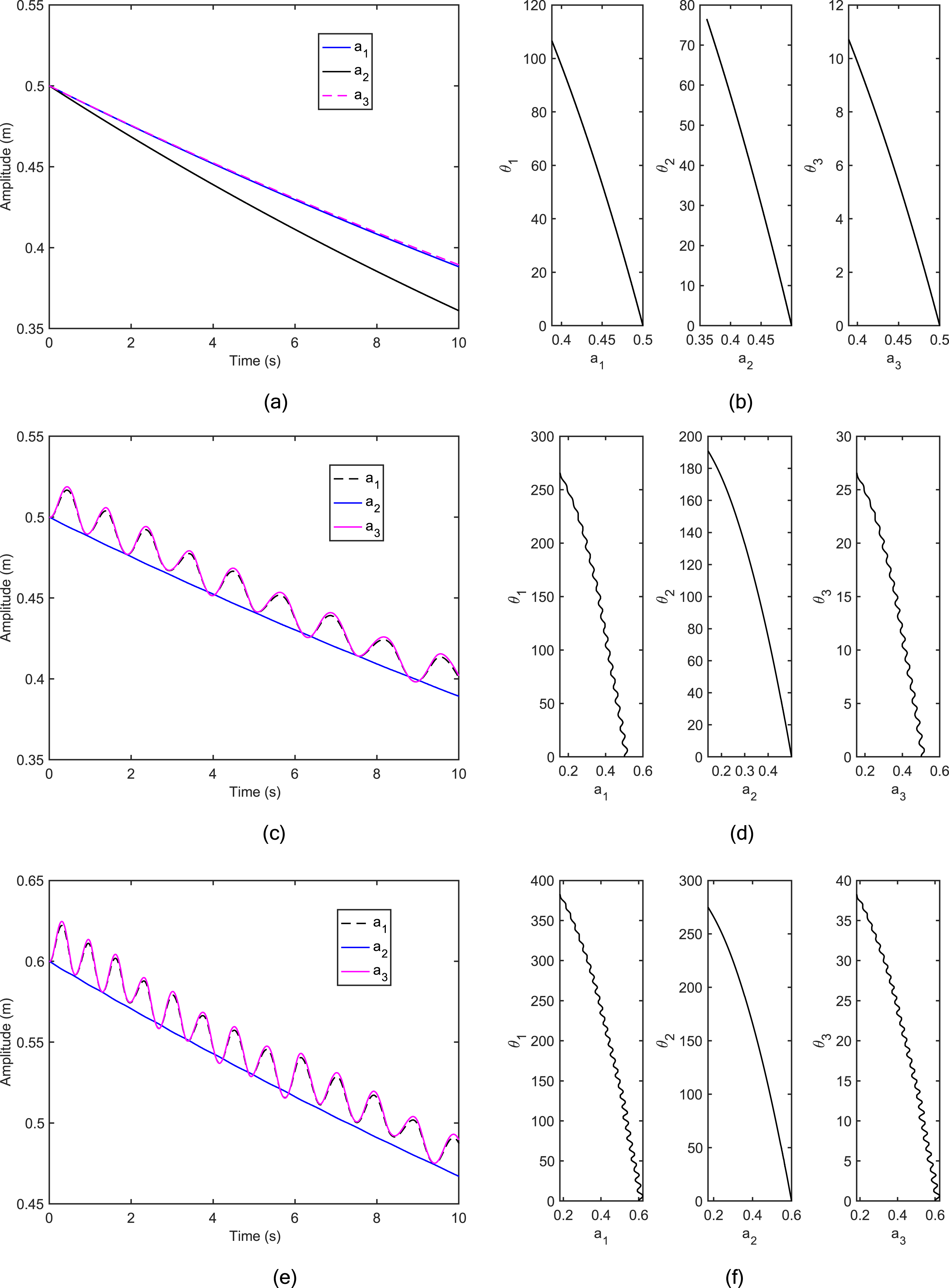
Using the initial values as $a_3=0.5,{\theta }_3=0$ , amplitude of oscillation $a_3$ and phase diagram in case of primary resonance are illustrated in Figures 9(a) and 9(b).

Figure 9.

(a): amplitude $a_3$ during primary resonance, (b): phase portrait during primary resonance, (c): amplitudes $a_1,a_2$ during combination resonance, (d): amplitude $a_3$ during combination resonance (e): phase portraits during combination resonance.

In the combined internal and primary resonance condition, amplitudes $a_{1-3}$ are computed by solving equations (61)–(66) using the initial values of $a_{1-3}=0.5$ , ${\theta }_{1-3}=0$ . The intensity of the first edgewise mode reaches its highest energy level as represented in Figure 9(d).

4.2. Steady-state responses under primary and combination resonances using multiple-scales method

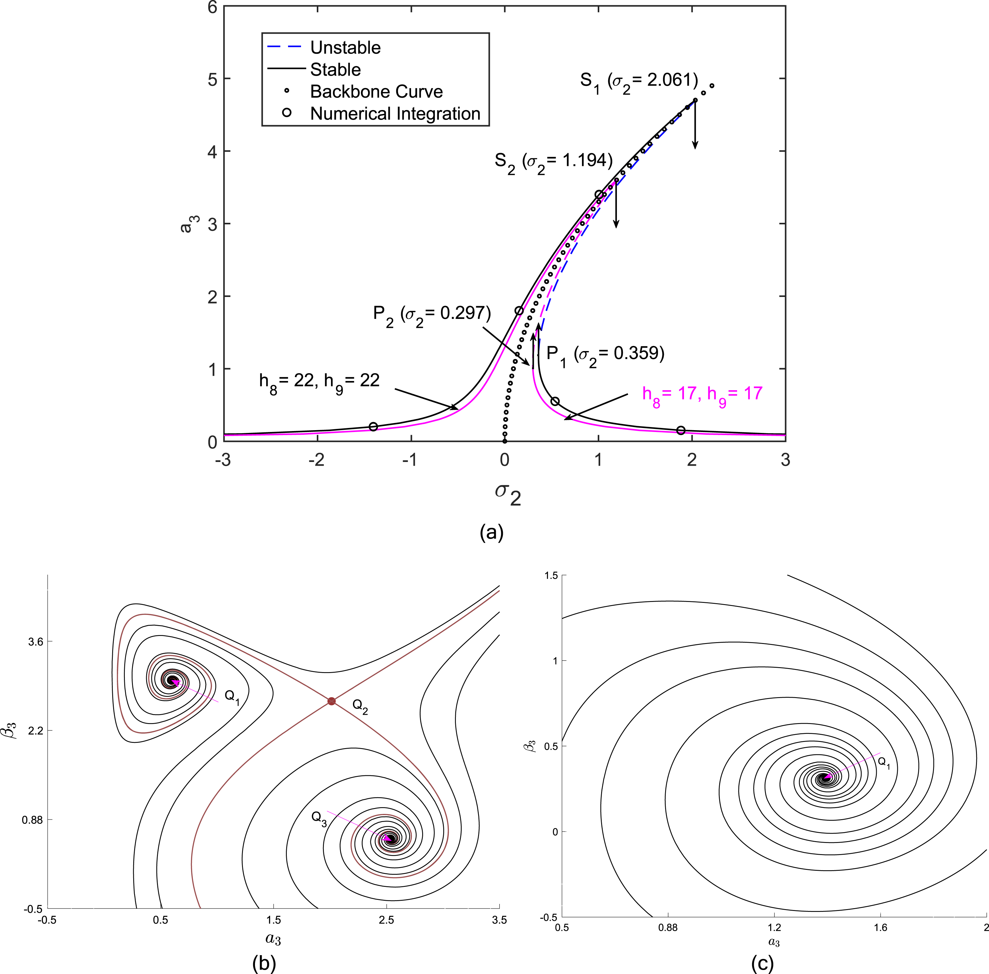
Once the initial transient response has been effectively dissipated, oscillation of the blade will enter a steady-state stage. We will analyze the effects of geometric nonlinearity and aerodynamic force on the steady-state responses for primary and combination resonances. Figure 10(a) depicted the first edgewise amplitude under primary resonance. Based on equation (60), the steady-state response is finely tuned to align with frequency of excitation. However, there exists a discrepancy in the phase between response and excitation, represented by $-{\beta }_3$ . The angle ${\beta }_3{=\sin }^{-1}\left(R_{32}{a}_3/{2R}_{37}\right)$ from equation (57), represents the phase shift of the response due to the presence of damping. Equation (59) demonstrates that the peak amplitude is determined by ${\left(a_3\right)}_p=\left(2R_{37}/R_{32}\right)$ , it remains unaffected by the value of $R_{33}$ , which plays a crucial role in the nonlinearity of the frequency-response curve. Figure 10(a) depicts that the cubic nonlinearity bends the curve to the right, this indicates that the blade behaves like hardening spring. As the amplitude of excitation of aerodynamic force grows, curve gradually bends away from ${\sigma }_2=0$ . Parabola ${\sigma }_2=\left(R_{33}/4R_{31}\right)a_3^2$ represents the locus of the peak amplitude, which is the backbone curve, shown by a dotted line in Figure 10(a).

Figure 10.

In the event of primary resonance (a): effect of aerodynamic force on first edge wise Amplitude $a_3$ , (b): phase portraits when ${\sigma }_2=0.51$ , (c): phase portraits when ${\sigma }_2=0$ .

An upward jump from point $P_1$ occurs for $a_3$ when ${\sigma }_2$ reaches a specific critical value and drops. Further, another downward jump happens from point $S_1$ with an accompanying decrease in $a_3$ when ${\sigma }_2$ increases to a certain value. Region of the curve between points $P_1$ and $S_1$ is unstable. Figures 10(b) and (c) depict the phase diagrams of first edgewise mode under primary resonance. For ${\sigma }_2=0$ , the phase diagram possesses only a single stable focus $\left(Q_1\right)$ . For ${\sigma }_2=0.51$ , there are two stable focus points $\left(Q_1\right)$ and $\left(Q_3\right)$ , and one saddle point $\left(Q_2\right)$ .

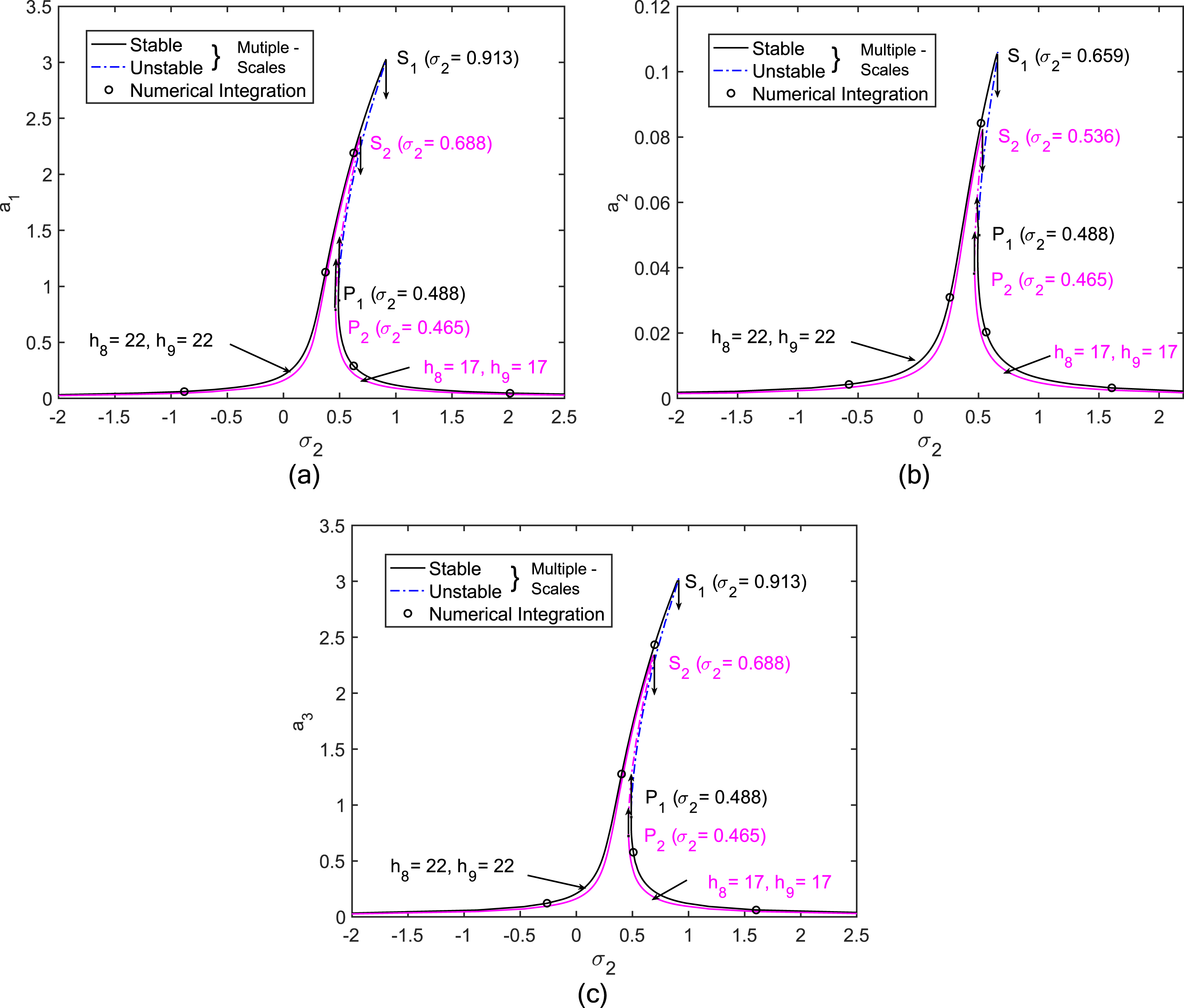
Although the excitation of the fundamental mode $\left(\mathrm{\Omega }={\omega }_1\right)$ does not generate substantial responses in the higher modes (Nayfeh and Mook, 1979). Therefore, the excitation of the higher mode $\left(\mathrm{\Omega }={\omega }_3\right)$ is used in this work. Figure 11 showcases the frequency-response curves under combination resonance. Once again, due to the presence of cubic nonlinearity, blade exhibits the hardening spring behavior. Furthermore, it has been discovered that a greater amplitude of excitation not only results in a more robust level of oscillation but also widens the region of instability. Amplitude $a_3$ under the combination resonance in Figure 11(c) is less than what it was during the primary resonance in Figure 10(a). This indicates that internal resonance serves as the means through which energy is transferred from one mode to other modes. This also implies that by adjusting the internal resonance of flapwise modes, it is possible to effectively stabilize the primary resonance of an unstable edgewise mode.

Figure 11.

In the event of combination resonance—effect of aerodynamic force on (a): first flapwise amplitude $a_1$ , (b): second flapwise amplitude $a_2$ , (c): first edge wise Amplitude $a_3$ .

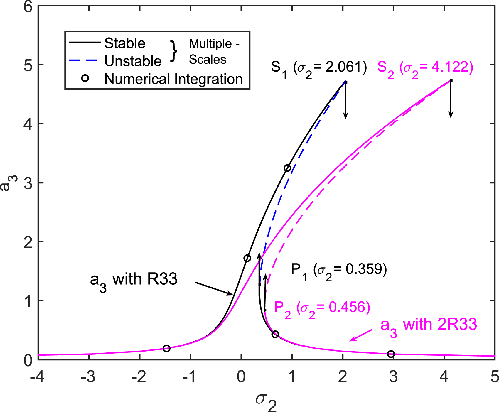
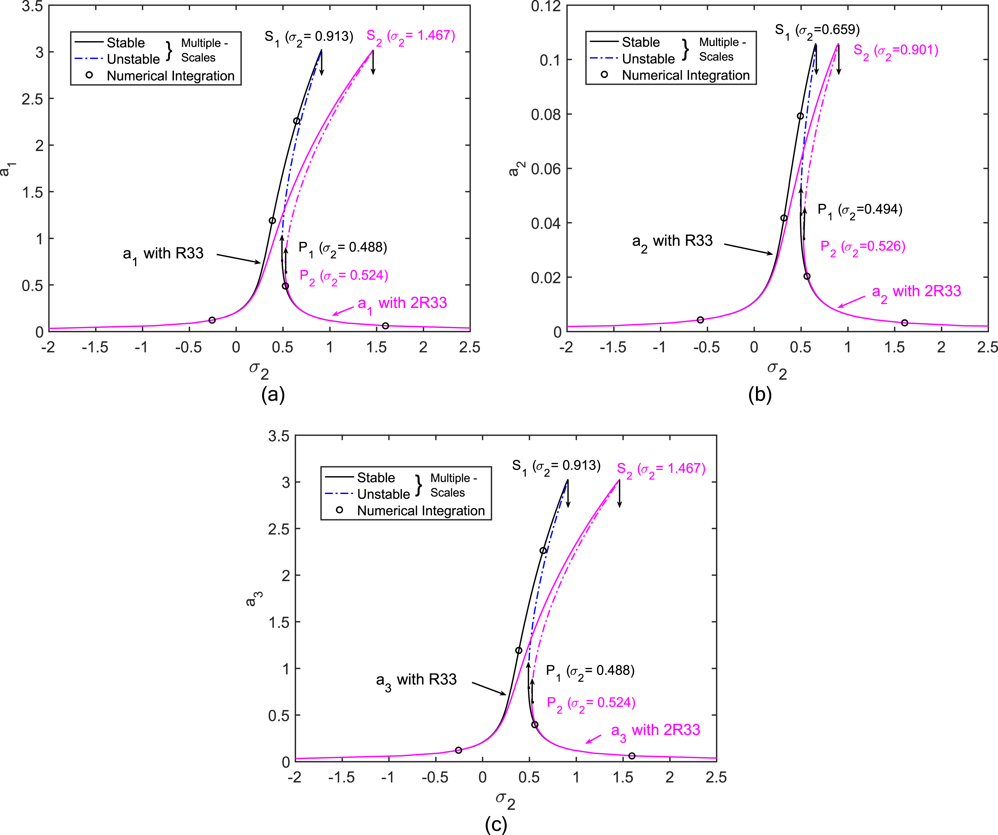
Figures 12 and 13 illustrate the impacts of geometric nonlinearity (coefficient $R_{33}$ ) under primary and combination resonances, respectively. For both the scenarios, greater tensile rigidity intensifies the influence of hardening behavior and broadens the unstable motion. Flapwise amplitudes have the potential to be amplified by increasing geometric nonlinearity, which sets them apart from edgewise amplitudes.

Figure 12.

Effect of geometrical nonlinearity on first edge wise amplitude $a_3$ for primary resonance.

Figure 13.

In the event of combination resonance—effect of geometrical nonlinearity on (a): first flapwise amplitude $a_1$ , (b): second flapwise amplitude $a_2$ , (c): first edge wise Amplitude $a_3$ .

4.3. Stability of steady-state responses

The stability can be determined by superimposing small perturbation on the singular points of equations (57) and (58) under primary resonance, by letting

$a_3=a_0+a_{31},{\hspace{0.17em}\beta }_3={\beta }_0+{\beta }_{31}$

(70)

where $a_{31}$ and ${\beta }_{31}$ are small compared to $a_0$ and ${\beta }_0$ . Substituting equation (70) into equations (57) and (58) and linearizing the resulting equations in $a_{31}$ and ${\beta }_{31}$ , we obtain

$a_{31}^{\prime }=\left(\frac{R_{32}}{R_{31}}\right)a_{31}+\left(\frac{2R_{37}}{R_{31}}\right)\left(\mathit{cos}\hspace{0.17em}{\beta }_0\right){\beta }_{31}$

(71)

${\beta }_{31}^{\prime }=\left[\left(\frac{R_{33}}{{2R}_{31}}\right)a_0+\left(\frac{{2R}_{37}}{R_{31}}\right)\left(\frac{1}{a_0^2}\right)\mathit{cos}\hspace{0.17em}{\beta }_0\right]a_{31}-\hspace{0.17em}\left(\frac{{2R}_{37}}{R_{31}}\right)\left(\frac{1}{a_0}\right)\left(\mathit{sin}\hspace{0.17em}{\beta }_0\right){\beta }_{31}$

(72)

We seek a solution for equations (71) and (72) in the form

$a_{31}=a_{10}{e}^{\lambda t_1},{\hspace{0.17em}\beta }_{31}={\beta }_{10}{e}^{\lambda t_1}$

(73)

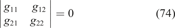
where $a_{31},{\beta }_{10}$ and $\lambda$ are constants. Hence the stability of the steady-state motions depends on the eigenvalues of the coefficient matrix on the right-hand side of equations (71) and (72) as

$\left|\begin{array}{ll}{g}_{11}& {\hspace{0.17em}g}_{12}\\ g_{21}& g_{22}\end{array}\right|=0$

(74)

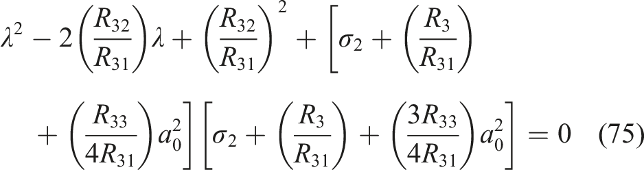
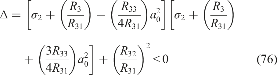
The coefficients $g_{11},{\hspace{0.17em}g}_{12},g_{21}$ and $g_{22}$ of equation (74) are defined in Appendix 3. Expanding equation (74) yields

${{\lambda }^2-2\left(\frac{R_{32}}{R_{31}}\right)\lambda +\left(\frac{R_{32}}{R_{31}}\right)}^2+\left[{\sigma }_2+\left(\frac{R_3}{R_{31}}\right)+\left(\frac{R_{33}}{{4R}_{31}}\right)a_0^2\right]\left[{\sigma }_2+\left(\frac{R_3}{R_{31}}\right)+\left(\frac{3R_{33}}{{4R}_{31}}\right)a_0^2\right]=0$

(75)

Thus, the steady-state motions are unstable when

$∆=\left[{\sigma }_2+\left(\frac{R_3}{R_{31}}\right)+\left(\frac{R_{33}}{{4R}_{31}}\right)a_0^2\right]\left[{\sigma }_2+\left(\frac{R_3}{R_{31}}\right)+\left(\frac{3R_{33}}{{4R}_{31}}\right)a_0^2\right]+{\left(\frac{R_{32}}{R_{31}}\right)}^2<0$

(76)

The condition of the equation (76) corresponds to the portion between points ${\hspace{0.17em}P}_1\left({\sigma }_2=0.359\right)$ and ${\hspace{0.17em}S}_1\left({\sigma }_2=2.061\right)$ when $h_8=h_9=22$ in Figures 10(a) and 12, because these points correspond to $∆=0$ . The range of detuning parameter ${\sigma }_2$ that corresponds to unstable steady-state motions under the primary resonance is ${\sigma }_2\hspace{0.17em}ϵ\hspace{0.17em}\left(0.297,1.194\right)$ when $h_8=h_9=17$ based on Figure 10(a). Since we have complex eigenvalues with real part smaller than zero after solving the Jacobian of equation (74), hence we get a stable focus $\left(Q_1\right)$ as shown in phase diagram (Figure 10(c)).

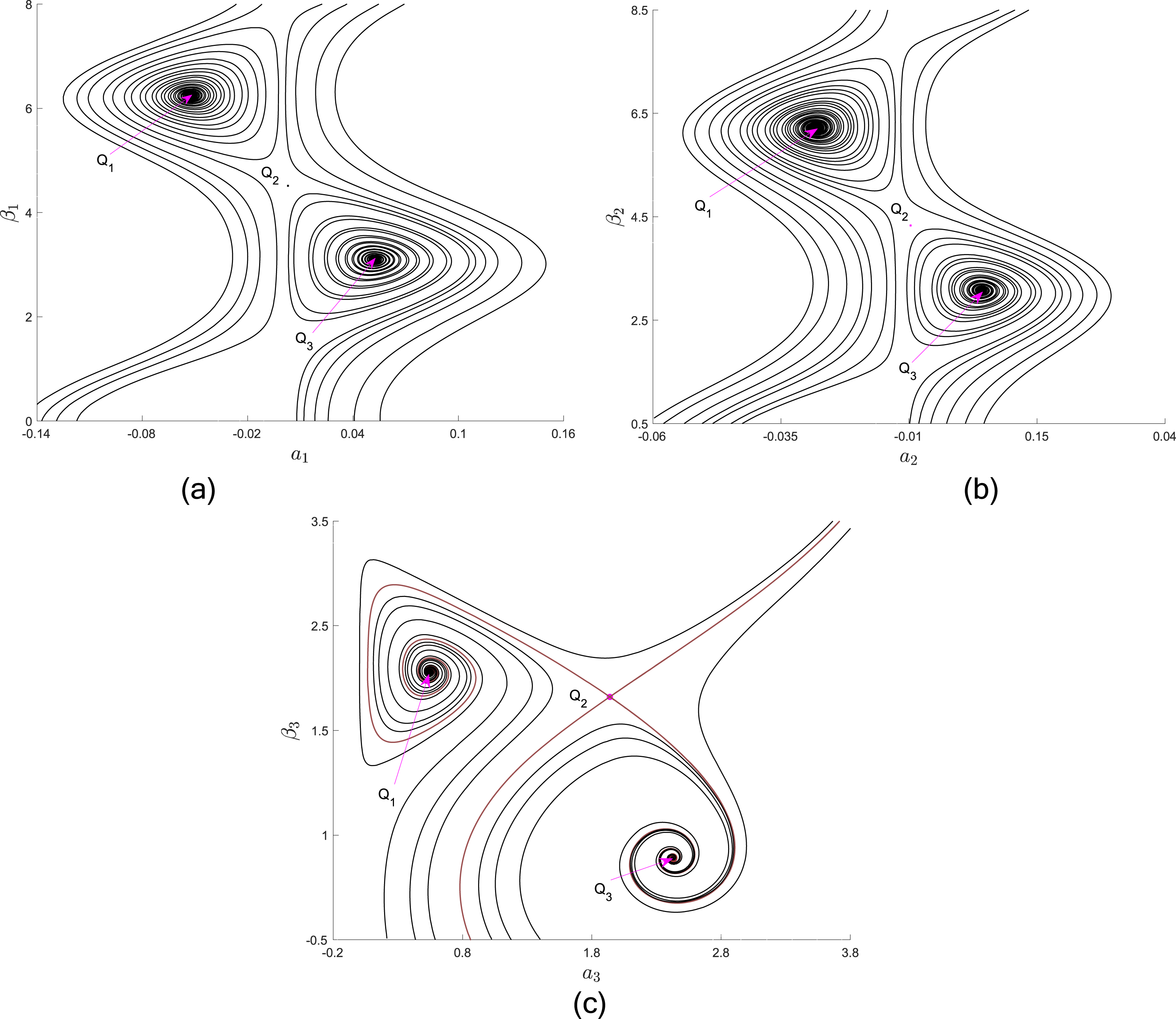
The unstable steady-state motions under combination resonance are found by using the same methodology of equations (70)–(76) for primary resonance. In the combination resonance scenario while considering the effects of geometric nonlinearity, the unstable motions exist in the regions ${\sigma }_2\hspace{0.17em}ϵ\hspace{0.17em}\left(0.524,1.467\right)$ when ${2R}_{33}$ rather than ${\sigma }_2\hspace{0.17em}ϵ\hspace{0.17em}\left(0.488,0.913\right)$ when $R_{33}$ for $a_1$ and $a_3$ based on Figure 13. For $a_2$ , the unstable regions are ${\sigma }_2\hspace{0.17em}ϵ\hspace{0.17em}\left(0.526,0.901\right)$ when ${2R}_{33}$ and ${\sigma }_2\hspace{0.17em}ϵ\hspace{0.17em}\left(0.494,0.659\right)$ when $R_{33}$ . Once again, we obtained complex eigenvalues having negative real part, which indicates a stable focus $\left(Q_3\right)$ as depicted in Figure 14.

Figure 14.

Phase portraits due to combination resonance when ${\sigma }_2=0.51$ (a): for first flapwise mode (b): for second flapwise mode, (c): for first edgewise mode of vibration.

5. Conclusion

A nonlinear dynamic model was derived to investigate the HAWT blade vibrations in two principal axes, also including the geometric nonlinearities of curvature and inertia terms. Three coupled equations were obtained, one in edgewise direction and two in flapwise direction. Transient and steady-state responses of a reference NREL 5-MW HAWT blade were studied. An important conclusion is that the dominant modes of vibration are first edgewise and first flapwise, while second flapwise mode of vibration is considerably less significant for the coupled modal equations in vibration analysis. The results demonstrated that energy transfers occur between different modes through internal and combination resonances. In the scenario of combined resonance, exchange of energy between the modes exceeded that of the internal resonance situation.

Based on the frequency response results, it was demonstrated that geometric nonlinearity amplification leads to a heightened energy transfer via internally resonating modes. As the frequency gradually increases and diminishes, there can be hysteresis and jump phenomena resulting in substantial distortions. In the event of combined resonance, the frequency response initially rises and subsequently declines as the inflow ratio rises. This phenomenon arises from the collective effect of aerodynamic force and damping. Further comprehensive dynamic modeling is currently in progress to incorporate the coupled vibrations of edgewise-flapwise-torsional motions, with the aim of fully grasping the dynamics of the system.