
Abstract
Major problems can occur when liquid sloshes in a tank, such as in liquid storage tanks during an earthquake, and this is an important engineering problem to address. To analyze this phenomenon, the finite-element method is generally used but involves many degrees of freedom when the tank is large. In this paper, a nonlinear numerical model with relatively few degrees of freedom is established for vertical and horizontal two-dimensional nonlinear sloshing in a rectangular tank excited horizontally. In addition, a method is proposed for reducing the number of degrees of freedom in the two-dimensional model. The natural frequencies, modes, and frequency responses are then compared among the concentrated mass model, theoretical calculations, and experimental results. Good agreement was achieved among them, thus demonstrating the validity of the model.
Introduction
Major problems can occur when liquid sloshes in a tank. For instance, the 2003 Tokachi-oki earthquake in Japan damaged a large tank storing oil at an industrial facility, causing a fire (Hatayama, 2008). Numerical simulations have been attempted by many researchers to understand sloshing behavior.
In analytical research, Moiseev (1958) presented a generalized theory for determining nonlinear sloshing behavior in a tank of arbitrary shape by using a perturbation method, and Faltinsen (1974) applied Moiseev’s theory to sloshing phenomena in a rectangular tank. Hayama et al. (1983) derived a similar theory that considers nonlinear free-surface conditions not considered by Moiseev, and they compared numerical results from their theory with the results of experiments involving a rectangular tank. With regard to the multimodal method, Faltinsen et al. (2000) and Faltinsen and Timokha (2002) derived a multimodal method based on two-dimensional potential theory and used it to simulate sloshing phenomena in a rectangular tank at shallow and intermediate water depths. However, the aforementioned perturbation and multimodal methods, which involve closed-form solutions, cannot be applied to tanks with complex shapes because only rectangular and cylindrical tanks yield linear theoretical solutions (Komatsu, 1958). Komatsu (1958) used the multimodal method to derive a nonlinear ordinary differential equation for sloshing and then solved it using the perturbation method for application to tanks of arbitrary shape. Love and Tait (2011, 2015) used the multimodal method to derive a nonlinear ordinary differential equation, and they solved it by numerical integration for application to flat-bottom tanks with arbitrary three-dimensional geometries. However, in the methods used by Komatsu (1958) and Love and Tait (2011, 2015), the mode shapes must be obtained in advance by using an approach such as the finite-element method (Love and Tait, 2011).
Regarding numerical analysis methods based on potential flow theory, Ikegawa (2002) derived a functional considering nonlinear free-surface boundary conditions and applied it to a finite-element method to solve nonlinear sloshing problems in a two-dimensional rectangular tank excited horizontally. Nakayama and Washizu (1980) extended Ikegawa’s method and analyzed the problem of a rectangular tank subjected to forced pitching oscillation. Wu et al. (1998) developed a finite-element model by using the Galerkin method to analyze sloshing in three-dimensional rectangular tanks. Nagashima (2009) applied the level-set extended finite-element method to sloshing in a rigid tank; in that approach, a finite-element mesh covers the entire domain in the tank including the air domain, and a signed distance function is defined to represent the distance from the free surface. In another approach, Faltinsen (1978) and Nakatama and Washizu (1981) developed a boundary-element method based on potential flow theory to solve nonlinear sloshing problems in a two-dimensional rectangular tank. However, the finite-element method and the boundary-element method involves many degrees of freedom when the tank is large.
To avoid the problem of high computational costs for FEM, an equivalent mechanical model consisting of masses, springs (or pendulums), and dashpots is often used. The model is derived so that natural frequencies and force acting on the side wall correspond to other solution. Linear mechanical models have been introduced for sloshing in a rectangular tank (Graham and Rodriguez, 1952) and in a cylindrical tank (Abramson et al., 1961) by using theoretical solutions of potential theory. Bauer (1966) developed nonlinear mechanical models for a cylindrical tank by using theoretical equations. However, there is no theoretical solution for tanks other than rectangular and cylindrical ones. For other shapes of tanks, Housner (1957) proposed a method for generating an equivalent mechanical model of an arbitrarily shaped tank by dividing elements in the horizontal and vertical directions. However, this model is linear and cannot calculate variations in the water level accurately (Kaneko, 2016). Methods to determine the linear mechanical model parameters for arbitrary tank shapes were developed by using experimental data (Sumner, 1965) or FEM results (Dorosos et al., 2008). Godderidge et al. (2012) developed a nonlinear mechanical model by using computational fluid dynamics simulation. However, for mechanical models other than cylindrical and rectangular tanks, it is necessary to perform experiments and numerical calculations in advance.
The ultimate aim of the work reported here is to establish a practical analytical model comprising one-dimensional masses and springs for analyzing nonlinear sloshing phenomena in a tank of arbitrary shape without the need to perform experiments and numerical calculations in advance. In this paper, we propose a model of a rectangular tank as a first step. In the process of deriving the model, it is not necessary to perform numerical calculations in advance to obtain the mode shapes or any other information for the mechanical model; however, as reported herein, experiments and numerical calculations with the proposed model must be performed in advance to identify the damping parameter. In previous studies, we proposed a one-dimensional concentrated mass model to analyze large-amplitude nonlinear sloshing phenomena in a rectangular tank containing shallow liquid (Ishikawa et al., 2016), where shallow is defined as a water depth that is less than one-fifth of the wavelength.
Herein, we propose a two-dimensional concentrated mass model to analyze the nonlinear sloshing phenomena to enable analysis of not only nonlinear shallow-water wave conditions but also nonlinear deep-water wave conditions. In this model, a method is proposed to transform the two-dimensional model into a one-dimensional model. As a first step toward arbitrarily shaped models, we propose the model for a rectangular tank. To validate the two-dimensional and reduced-DOF models, we compare the linear natural frequencies of the concentrated mass model with the corresponding theoretical values for a rectangular tank. To validate the model in a nonlinear region, we report on an experiment involving a rectangular tank and compare its results with the numerical ones.
Concentrated mass model
We consider two-dimensional nonlinear sloshing of liquid in a rigid rectangular tank excited horizontally, as shown in Figure 1(a). We assume that the liquid is incompressible with no surface tension and oscillates at amplitudes that are insufficient to cause wave breaking. The coordinate system is as shown in Figure 1. The liquid has horizontal length L
x
and equilibrium depth L
z
and is divided into N
x
and N
z
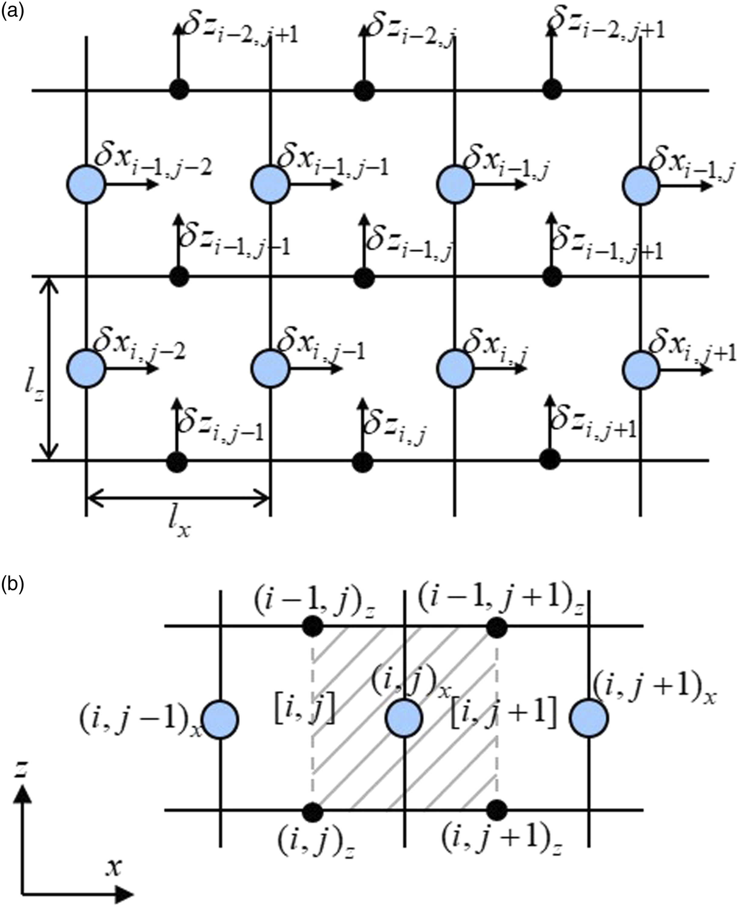
uniform elements in the x and z directions, respectively (Figures 1(b) and 2(a)); the element lengths are l
x
and l
z
in the x and z directions, respectively. The width of the tank in the y direction is taken as the unit length. Mass is concentrated on the centers of the right and left sides of each element, and the mass points are indexed as (i, j)
x
. Considering the mass of liquid in the shaded area in Figure 2(b), the mass m at each mass point is Sloshing phenomena in a rectangular tank. (a) Liquid in a rectangular tank. (b) elements and mass points. Elements, mass points in x direction, and z nodal points. (a) Displacements of mass points and z nodal points. (b) Number of elements, mass points, and z nodal points.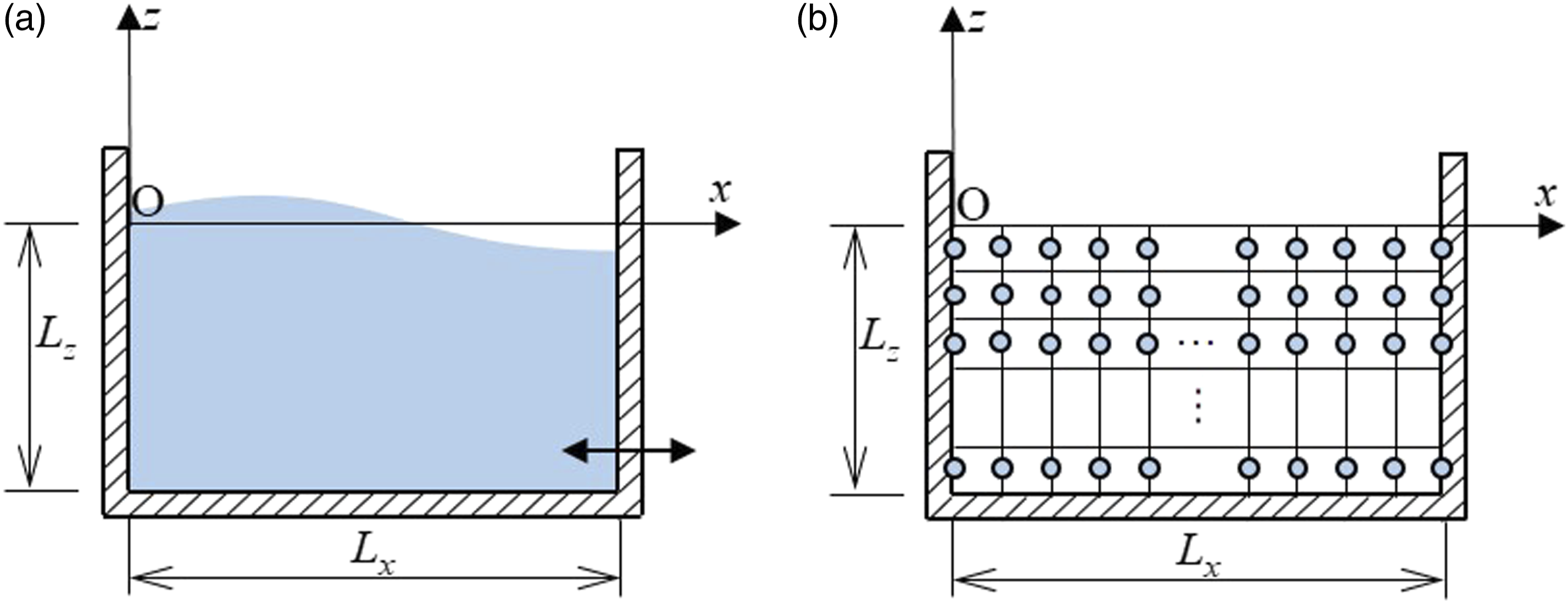

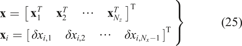
Connecting nonlinear springs
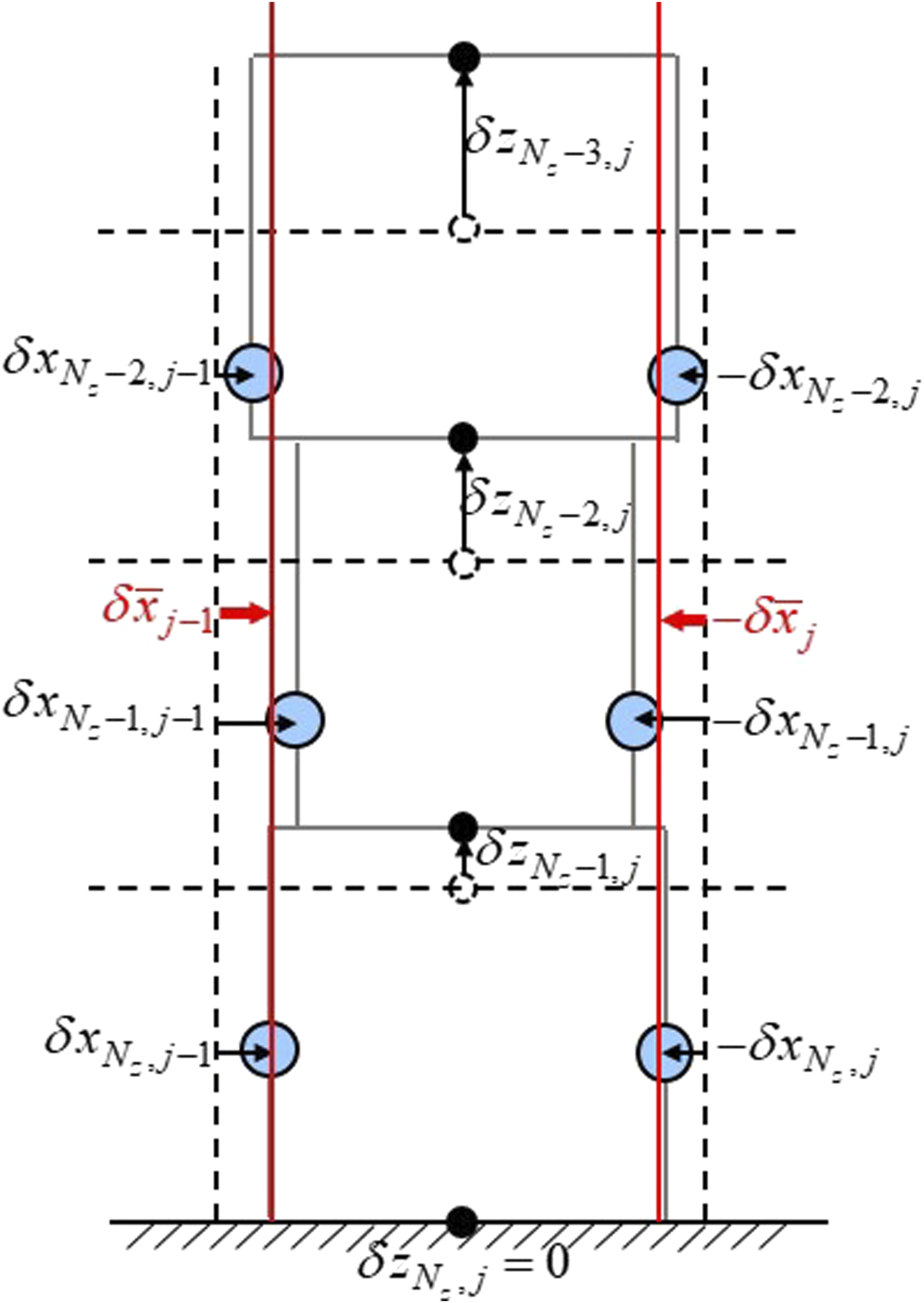
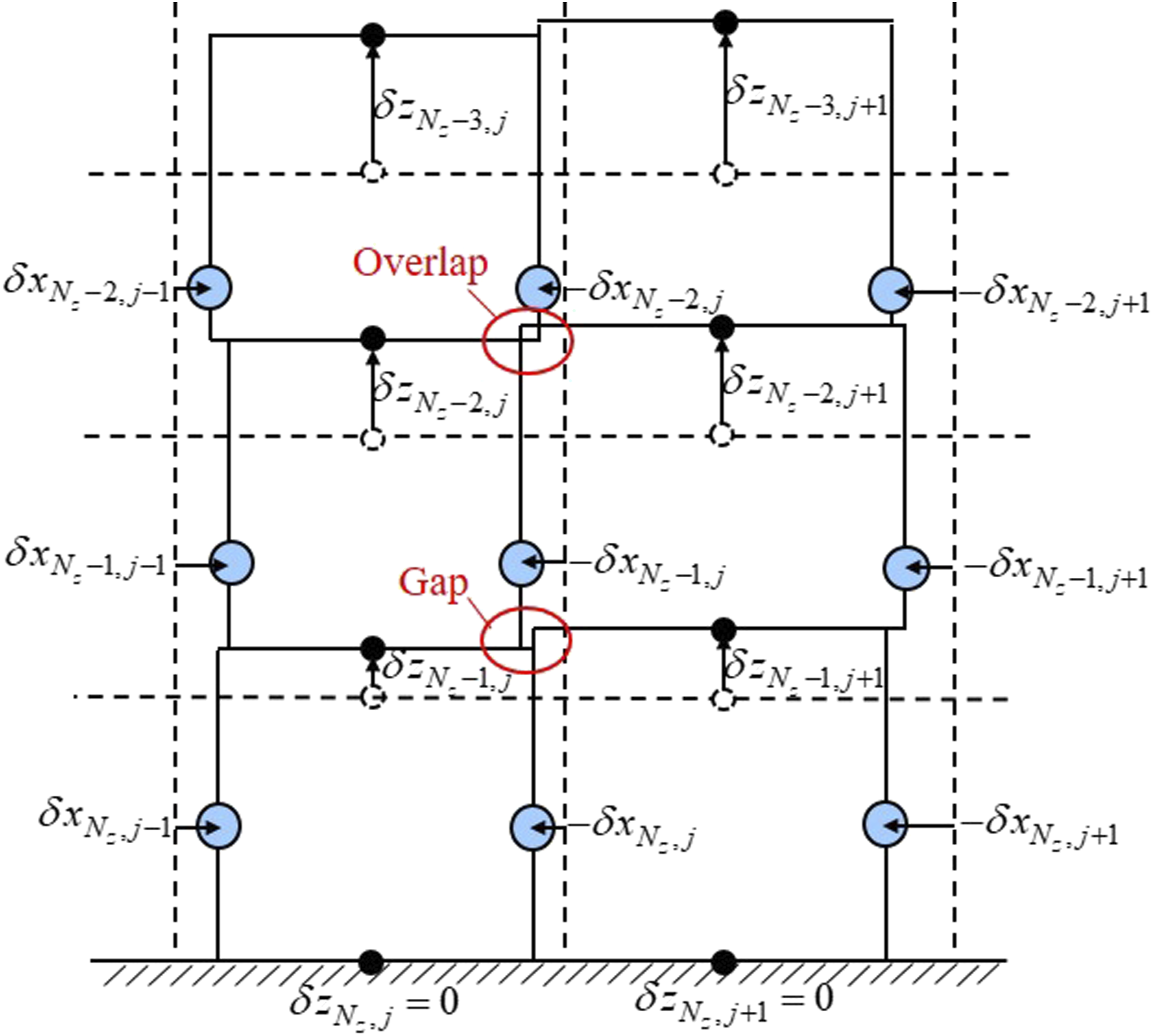
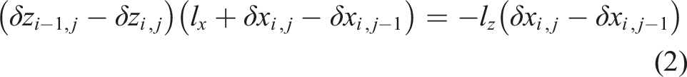
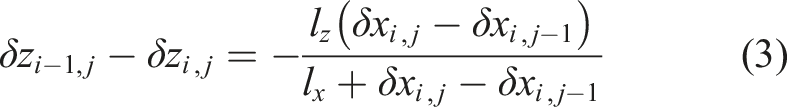
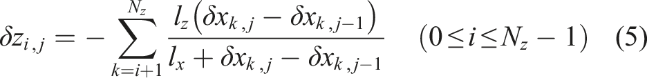
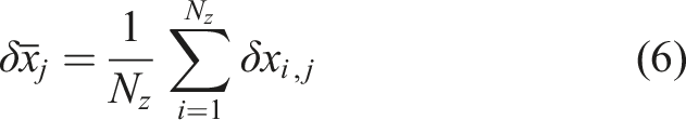
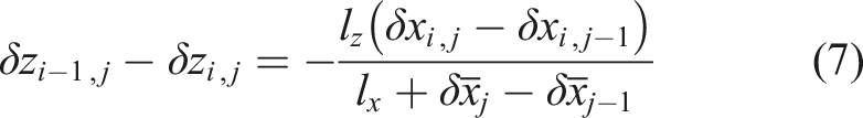
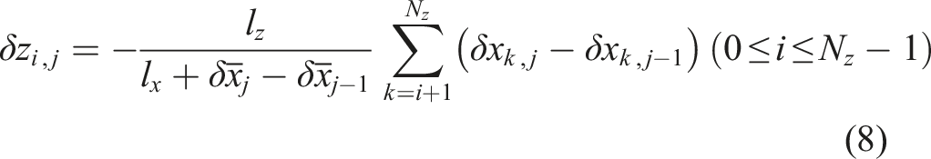
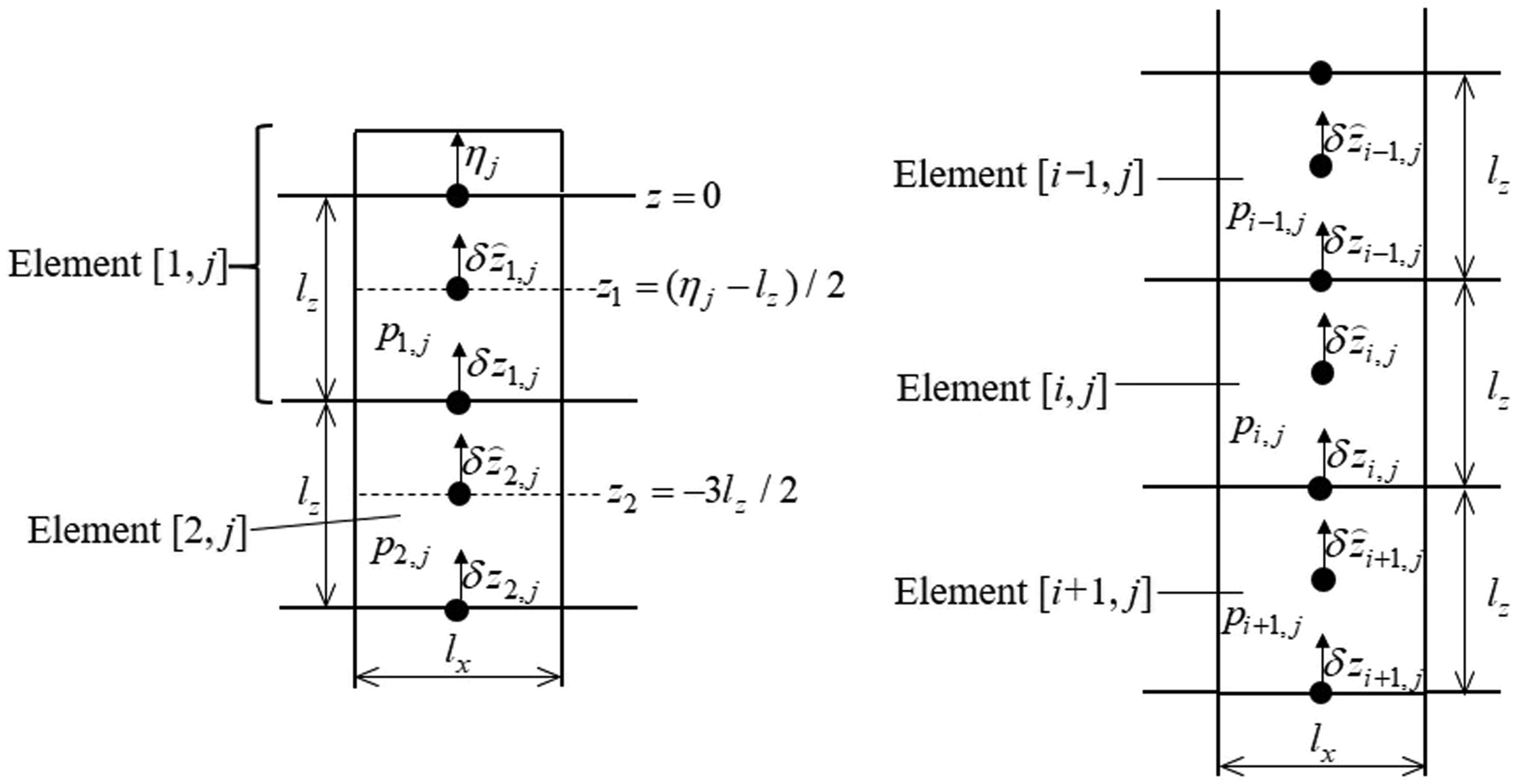
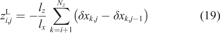
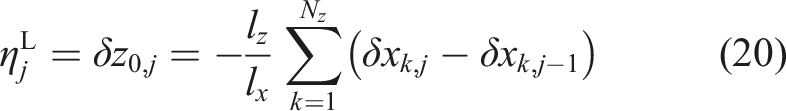
The nonlinear restoring forces acting on the mass points are derived from the hydrostatic pressure caused by the vertical displacement of the liquid surface and the hydrodynamic pressure caused by the vertical acceleration of the liquid. First, we derive the relationship between the displacement δxi, j of the mass points and the displacement δzi, j of the z nodal points. Because the liquid is incompressible, we assume that the z nodal points move while keeping the volume of each element in an arbitrary column j constant when the masses move, as shown Figure 3. From these relations, we obtain Deformation of element [i, j]. (a) Before deformation. (b) After deformation. Deformation of element from the bottom. Overlap and gap among elements.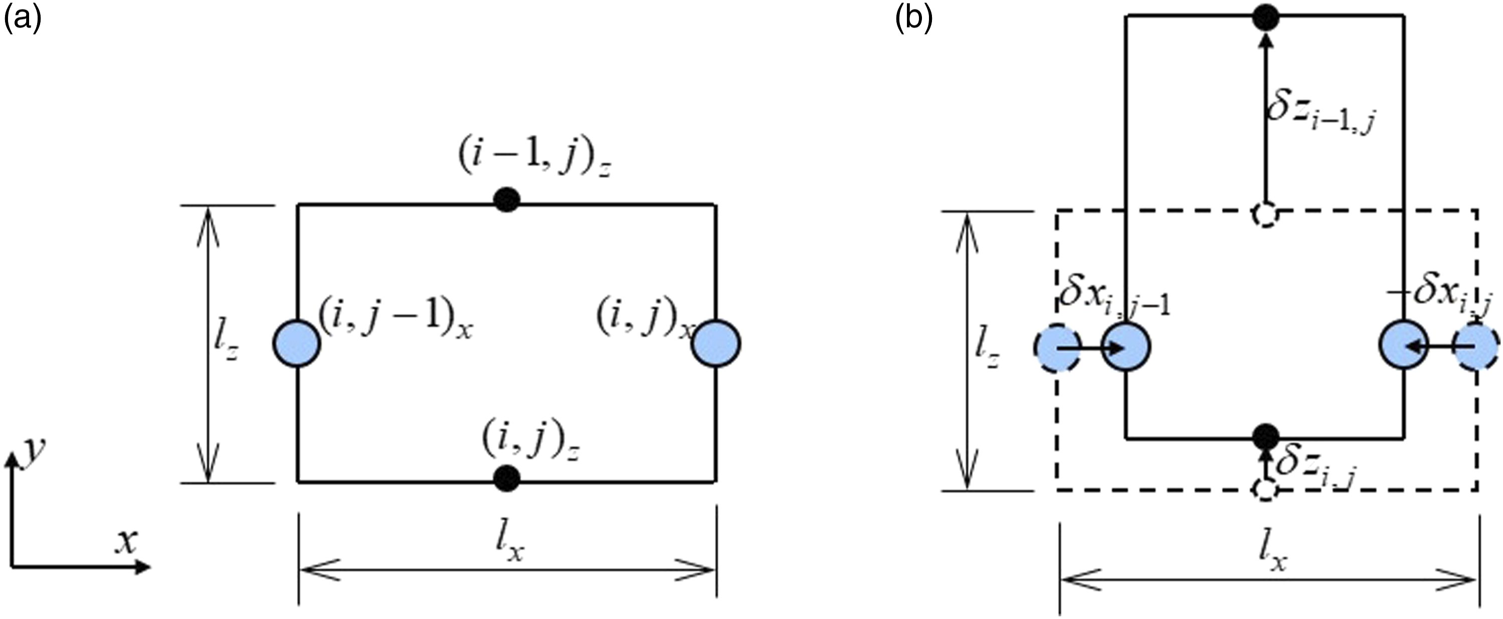

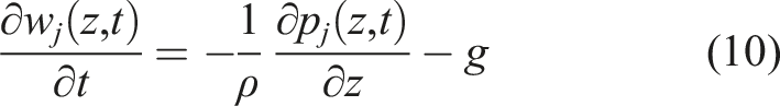
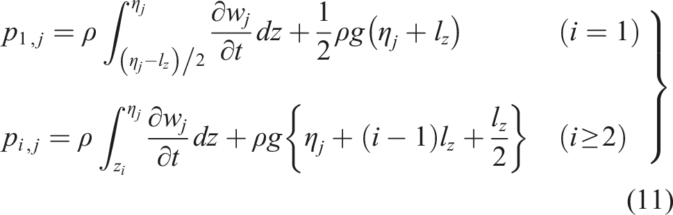
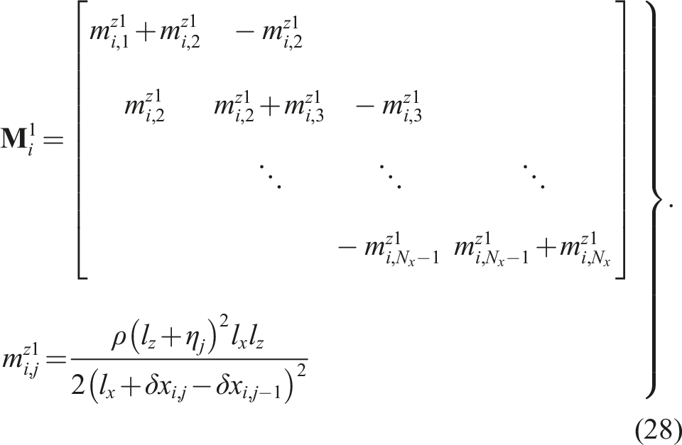
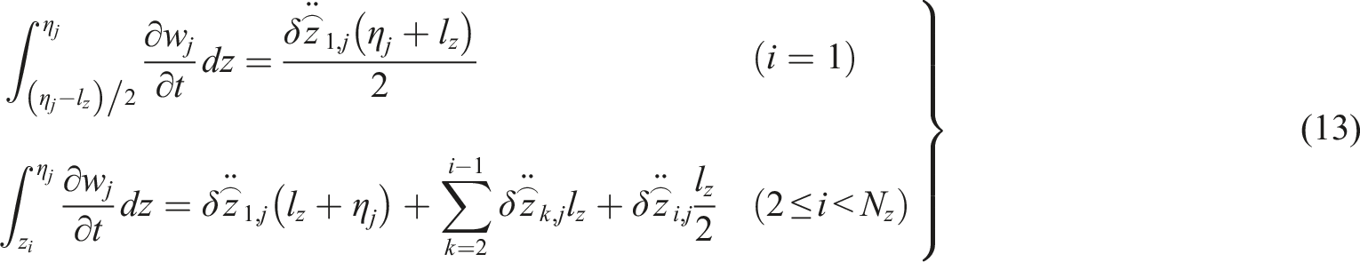
Second, we derive the pressure pi, j in element [i, j]. In the area of column j in Figure 6(a), Euler’s equation in the vertical direction is written as Control volume and interval of integration. (a) Control volume at column j. (b) Interval of integration. Acceleration of each element. (a) Around element [1, j]. (b) Around element [i, j].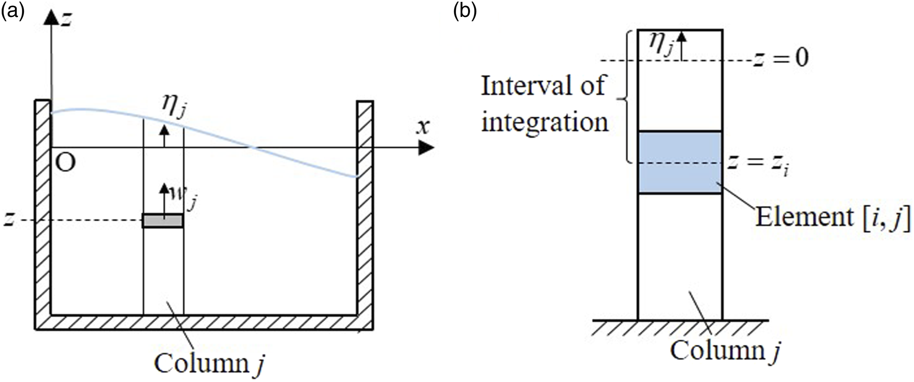
Third, we derive the restoring force acting on mass point (i, j)
x
from pressure pi, j. Assuming that
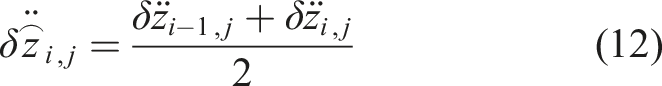
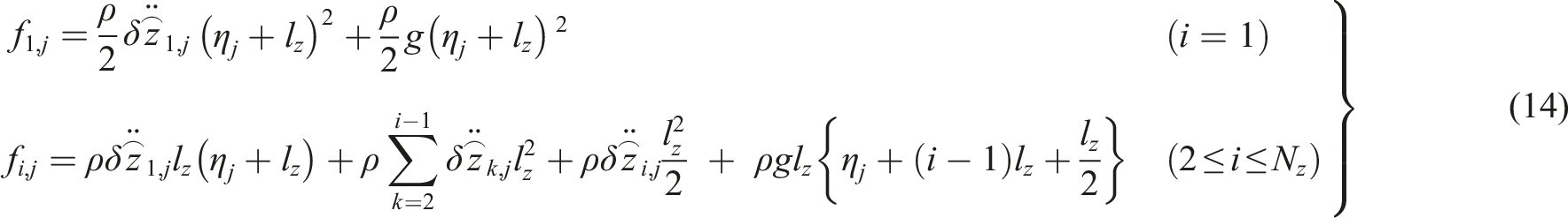
Multiplying pi, j in equation (11) by the vertical element length l
z
and using equation (13), the force fi, j acting on mass point (i, j)
x
becomes
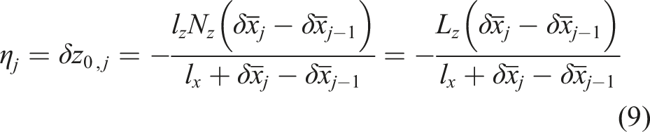
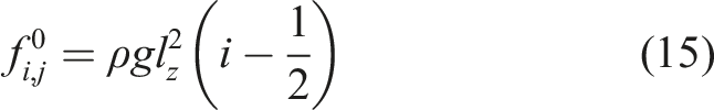
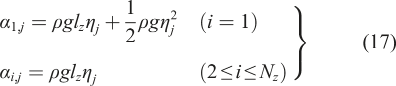
Herein, we assume that the vertical length of the top elements (i = 1) is (η
j
+ l
z
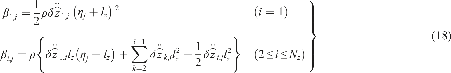
) when the liquid level changes. In the equilibrium state, the vertical displacement and the acceleration of the liquid surface are zero; therefore, the force

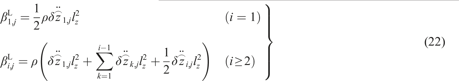
Linearizing equations (7), (9), (17), and (18), we obtain

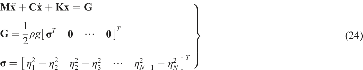
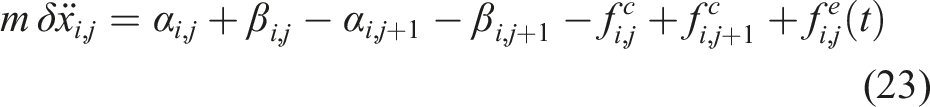
Equations of motion
The equation of motion of mass point (i, j)
x
is expressed as follows by considering the restoring forces acting from elements [i, j] and [i, j+1] (Figure 2(b))
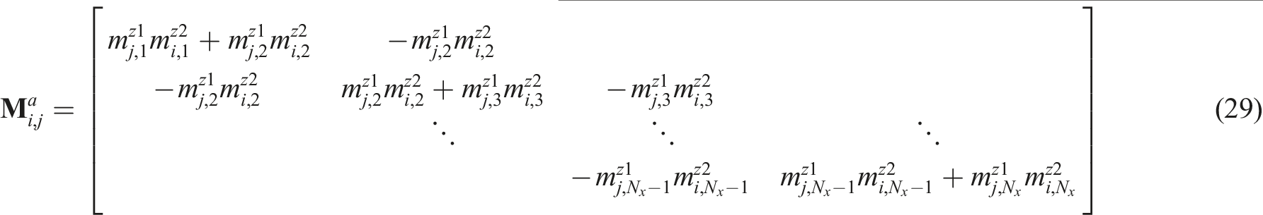
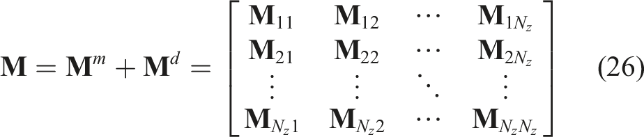
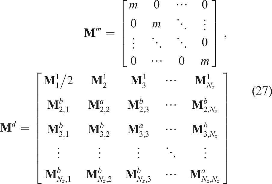
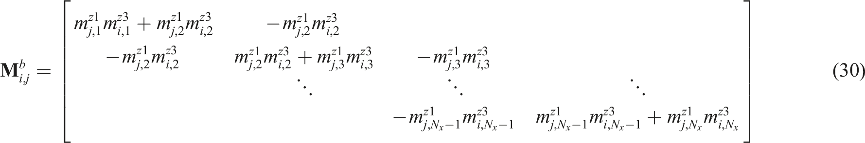
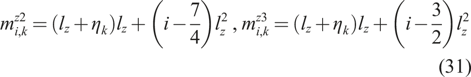
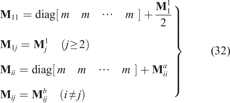
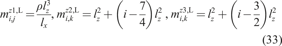
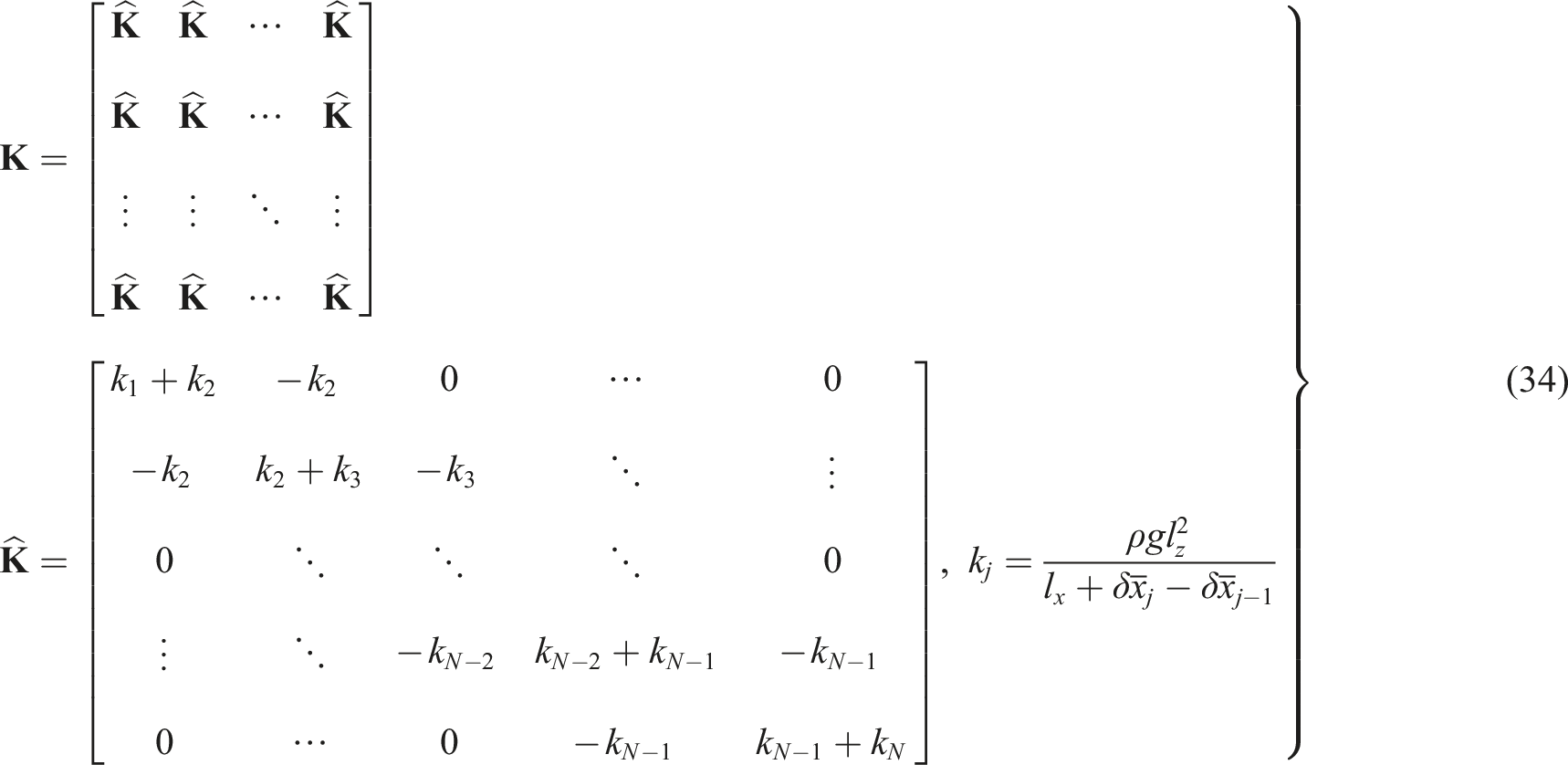
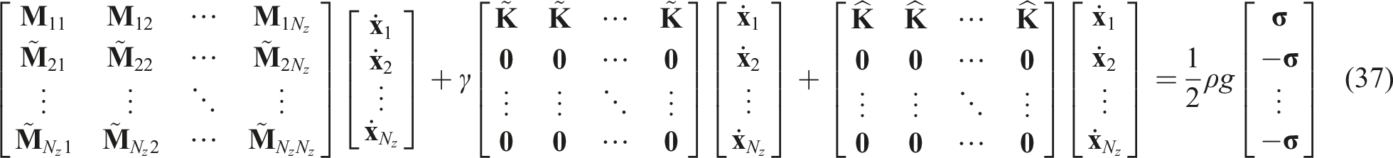
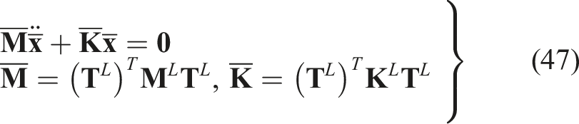
From equations (28), (31), and (34), the mass and stiffness matrices contain displacements.
where
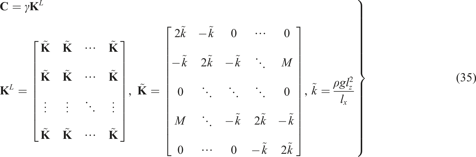
In addition, the damping matrix
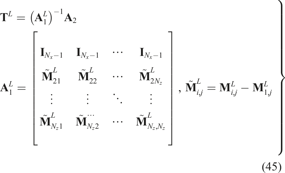
Reducing the number of degrees of freedom
In the model proposed in the section Concentrated Mass Model, the elements are divided vertically to consider the vertical velocity distribution, but, consequently, the model has an unnecessarily high number of DOFs, with zero-frequency eigenvalues being generated. In this section, we propose a way to reduce the number of DOFs of the concentrated mass model, as shown in Figure 8. Reducing the number of degrees of freedom (DOFs). (a) Two-dimensional model. (b) Reduced-DOF model.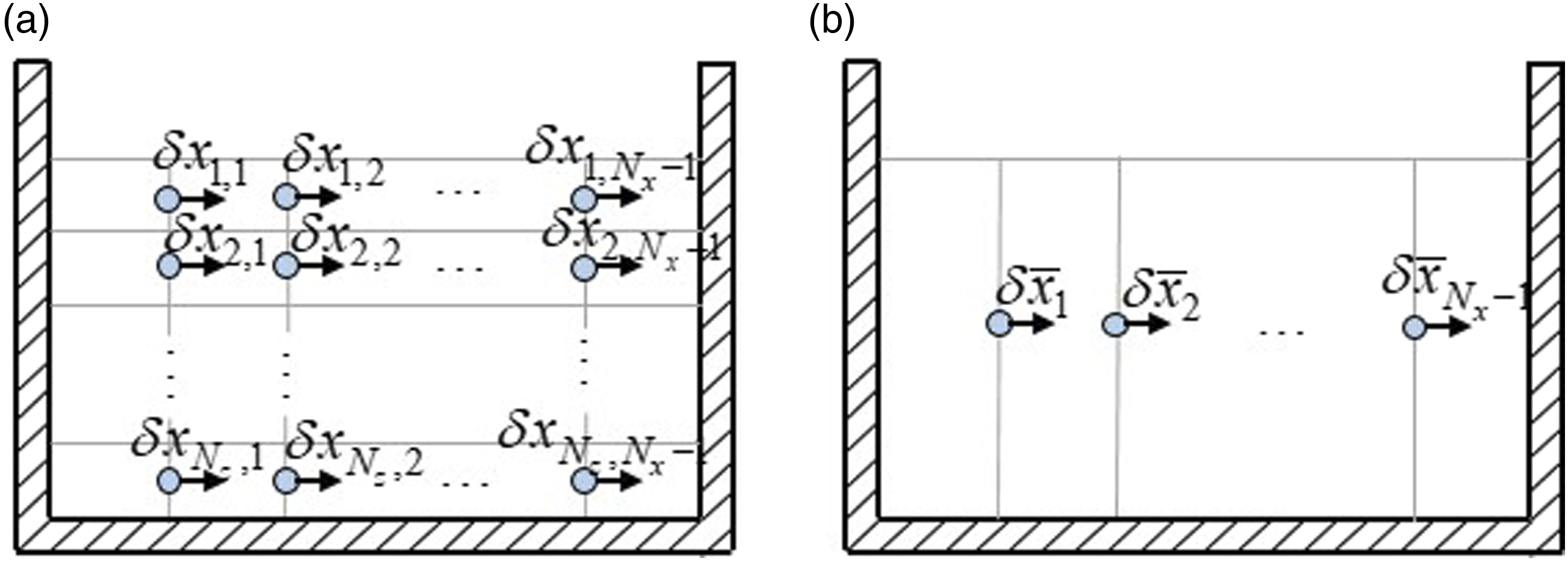
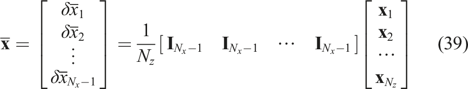
Using equations (26), (34), and (35), the equations of motion in equations (24) are rewritten as
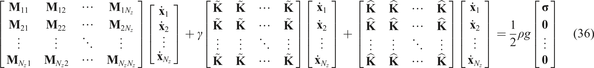
Here, the matrices

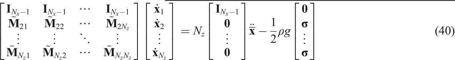
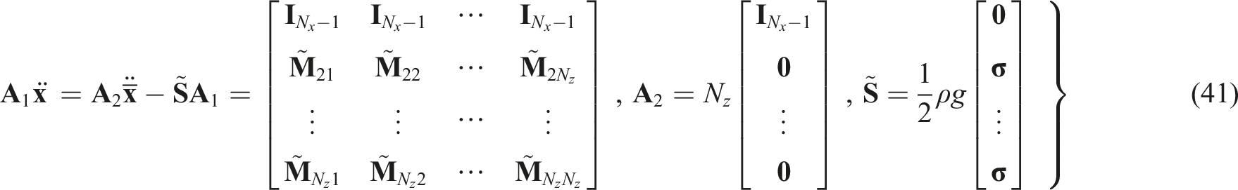
Multiplying
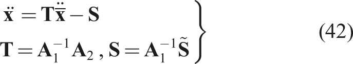
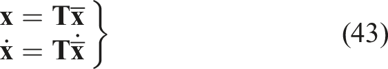
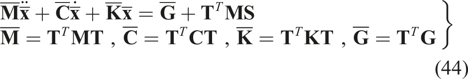
However, the transformation matrix
In the case of shallow water waves, the elements do not need to be divided vertically in a two-dimensional model because the velocity distribution is constant vertically (Ishikawa et al., 2016). The shallow water model due to Lepelletier and Raichlen (1988) involves one-dimensional equations using the average flow velocity, which can be used because the flow velocity distribution is constant. On the other hand, deep water waves have a velocity distribution; therefore, a two-dimensional model is necessary. However, in the proposed approach, the two-dimensional model can be transformed into the reduced-DOF model keeping the information about the velocity distribution by assuming the average velocity. The velocity distribution can be obtained by the inverse transformation of equation (42) from the results of the reduced-DOF model. As mentioned above, the meaning of average velocity in the shallow-water wave model differs from that in the proposed model.
Comparison of natural modes in the rectangular tank
To validate the proposed model in the linear region, we compare the numerical results calculated using the concentrated mass model (two-dimensional model and reduced-DOF model) with the corresponding theoretical values.
Analytical method using the concentrated mass model
Using the linearized equation (33) and (35) and assuming

By solving the eigenvalue problem of equation (46), we obtain the order-r natural angular frequency ω
r
and modal vector

Validating the concentrated mass model in the linear region
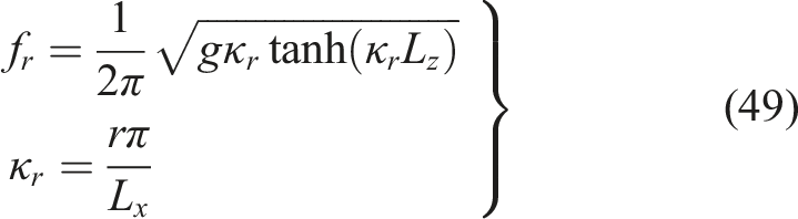
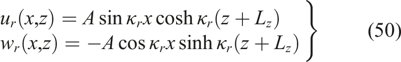
From small-amplitude wave theory, the order-r natural frequency f
r
of the rectangular tank and the order-r natural modes u
r
and w
r
for the horizontal and vertical velocities, respectively, are given by Faltinsen and Timokha (2009)
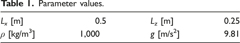
Parameter values.
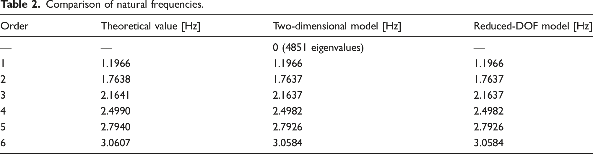
Comparison of natural frequencies.
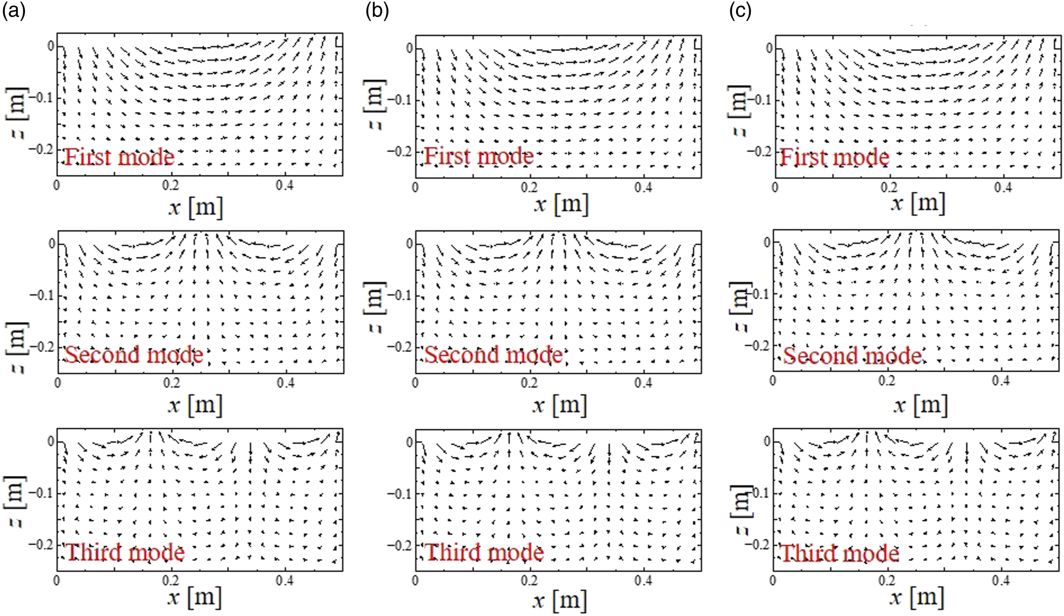
Comparison of shapes of natural modes. (a) Theoretical modes (equation (50)). (b) Two-dimensional model. (c) Reduced-DOF model.
However, zero-frequency natural frequencies appear in the two-dimensional model (Table 2) because the stiffness matrix is singular. There are 4851 zero-frequency eigenvalues, and that number increases with the number of vertical separations. With a zero-frequency natural mode, the water surface does not move. By contrast, the reduced-DOF model has no zero-frequency natural frequencies, and its other natural frequencies agree exactly with those of the two-dimensional model. In addition, the reduced-DOF model reproduces the natural modal shapes of the two-dimensional model (Figure 9(c)). Therefore, our method for reducing the number of DOFs is valid.
This linear problem has the theoretical solution of equation (49) and (50). However, actual sloshing is a nonlinear phenomenon and differs from the theoretical solution when the amplitude is large. We confirm the validity of the nonlinear model in the section Comparison With Experimental Results.
Comparison with experimental results
In this section, numerical results from the nonlinear concentrated mass model are compared with experimental results to assess the validity of the proposed model in the nonlinear region.
Experimental apparatus and analysis method
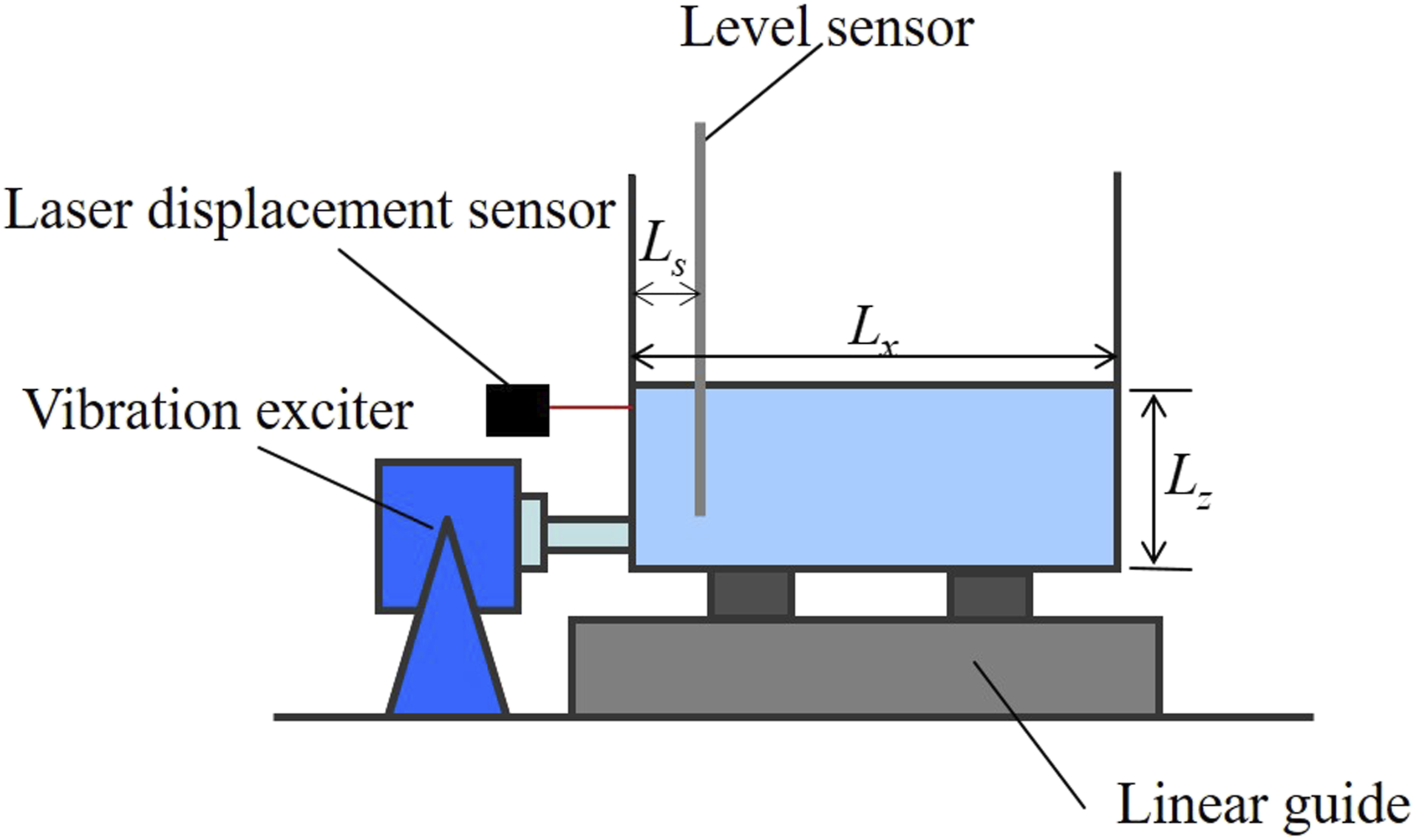
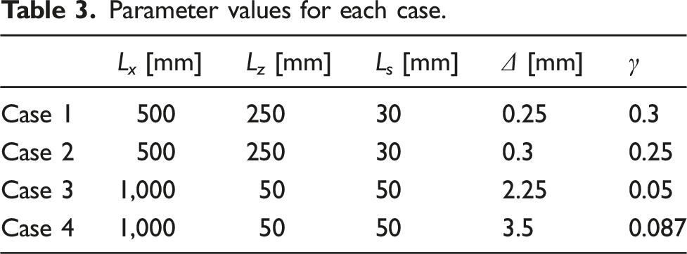
To validate the proposed models, we performed sloshing experiments in a rectangular tank, as shown in Figure 10. The rectangular tank of width 100 mm was formed from 10-mm-thick acrylic boards. It was set on a linear guide and excited horizontally by a vibration exciter. A capacitance-type water-level gauge was installed at a distance of Ls from the left wall. We performed experiments in four configurations, which we refer to as cases 1–4. The values of the horizontal length L
x
, water depth L
z
, and excitation displacement Δ in each case are given in Table 3. In cases 1 and 2, the water was deeper than in cases 3 and 4; the latter two cases satisfy the shallow-water wave condition (i.e., the water depth is less than one-fifth of the wavelength).We assume that the inertial force Experimental apparatus. Parameter values for each case. Frequency responses (reduced-DOF model). (a) Case 1. (b) Case 2. (c) Case 3. (d) Case 4.
Experimental and numerical results
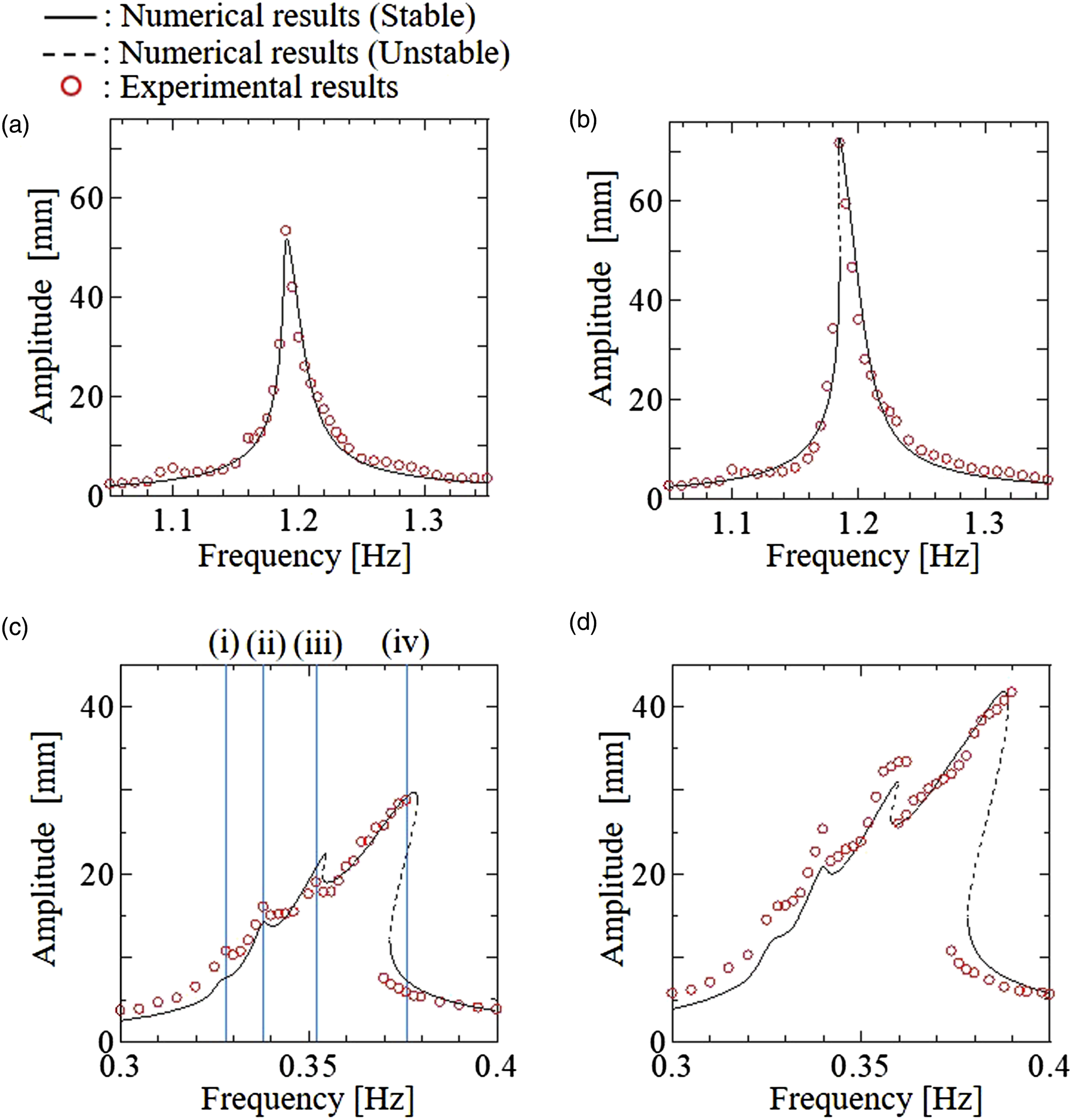
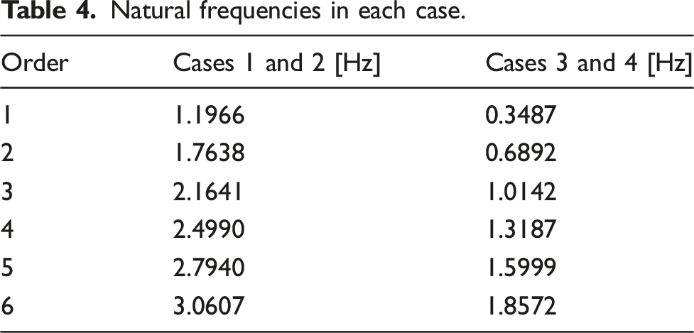
For cases 1 and 2 (deep water), Figure 11(a) and (b) show the frequency responses around the first-order resonance. The linear first-order natural frequency is 1.20 Hz. The resonance curves tilt slightly to the left in these cases. In general, the resonance curve tilts to the left when L z /L x > 0.337 (Flanagan and Timokha, 2009), and in cases 1 and 2 we have L z /L x = 0.5. The numerical results agree well with the experimental results, and the numerical results calculated using the reduced-DOF model agree well with those calculated using the two-dimensional model.
Figures 11(c) and (d) show the frequency responses around the first-order resonance for cases 3 and 4 (shallow water) with the reduced-DOF model. The first-order natural frequency is 0.349 Hz. The resonance curves tilt to the right in the case of shallow water. In general, the resonance curve tilts to the right when L z /L x < 0.337, and in cases 3 and 4 we have L z /L x = 0.05. In cases 3 and 4, there are some peaks around the first-order resonance, and at these peak frequencies, solitary waves move back and forth in the tank (Ishikawa et al., 2016). From Figure 11, the numerical results from the proposed model agree well with the experimental results. Therefore, the proposed model is valid for numerical analysis of nonlinear sloshing phenomena.
Natural frequencies in each case.
Conclusions
We proposed a concentrated mass model for analyzing nonlinear two-dimensional sloshing in a rectangular tank, and our conclusions are as follows. 1. A concentrated mass model was proposed for two-dimensional sloshing in a rectangular tank excited horizontally. The restoring forces were derived from static and dynamic pressures, the latter of which considers vertical acceleration of the z nodal points. 2. A method for reducing the number of DOFs of the proposed two-dimensional model was proposed, by which the number of DOFs in the vertical direction can be reduced to one. 3. The advantage of the proposed method is that DOFs of the model are less than that of the two-dimensional finite-element method, thereby reducing the computation time dramatically. 4. The natural frequencies in a rectangular tank as obtained from the concentrated mass model (two-dimensional and reduced-DOF models) agreed well with the theoretical natural frequencies. 5. The numerical results agreed well with the experimental results both qualitatively and quantitatively. 6. In a tank with complex shape, the water depth varies from location to location. In this case, the water area is divided into rectangular elements, and the DOF reduction is performed at each location to apply the proposed model to the tank with complex shape. In the case of a three-dimensional problem, the water region is divided into rectangular parallel-piped elements, and mass points are located at the faces of the elements. However, these models have not been validated, and doing so is a future task, along with modeling the damping.
Footnotes
Acknowledgments
The authors would like to thank Mr Yuki Amano at the Railway Technical Research Institute and Prof. Kenichiro Matsuzaki at Kagoshima University for discussions about this research. The experimental equipment was made by Mr Yosuke Koba at Kyushu University.
Declaration of conflicting interests
The author(s) declared no potential conflicts of interest with respect to the research, authorship, and/or publication of this article.
Funding
The author(s) received no financial support for the research, authorship, and/or publication of this article.