Model Selection in Continuous Test Norming With GAMLSS

Abstract

To compute norms from reference group test scores, continuous norming is preferred over traditional norming. A suitable continuous norming approach for continuous data is the use of the Box–Cox Power Exponential model, which is found in the generalized additive models for location, scale, and shape. Applying the Box–Cox Power Exponential model for test norming requires model selection, but it is unknown how well this can be done with an automatic selection procedure. In a simulation study, we compared the performance of two stepwise model selection procedures combined with four model-fit criteria (Akaike information criterion, Bayesian information criterion, generalized Akaike information criterion (3), cross-validation), varying data complexity, sampling design, and sample size in a fully crossed design. The new procedure combined with one of the generalized Akaike information criterion was the most efficient model selection procedure (i.e., required the smallest sample size). The advocated model selection procedure is illustrated with norming data of an intelligence test.

When using psychological tests in practice, normed test scores are required to achieve a sensible interpretation. Normed scores are derived from a raw test score distribution of a reference population. In practice, one resorts to collecting test scores among a representative sample of the reference population. Based on these test scores, the raw test score distribution is estimated. When multiple reference populations are involved for the same test, for example, depending on gender or age, and the raw score distributions differ between these populations, different norms should be provided. Traditionally, the distributions, and thus the norms, were estimated for the different subgroups. For each subgroup, norm tables were created that convert the raw scores into normed scores.

The main limitation of traditional norming is that all demographic variables are treated as discrete values, also those that are continuous in nature. This approach is built on the assumption that the score distributions are the same for all continuous values within a subgroup. This assumption may be unrealistic in practice, yielding suboptimal norms. In the Wechsler Intelligence Scale for Children–Third edition (WISC-III-NL; Kort et al., 2002; Wechsler, 1991), a difference in age of 1 day can lead to a difference in IQ of even 12 IQ-points (Tellegen, 2004), when the test taker moves from one age subgroup to the next. Within traditional norming, a solution for this would be to increase the number of subgroups, but this leads to less precise norms as the sample size per subgroup decreases (Oosterhuis, van der Ark, & Sijtsma, 2016).

To overcome this limitation of discrete values, continuous norming was developed (Gorsuch, 1983), which makes it possible to relate the demographic variables to the test scores on a continuous basis. A statistical model is built that describes the distribution of test scores conditional on the relevant characteristics. In this way, the available information from the entire norm group is used in estimating the norms. This makes sense, as, for example, test scores of 5- and 7-year-old children are informative for test scores of 6-year-old children. As a result, continuous norming requires smaller samples than traditional norming (e.g., Bechger, Hemker, & Maris, 2009; Oosterhuis et al., 2016).

This appealing property is widely recognized, witness the fact that most, if not all, modern tests use continuous norming. Examples are the Wechsler Intelligence Scale for Children–Fourth edition (WISC-IV; Wechsler, 2003), Bayley-III (Bayley, 2006), Wechsler Adult Intelligence Scale–Fourth edition (WAIS-IV; Wechsler, 2008), and the Snijders–Oomen Nonverbal Intelligence Test for 6- to 40-year-old individuals (SON-R 6-40; Tellegen & Laros, 2014).

Various continuous norming methods have been proposed. Zachary and Gorsuch (1985) used standard polynomial regression, with age as a predictor. In such a standard polynomial regression, the means may vary with age, while the distribution at any age is assumed to be normal with constant variance. The latter can be highly unrealistic, yielding serious forms of misfit, with associated improper norms (as discussed in e.g., Van Breukelen & Vlaeyen, 2005). An alternative which allows for varying means as well as varying variances, skewness (and possibly kurtosis), is inferential norming (Wechsler, 2008; Zhu & Chen, 2011). This procedure involves two steps. First, one models the raw score means, variances, skewness, and possibly kurtosis, via polynomial regressions, using the relevant predictor(s), like age. Second, one aggregates the estimated values to generate an estimation of the raw score distributions, from which the norms are derived, typically using some smoothing by hand. This procedure was applied to the WAIS-IV test (Wechsler, 2008). The disadvantages of inferential norming are that Step 1 can be suboptimal in view of Step 2, and that one step involves subjective decisions.

An alternative which involves only one step, is the use of the statistically well-founded generalized additive models for location, scale, and shape (GAMLSS; Rigby & Stasinopoulos, 2005). The GAMLSS framework includes many different distributions. Because of this useful flexibility, most recently applied continuous norming methods fall within this GAMLSS framework. An example is the Bayley-III test norming (Bayley, 2006; Cromwell et al., 2014; van Baar, Steenis, Verhoeven, & Hessen, 2014), which involved a polynomial regression using a Box–Cox t distribution (rather than a normal distribution, as in standard regression).

In this article, we focus on the use of the Box–Cox Power Exponential (BCPE) distribution. All instances of GAMLSS allow for differences in location, most of them also allow for differences in spread, and many of them allow for differences in skewness, or skewness and kurtosis. The BCPE distribution allows for differences in location, spread, skewness, and kurtosis. The application of the BCPE model to test norming requires model selection. This implies that one needs to establish the specific predictors to include in the model. It is very convenient if this can be done with an automatic selection procedure. However, the performance of automatic selection procedures in this context is unknown. Hence, in this study, we will compare the performance of two stepwise model selection procedures: One existing procedure and one that we developed ourselves, combined with various criteria, considering the very flexible BCPE distribution.

The remainder of this introduction is organized as follows. First, we will explain the GAMLSS and the BCPE distributions in more detail. Second, we will explain different model selection criteria and the stepwise model selection procedures. Finally, we will describe our specific research questions.

GAMLSS and BCPE

GAMLSS

The GAMLSS framework allows the modelling of any distribution in the exponential family. GAMLSS has been applied not only in psychological test norming (Bayley, 2006; Cromwell et al., 2014; van Baar et al., 2014), but also in related areas, namely growth chart developing (e.g., Borghi et al., 2006; WHO Multicentre Growth Reference Study Group, 2006) and lung function charts (e.g., Cole et al., 2009; Quanjer et al., 2012). Growth charts express references for measures like length as a function of age. In lung function research, spirometry indices (i.e., measuring of lung function) are modelled as a function of age.

BCPE

In this article, we focus on the BCPE distribution (Rigby & Stasinopoulos, 2004). The BCPE is a highly flexible distribution, useful for variables on a continuous scale. The BCPE is able to model any type of kurtosis (lepto, platy, and mesokurtosis), while, for example, the BCT distribution does not allow for a platykurtic distribution. This flexibility is important, as Rigby and Stasinopoulos (2004) showed that both refraining from and incorrect modelling of skewness and kurtosis can lead to distorted fitted percentiles. To estimate the norms properly, it is important that the distributional parameters are estimated properly. The four parameters of the BCPE distribution relate to the location (µ, median), scale (σ, approximate coefficient of variation), skewness (ν, transformation to symmetry), and kurtosis (τ, power exponential parameter). The BCPE distribution simplifies to a normal distribution when ν = 1 and τ = 2 (Rigby & Stasinopoulos, 2004).

Automated Model Selection

The key in using the BCPE for continuous norming is to allow the four parameters of the BCPE distribution to vary with the continuous predictor, for example, age. The relationship between these four parameters and age can take different forms. To capture this, we need a flexible model for each of the four parameters. In this study, we do this with polynomials, for example, µ = β₀ + β₁ age + β₃ age². We make use of orthogonal polynomials to avoid multicollinearity between the various terms in the polynomial. As the number of possible models is infinitely large, it is important to have an automated approach, based on a particular selection criterion that finds optimal choices for µ, σ, ν, and τ.

Selection Criteria

Commonly used model selection criteria are the generalized Akaike information criterion (GAIC; Akaike, 1983; Rigby & Stasinopoulos, 2006) and cross-validation (Geisser, 1975; Stone, 1974). Both the GAIC and cross-validation try to prevent overfitting of the data, which increases the generalizability to other data of the same type (Hawkins, Basak, & Mills, 2003). After all, we do not want to accurately estimate the norms for the reference sample, but for the reference population. This prevention of overfitting is done indirectly by the GAIC, where the number of parameters is penalized, and directly by cross-validation, where the model’s prediction of new, unseen data is evaluated.

The GAIC is given by

$$\mathrm{GAIC}(p)=-2{\widehat{\ell }}_d+p.df,$$

(1)

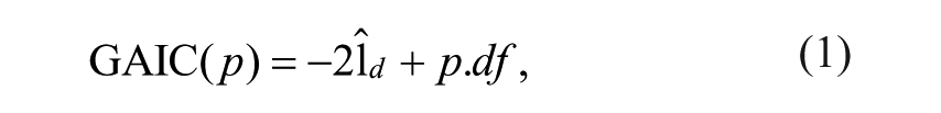
where p indicates the penalty, ${\widehat{\ell }}_d$ the fitted log-likelihood of the data, and df the total effective degrees of freedom used in the model. The value p of the penalty determines the trade-off between the fit and the complexity of the model. The higher the penalty, the higher the penalization of the addition of parameters. In general, the fit increases when the degree of the polynomial is increased (i.e., parameters are added), but this increase in fit has to be in proportion with the resulting increase in complexity.

In our study, we look at three special cases of the GAIC, namely the Akaike information criterion (AIC; Akaike, 1974) where the penalty p = 2, the Bayesian information criterion (BIC; Schwarz, 1978) where the penalty p = ln(n) and n is equal to the sample size, and the GAIC(3) where the penalty p = 3. These three penalties were also used by Rigby and Stasinopoulos (2004, 2006). According to Stasinopoulos and Rigby (2007), the penalty p = 3 appeared to be a reasonable compromise between the AIC and BIC. For each special case of the GAIC, we selected the model with the lowest criterion value.

In K-fold cross-validation, the data are split into K equal parts. For each k = 1, . . . , K, the kth part is removed from the data set, the model is fitted to the remaining K − 1 parts of the data (training set), and then predictions are made for the left-out kth part (validation set). The K parts are C₁, C₂, . . . , C_K, where C_k refers to the observations in part k. The cross-validated global deviance is as follows:

$${\mathrm{CV}}_{(K)}={\displaystyle \sum _{k=1}^K-2{\widehat{\ell }}_k},$$

(2)

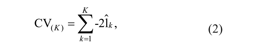
where $\widehat{{\ell }_k}$ is the fitted log-likelihood, based on a model fitted to the K − 1 part of the data and evaluated at the kth part of the data.

There is a bias-variance trade-off associated with the choice of K. When K = n, the cross-validation estimator is approximately unbiased for the true (expected) prediction error. However, it can have a higher variance than for K < n, because the n training sets are very similar to one another (Hastie, Tibshirani, & Friedman, 2009). Multiple studies have found that K = 10 is a good compromise in this bias-variance trade-off (e.g., Breiman & Spector, 1992; Davison & Hinkley, 1997; Kohavi, 1995). We selected the model with the lowest global deviance.

Model Selection Procedures

The GAMLSS R package (Stasinopoulos & Rigby, 2007) includes two stepwise model selection procedures—denoted in the package by “Strategy A” and “‘Strategy B”—that allow for the selection of all distribution parameters. Because these procedures may not be optimal, as motivated below, we developed an alternative stepwise model selection procedure.

As we employ orthogonal polynomials in our study, the model for a distributional parameter can be depicted as follows:

$${\displaystyle \sum _{q_k=0}^{Qk}{\beta }_{qk}}{x}^{qk}$$

(3)

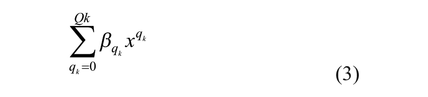
where q_k indicates the degree of the polynomial (q_k = 0, 1, 2, . . . , Q_k) for distributional parameter k ∈ (µ, σ, ν, τ), β indicates the coefficient of the parameter and x indicates the predictor (here: age).

In “Strategy A,” the models for the distributional parameters are selected in a fixed order: first µ, followed by σ, then ν, and finally τ. That is why, we refer to this procedure as the fixed order procedure. To apply this model selection, one needs to select a scope of models, which includes a range of terms for consideration, and an initial model, M⁰, needs to be selected. The initial model should be small, for example, including a linear term for µ (i.e., Q_µ = 1), and only intercepts for σ, ν, and τ (i.e., Q_σ = Q_ν = Q_τ = 0). For short, we denote this model as poly(X, 1, 0, 0, 0).

The selection of the parameters involves successive forward selection procedures for Q_µ, Q_σ, Q_ν, and Q_τ, followed by backward selection procedures for successively Q_ν, Q_σ, and Q_µ to decide whether either the parameters selected in the forward selection (i.e., Q_k) or an intercept (i.e., Q_k = 0) should be included in the final model, given the chosen models for the other distributional parameters. This fixed order is in line with the idea of the authors of the GAMLSS R package that the parameter hierarchy (i.e., sequentially µ, σ, ν, τ) has to be respected (help function of GAMLSS R package version 5.0-1; Rigby & Stasinopoulos, 2005). The model selection of the fixed order procedure is based on one of the special cases of the GAIC.

“Strategy B” uses the same procedure as the fixed order procedure, but each term in the scope is fitted to all four distributional parameters, rather than one distributional parameter at a time. As a result, the value of Q_k is the same for all four distributional parameters k. We will not evaluate this procedure because we believe it too restricted; we see no reason to assume, for instance, that the polynomial degree of the relationship between age and the median score equals that between age and the kurtosis of the scores.

We believe that the fixed order procedure is not optimal and we provide two arguments for this. First, in the fixed order procedure, the distribution parameters are modelled in a hierarchical order (first µ, then σ, followed by ν, and finally τ). We believe that it is logical to, for example, extend the model for τ before that of µ when this results in a better model fit.

Second, in the backward elimination part of the fixed order procedure, it is only checked whether the parameters that are found in the forward selection for that particular distributional parameter are needed. So, if a fourth degree polynomial of age is found for µ, it is only checked whether it is better to keep this parameter or to use an intercept. However, we believe it would be better if other polynomial degrees are considered as well. That is why, we developed a new stepwise selection procedure, which we term the free order procedure, that deals with these issues.

In the free order procedure, the models for the distributional parameters are selected in a relatively free order. The free order procedure always starts with model M⁰ = poly(X, 1, 0, 0, 0). Subsequently, four forward models are fitted, denoted as M1Fµ $M_{F_{\mu }}^1$ , $M_{F_{\sigma }}^1$ , $M_{F_{\nu }}^1$ , and $M_{F_{\tau }}^1$ . In each of these models, for distributional parameter k corresponding to model ${\mathrm{M}}_{F_k}$ , Q_k is increased by one. In addition, if Q_k > 0, a backward model is fitted for distributional parameter k. In the first step of this procedure, only a backward model for µ can be fitted, which is the intercept only model, M¹ _{B µ} $M_{F_{\mu }}^1$ = poly(X, 0, 0, 0, 0).

The value of the specific model selection criterion is calculated for all fitted models (i.e., the initial model, the four forward models, and the backward model). The model with the best (i.e., lowest) criterion value is selected, which then becomes ${\mathrm{M}}^{\mathrm{s}}$ . Then, the criterion value of model ${\mathrm{M}}^{\mathrm{s}}$ is compared with those of the four forward models, M^s+1 _{F µ}, M^s+1 _{F σ}, M^s+1 _{F ν} $M_{F_{\nu }}^{s+1}$ , and M^s+1 _{F τ}, and the, at most four, backward models, M^s+1 _{B µ}, M^s+1 _{B σ}, M^s+1 _{B ν}, and M^s+1 _{B τ}. This process is repeated until model $M^s$ has the best value of the chosen criterion.

The advantage of the free order procedure over the fixed order procedure is that the model selection is flexible: the order of the distributional parameters which are updated is not fixed beforehand, but depends on the model fit, and the backward selection allows going back one degree of the polynomial instead of choosing between a certain degree and the intercept.

Research Questions

The goal of this study is to compare the performance in estimating norms in the context of developmental and intelligence tests, using two stepwise model selection procedures (fixed order and free order) and four model selection criteria, AIC, BIC, GAIC(3), and cross-validation. The performance is assessed considering the difference in the population and model-implied distributions of scores. In our study, we systematically varied the population model, sample size, and sampling design. We included nine different population models, varying in complexity of the relationship between age and the different distributional parameters. The sample size N was equal to 100, 500, or 1,000. The sampling design was uniform or weighted. In uniform sampling, we simulated age values equally spread across the age range. In weighted sampling, the number of people included with a certain age value depended on the change in median test score around that age value: the larger the change in test score, the more people with that age value included. We applied uniform sampling across all population models, while we applied weighted sampling only to the simplest population model. For each condition, we generated 500 data sets. As a result, 500 (replication) × 9 (population model) × 3 (sample size) = 13,500 different data sets were obtained to which uniform sampling was applied. On the other hand, 500 (replication) × 1 (population model) × 3 (sample size) = 1,500 different data sets were obtained to which weighted sampling was applied. Hence, the total number of different obtained data sets was 15,000. To each data set, we applied the two different stepwise model selection procedures (i.e., fixed order and free order procedure), combined with three GAIC model selection criteria (AIC, GAIC(3), BIC) and cross-validation.

Regarding the population model, we expected the simpler data conditions to outperform the more complex data conditions. Regarding the sampling design, we expected the weighted sampling to outperform the uniform sampling in the simplest data condition, because more information is expected to be available when more changes in distributions are to be estimated.

Regarding the sample size, we expected conditions with larger sample sizes to outperform those with smaller sample sizes, because with increasing sample size the probability that the sample represents the population increases, and thus, the precision of estimate would be higher. In addition, we expected this effect to be more pronounced for the weighted sample conditions than the uniform sample conditions, as the number of observations is extremely small for some age ranges with weighted sampling (i.e., interaction sample size and sampling design).

Regarding the two stepwise model selection procedures, we expected that the free order procedure yields a better fitting model than the fixed order procedure because the free order procedure is more flexible. We did not have clear expectations for the model selection criteria.

The root mean squared error can be split up in a bias and a variance component. We will briefly look at the effect of all conditions on bias and variance separately.

Method

Data Generation

To generate the simulated data, we used the BCPE distribution within the GAMLSS framework. The four distributional parameters are modelled using monotonic link functions. We have used the default link functions for the BCPE distribution, namely an identity link for µ and ν, and a log link for σ and τ (Stasinopoulos & Rigby, 2007). The log link makes sure that the values for the distributional parameters stay positive. Even though µ has to be positive, we have chosen to use the identity link for µ as this leads to additive effects on µ, which makes the interpretation easier. As it turns out, all estimates for µ are positive with this identity link function as well, further reducing the need for a log link function.

The penalized log likelihood function can be maximized iteratively using the Rigby and Stasinopoulos (1996), the Cole and Green (1992) algorithm, or a combination of both algorithms (see Appendix B of Rigby & Stasinopoulos, 2005, for a detailed explanation of both algorithms). We have chosen to use the Rigby and Stasinopoulos algorithm only because it is more stable than the Cole and Green algorithm. To make sure that, on the one hand, the number of iterations was enough to reach convergence, but, on the other hand, the study remained feasible, we have set the maximum number of iterations equal to 10,000.

Population Models

The population models differ in the relationship between age and the distributional parameters (i.e., µ, σ, ν, or τ). The models were chosen such that they differ in complexity of the distributions, and such that they are realistic representations of models relevant in the context of developmental and intelligence tests.

In all conditions, the median score µ depends on age. The reason for this is that we believe it is unrealistic to assume that this relationship does not exist in developmental and intelligence tests. Hence, we only varied the dependency of the other three distributional parameters on age. The population models result from a completely crossed 2 × 2 × 2 design, with σage (dependent, independent) × νage (dependent, independent) × τage (dependent, independent), plus a ninth model, with all parameters (µ, σ, ν, and τ) age dependent and µage more complex. We named the nine resulting population models “1000,” “1100,” 1010,” “1001,” “1110,” “1101” “1011,” “1111,” and “complex,” where the “1” refers to age dependence and “0” refers to age independence of the distributional parameters “µσντ.” In addition, “complex” refers to the ninth model, in which there is age dependence for all distributional parameters and the age dependence for µ is more complex than in the other models.

The age dependence of the distributional parameters is expressed in Table 1 and visualized in Figure 1 for the various conditions. We have chosen these relationships because those relations resemble those found in the norming data of the intelligence test SON-R 6-40 (Tellegen & Laros, 2014). We made the values of ν range from −2 (age = 5) to 4 (age = 40), and the values of τ from 1 (age = 5) to about 3 (age = 40). Recall that the BCPE distribution simplifies to a normal distribution when ν = 1 and τ = 2 (Rigby & Stasinopoulos, 2004). Hence, the distribution ranges from a positively skewed (ν < 1) to negatively skewed (ν > 1), expressing floor and ceiling effects, respectively. In addition, the distribution ranges from leptokurtic (τ < 2) to platykurtic (τ > 2).

Table 1.

Relationship Between Age and the Distributional Parameters in the Simple and Complex Data Conditions.

Parameter	Age dependence	Age independence
µ (Simple)	$220{\left({\left(age+2\right)}^{1.4}\right)}^{-1}+20$	—
µ (Complex)	$\frac{60}{13}{\left(575\left(age+2\right)-2\sin \left(\frac{age}{2}\right)\right)}^{-1}+\frac{12}{13}$	—
σ	$\exp \left(-0.0029{\left(age-23.5\right)}^2-1.4\right)+0.0001$	0.17
ν	$\frac{1}{35}\left(6\mathrm{age}-100\right)$	1
τ	$\exp \left(0.0314\mathrm{age}+0.1886-0.3781\right)$	2

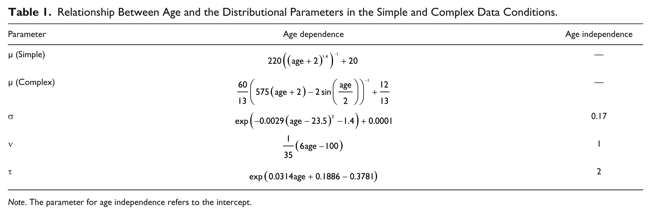
Note. The parameter for age independence refers to the intercept.

Figure 1.

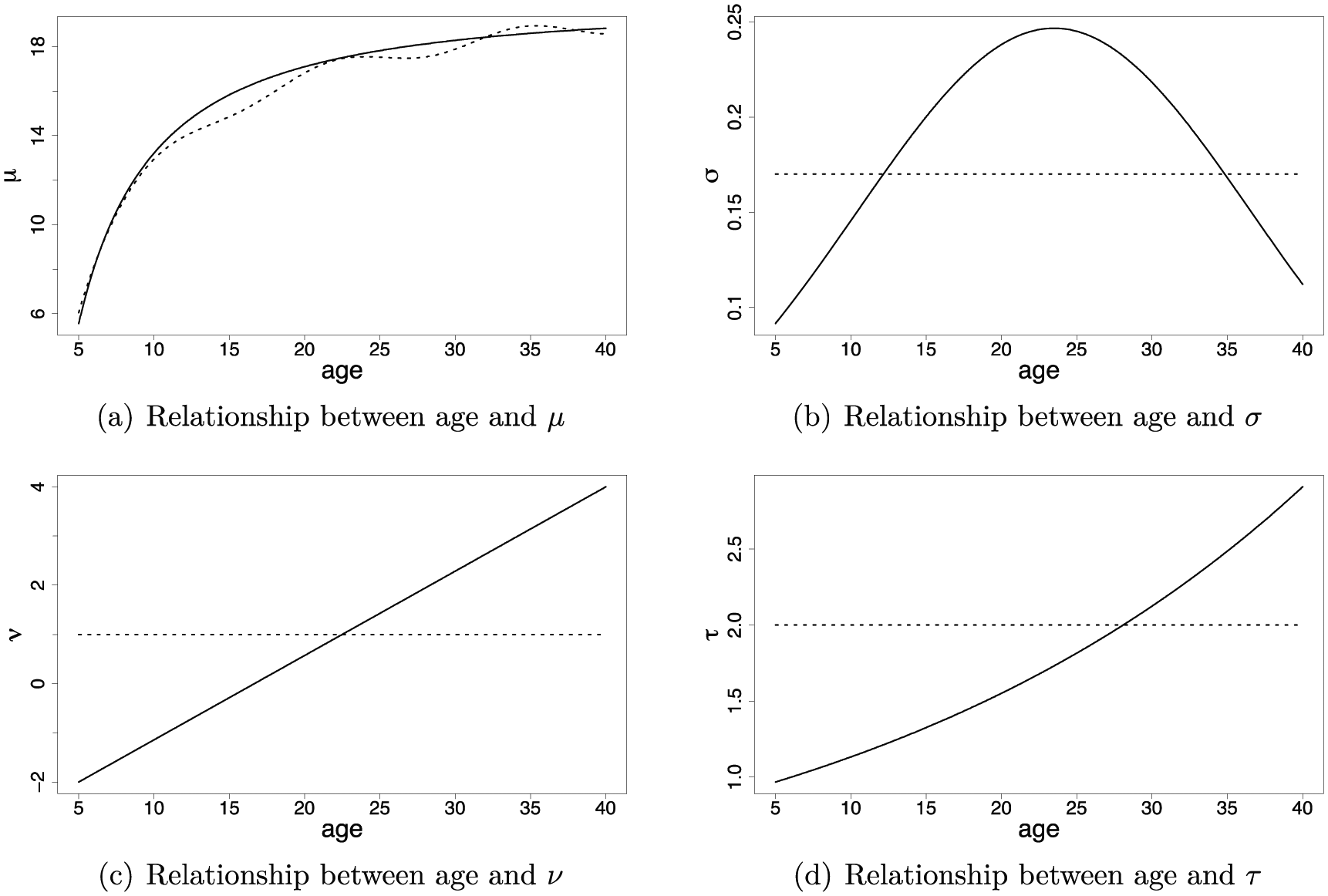
The relationships between age and each of the distributional parameters.

Examples of the resulting probability density functions (PDFs) for the ages 8, 22, and 35 in the population are presented in Figure 2. Panel (a) shows the PDFs for the simplest population model, “1000,” and panel (b) shows the PDFs for population model “1111.” The first model shows how age dependency for µ only looks like, and the latter model shows what the age dependency for all four distributional parameters looks like (except for the more complex relationship for µ in model “complex”).

Figure 2.

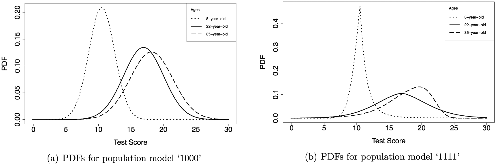
The probability density functions (PDFs) for population model “1000”, with age dependence for µ only, panel (a), and “1111”, with age dependence for µ, σ, ν, and τ, panel (b).

Sampling Design

We have two different sampling designs of age values: uniform sampling and weighted sampling. In uniform sampling, we generated N age values uniformly distributed from 5 to 40, which is the age interval relevant for the SON-R 6-40. In weighted sampling, we included more (simulated) people of a certain age when we expected more change in the median test score for that age. More specifically, we generated a weighted sample of age values based on the first derivative of the formula of µ, which is dependent on age. As we expected the positive effect of weighted sampling to be most pronounced in the simplest data condition, where only µ depends on age, we only applied weighted sampling to this simplest data condition.

The function of µ becomes almost flat for age values above 25. Hence, to avoid that the sample almost only consists of age values below 25, the sample weights consisted not only of the first derivative of the formula of µ, but we also added a constant. This constant was set equal to the mean of the values of the first derivatives. As population of age values, we generated N values uniformly distributed from 5 to 40. Using the weights explained above, we sampled (with replacement) N values from this population of age values. In the models with the more simple relationship between µ and age (Models 1 to 8), the median and mean of the age values are 14.02 and 17.18, respectively. In the models with the more complex condition between µ and age (Model 9), the median and mean of the age values are 13.27 and 16.72, respectively. The thus sampled age values were used across all replications.

Test Score Simulation

The test scores resulting from the distribution parameters (i.e., µ, σ, ν, and τ) are randomly drawn from the Box–Cox power exponential distribution with the specific distributional parameters belonging to a specific age value.

Examples of percentiles (i.e., 5, 15, 25, 50, 75, 85, 95) as a function of age under the simplest and most complex population models with randomly drawn observations with uniform sampling (N = 500) are visualized in Figure 3.

Figure 3.

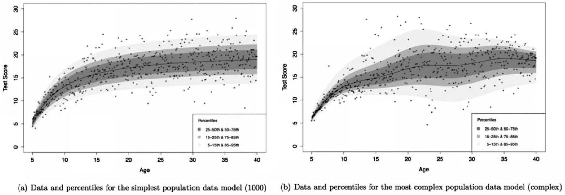
The percentiles under the population model with uniform sampling and N = 500, and the randomly drawn observations under this model for one replication (black dots).

Model Selection

We used the program R (R Core Team, 2015) for model estimation. The model parameters and distributions were estimated with the GAMLSS R package (version 5.0-1; Rigby & Stasinopoulos, 2005), which was also used for constructing the estimates using the fixed order procedure. The R code for the free order procedure is available as supplementary material. The cross-validation was performed using the GAMLSS R package. As cross-validation was not implemented in the fixed order procedure, we wrote R code for this ourselves.

A scope of fitted models had to be specified for both procedures. In the fixed order procedure, we used as the scope of fitted GAMLSS models for µ, ln(σ), ν, and ln(τ), the intercept as lower bound and a polynomial fit of degree 7 as upper bound. This upper bound was chosen because parameters from polynomials of degree 8 onward were in general too complex to be estimated, as indicated by nonconvergence. In creating the fixed order procedure in combination with cross-validation, we even had to set the upper bound for τ to a polynomial fit of degree 2 because there was (almost) no convergence possible with higher degree polynomials.

In the free order procedure, we used as the scope of GAMLSS models for µ, ln(σ),ν, and ln(τ), the intercept as lower bound and a polynomial of degree 20 as upper bound. The scope of models is larger for the free order procedure than for the fixed order procedure. The reason for this is that for the fixed order procedure, this upper bound of models is always fitted for each of the distributional parameters, while this is not necessarily the case for the free order procedure. In the free order procedure, we start with a simple model and a polynomial of a particular degree is only fitted if the previous degree fitted well. So, models with very high-degree polynomials, like degree 20, are extremely unlikely to be fitted. We did only include this parameter in the scope to make sure that the scope was large enough.

Note that the model to generate the data differs from the fitted models. So, we did not generate the population models with orthogonal polynomials. This was done to examine the stability over these kind of differences, as in empirical practice the fitted model will not comply with the data-generating model, if such a generating model would exist at all.

Outcome Variable

As the outcome variable, we consider the difference between the PDFs conditional on age in the population, and the probability density distributions conditional on age implied by the estimated model. The difference between the population and model-implied distributions is as follows:

$$f_{XY}(xy)-{\widehat{f}}_{XY}(xy),$$

(4)

where f_XY is the PDF for test scores Y and age X. This difference is expressed as one value D when marginalizing out age x and test score y with

$$D=\sqrt{{\int }_{xy}{(f_{XY}(xy)-{\widehat{f}}_{XY}(xy))}^{2}dydx.}$$

(5)

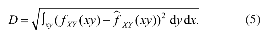
Thus, D is equal to the root mean squared error, and the integral has been numerically approximated in R using standard numerical integration techniques.

Our outcome measure D captures both variance and bias, as D² = Var + Bias², where Bias is defined as follows:

$$\mathrm{Bias}={\int }_{xy}(f_{XY}(xy)-{\widehat{f}}_{XY}(xy))dydx,$$

(6)

and Var is defined as follows

$$\mathrm{Bias}={\int }_{xy}(f_{XY}(xy)-{\widehat{f}}_{XY}(xy))dydx,$$

(7)

In words, the bias tells us how much the expected value of an estimator deviates from its population value. Variance tells us how large the deviations are between the estimates and the expected value of the estimator.

Results

Effect Sizes

Tables 2, 3, and 4 show the median and SD for the value of D in each condition, for sample sizes N = 100, 500, and 1,000, respectively.

Table 2.

Median (SD) Deviances Between the Population and Model-Implied Distributions (D) for N = 100, for Combinations of Model Selection Procedure, Model Selection Criterion, and Data Condition.

Sampling	Weighted	Uniform
Model	1000	1000	1100	1010	1001	1110	1101	1011	1111	Complex
AIC
Fixed	5.080 (11.823)	4.960 (7.771)	5.694 (21.966)	5.114 (6.263)	5.706 (8.412)	5.968 (12.556)	6.277 (78.141)	6.129 (66.984)	6.703 (14.382)	6.838 (11.740)
Free	1.723 (2.532)	1.589 (0.981)	1.927 (1.581)	1.856 (1.484)	2.206 (3.469)	2.282 (1.634)	2.752 (2.621)	2.249 (3.109)	2.805 (3.654)	2.961 (2.698)
BIC
Fixed	4.470 (31.659)	4.059 (44.327)	5.418 (18.75)	4.657 (9.369)	5.118 (14.953)	5.610 (38.318)	6.228 (34.595)	6.192 (23.324)	7.115 (19.615	7.068 (17.565)
Free	1.751 (1.435)	1.539 (0.828)	1.953 (1.539)	1.938 (1.226)	2.269 (1.542)	2.390 (2.125)	2.868 (2.049	2.274 (2.460)	2.943 (3.013)	3.033 (2.320)
GAIC(3)
Fixed	5.045 (23.023)	4.870 (9.137)	5.773 (17.294)	4.879 (16.025)	5.621 (12.664)	5.785 (25.804)	6.478 (14.845)	6.228 (67.693)	7.060 (15.252)	6.963 (19.257)
Free	1.612 (1.72)	1.570 (0.773)	1.973 (1.813)	1.918 (1.427)	2.242 (2.437)	2.311 (1.560)	2.800 (2.486)	2.249 (2.534)	2.826 (3.052)	3.006 (2.374)
CV
Fixed	1.926 (0.515)	1.925 (0.560)	2.307 (0.661)	2.300 (0.620)	2.495 (0.561)	2.521 (1.005)	2.865 (0.631)	2.514 (0.727)	2.896 (0.910)	2.985 (3.827)
Free	2.057 (0.571)	1.996 (0.625)	2.490 (0.645)	2.560 (0.514)	2.559 (0.527)	2.852 (0.585)	3.089 (0.573)	2.754 (0.630)	3.441 (0.978)	3.200 (0.636)

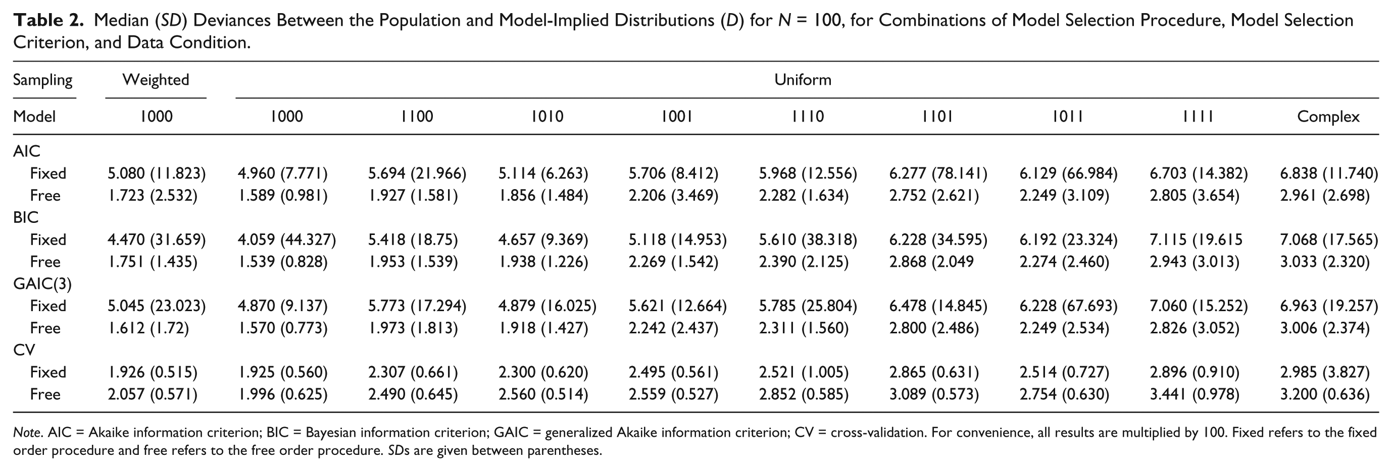
Note. AIC = Akaike information criterion; BIC = Bayesian information criterion; GAIC = generalized Akaike information criterion; CV = cross-validation. For convenience, all results are multiplied by 100. Fixed refers to the fixed order procedure and free refers to the free order procedure. SDs are given between parentheses.

Table 3.

Median (SD) Deviances Between the Population and Model-Implied Distributions (D) for N = 500, for Combinations of Model Selection Procedure, Model Selection Criterion, and Data Condition.

Sampling	Weighted	Uniform
Model	1000	1000	1100	1010	1001	1110	1101	1011	1111	Complex
AIC
Fixed	0.996 (4.124)	0.878 (2.289)	1.199 (2.902)	1.060 (2.854)	1.082 (6.227)	1.221 (2.927)	1.555 (17.976)	1.315 (2.696)	1.610 (3.173)	1.678 (16.091)
Free	0.758 (0.245)	0.715 (0.186)	0.990 (0.412)	0.782 (0.239)	1.229 (0.625)	0.946 (0.334)	1.464 (0.937)	1.048 (0.328)	1.318 (0.746)	1.350 (0.807)
BIC
Fixed	0.743 (0.254)	0.692 (0.189)	1.089 (0.411)	0.784 (0.314)	1.001 (0.315)	1.027 (0.842)	1.421 (0.489)	1.18 (0.524)	1.551 (1.269)	1.476 (15.443)
Free	0.749 (0.227)	0.693 (0.191)	1.075 (0.279)	0.745 (0.223)	1.732 (0.467)	1.014 (0.326)	1.861 (0.753)	1.148 (0.288)	1.507 (0.556)	1.450 (0.514)
GAIC(3)
Fixed	0.790 (3.376)	0.749 (1.638)	1.086 (2.338)	0.825 (2.055)	0.962 (1.726)	1.018 (2.632)	1.351 (1.635)	1.159 (1.612)	1.472 (2.311)	1.437 (15.645)
Free	0.742 (0.224)	0.685 (0.184)	0.994 (0.350)	0.763 (0.228)	1.613 (0.567)	0.952 (0.313)	1.594 (0.900)	1.052 (0.326)	1.356 (0.649)	1.363 (0.709)
CV
Fixed	0.770 (0.242)	0.685 (0.191)	1.092 (0.296)	0.840 (0.342)	0.994 (0.327)	1.286 (0.385)	1.543 (0.509)	1.335 (0.405)	1.821 (0.700)	1.789 (0.715)
Free	0.754 (0.236)	0.685 (0.213)	1.117 (0.339)	0.996 (0.346)	1.753 (0.177)	1.486 (0.494)	2.262 (0.393)	1.489 (0.344)	2.288 (0.599)	2.311 (0.614)

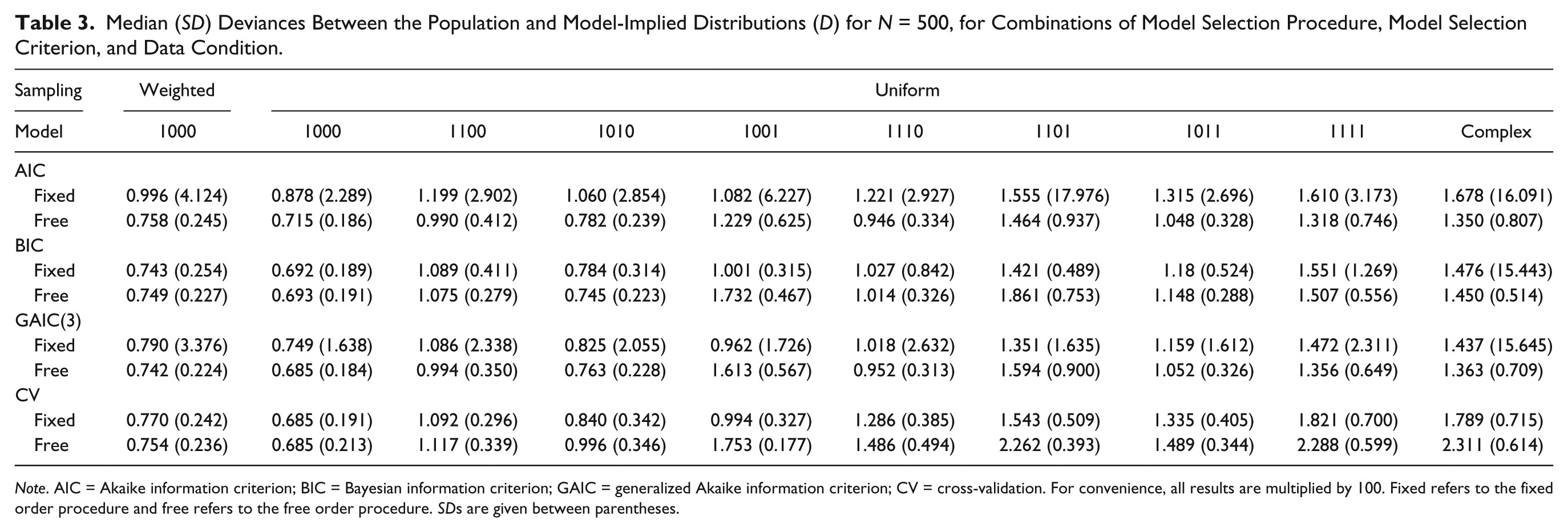
Note. AIC = Akaike information criterion; BIC = Bayesian information criterion; GAIC = generalized Akaike information criterion; CV = cross-validation. For convenience, all results are multiplied by 100. Fixed refers to the fixed order procedure and free refers to the free order procedure. SDs are given between parentheses.

Table 4.

Median (SD) Deviances Between the Population and Model-Implied Distributions (D) for N = 1,000, for Combinations of Model Selection Procedure, Model Selection Criterion, and Data Condition.

Sampling	Weighted	Uniform
Model	1000	1000	1100	1010	1001	1110	1101	1011	1111	Complex
AIC
Fixed	0.585 (0.446)	0.575 (0.238)	0.777 (0.412)	0.633 (0.545)	0.705 (0.297)	0.771 (0.572)	0.966 (0.567)	0.857 (0.499)	1.053 (0.574)	1.043 (0.895)
Free	0.521 (0.141)	0.506 (0.126)	0.704 (0.208)	0.564 (0.137)	0.766 (0.478)	0.647 (0.168)	0.990 (0.497)	0.727 (0.221)	0.904 (0.281)	0.928 (0.298)
BIC
Fixed	0.541 (0.123)	0.529 (0.118)	0.788 (0.193)	0.591 (0.583)	0.732 (0.229)	0.785 (0.224)	1.079 (0.291)	0.878 (0.394)	1.132 (0.305)	1.010 (0.503)
Free	0.542 (0.130)	0.531 (0.122)	0.768 (0.201)	0.581 (0.126)	1.660 (0.435)	0.731 (0.196)	1.461 (0.525)	0.791 (0.205)	1.034 (0.286)	1.033 (0.255)
GAIC(3)
Fixed	0.533 (0.241)	0.522 (0.147)	0.728 (0.362)	0.575 (0.566)	0.656 (0.222)	0.725 (0.495)	0.938 (0.384)	0.799 (0.402)	0.973 (0.458)	0.956 (0.816)
Free	0.515 (0.126)	0.506 (0.124)	0.702 (0.202)	0.562 (0.133)	0.876 (0.498)	0.660 (0.166)	1.059 (0.515)	0.739 (0.198)	0.903 (0.274)	0.946 (0.269)
CV
Fixed	0.561 (0.149)	0.520 (0.135)	0.789 (0.232)	0.597 (0.298)	0.758 (0.295)	0.846 (0.338)	1.171 (0.420)	1.088 (0.380)	1.492 (0.545)	1.409 (0.599)
Free	0.534 (0.140)	0.527 (0.145)	0.796 (0.249)	0.645 (0.268)	1.705 (0.113)	1.322 (0.498)	2.186 (0.396)	1.226 (0.398)	1.911 (0.580)	1.966 (0.647)

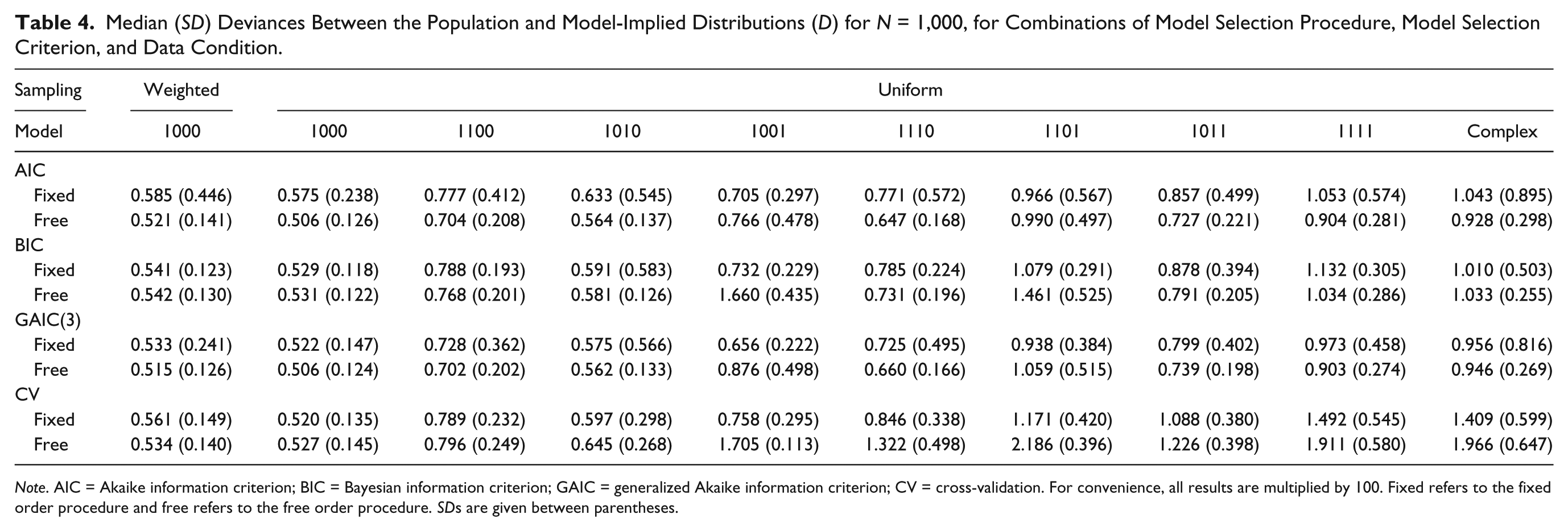
Note. AIC = Akaike information criterion; BIC = Bayesian information criterion; GAIC = generalized Akaike information criterion; CV = cross-validation. For convenience, all results are multiplied by 100. Fixed refers to the fixed order procedure and free refers to the free order procedure. SDs are given between parentheses.

To obtain insight into the effects of the factors on our outcome measure D, a full-factorial mixed effects analysis of variance (ANOVA) was performed. Because the procedure (fixed order, free order) and selection criterion, AIC, BIC, GAIC(3), were run on a single simulated data set, these two factors are within factors. Sample size (N = 100, 500, or 1,000), sampling design (weighted, uniform), and data condition are between factors. Note that we applied weighted sampling to the simplest data condition (“1000”) only, which made a full-factorial design impossible. That is why we performed two full-factorial subanalyses: one analysis with only uniform sampling and one analysis with only the simplest data condition (“1000”). The latter analysis made it possible to compare weighted sampling with uniform sampling.

The total number of observations, resulting from 500 replications for each of the conditions, excluding weighted sampling, would have been 108,000. However, because of missingness due to nonconvergence of the algorithm, the resulting number of observations for this mixed ANOVA was 91,147. The conditions with most missing observations were those with N = 100 (36.5% vs. 5.5% for N = 500, and 4.8% for N = 1,000), the free order procedure (22.7% vs. 8.5% in the fixed order procedure), and the more complex data conditions. The missingness was 26.9%, 19.8%, and 18.3% in the “1011,” “1111,” and complex data conditions, respectively, while it was 8.5% in the simplest data condition (i.e., “1000”). This difference makes sense, as more difficult data need to be modelled with less data. In addition, unlike the free order procedure, the selection is carried out until the end in the GAMLSS fixed order procedure function, even in the presence of nonconvergence of a model (Stasinopoulos, Rigby, Voudouris, Heller, & De Bastiani, 2015). The total number of observations in the mixed ANOVA with only the simplest data condition should have 24,000 observations, but did have 21,916 observations.

With the large number of replications for each condition, it is likely that the mixed effects ANOVA has large power to detect even small differences. That is why, we focused on effect sizes (partial η²) rather than significance tests. Tables 5 and 6 show the values of partial η², the F values, and the corresponding degrees of freedom from the two mixed effects ANOVAs. We consider effects with partial η² < .02 to be too weak to study the corresponding factors in detail. The results from both tables are consistent: There appears to be no effect of data condition and sampling design, and there appears to be a three-way interaction between procedure, selection criterion, and sample size. We do note that the distributions of D values within each cell of the ANOVA design is considerably skewed, and that the variations between conditions differ, thus violating the assumptions of the ANOVA. As ANOVA methods are robust against violations of assumptions (cf. Schmider, Ziegler, Danay, Beyer, & Bühner, 2010) and we only use the ANOVA to flag the “interesting” conditions, we believe these violations are not problematic.

Table 5.

Values of Partial η² From Full-Factorial Mixed Effects ANOVA on D (Leaving Weighted Sampling Out).

Source	Partial η2	F a	df1	df2
Procedure	.079	690.846	1	8,021
Criterion	.128	358.319	3	8,019
Data	.017	17.748	8	8,021
N	.220	1128.701	2	2,207
Procedure × Criterion	.821	581.449	3	8,019
Procedure × Data	.009	9.408	8	8,021
Procedure × N	.082	358.318	2	8,021
Criterion × Data	.005	5.200	24	23,258
Criterion × N	.105	312.726	6	16,038
Data × N	.008	4.014	16	8,021
Procedure × Criterion × Data	.005	5.365	24	23,258
Procedure × Criterion × N	.075	217.114	6	16,038
Procedure × Data × N	.009	4.341	16	8,021
Criterion × Data × N	.009	4.691	48	23,851
Procedure × Criterion × Data × N	.007	3.471	48	23,851

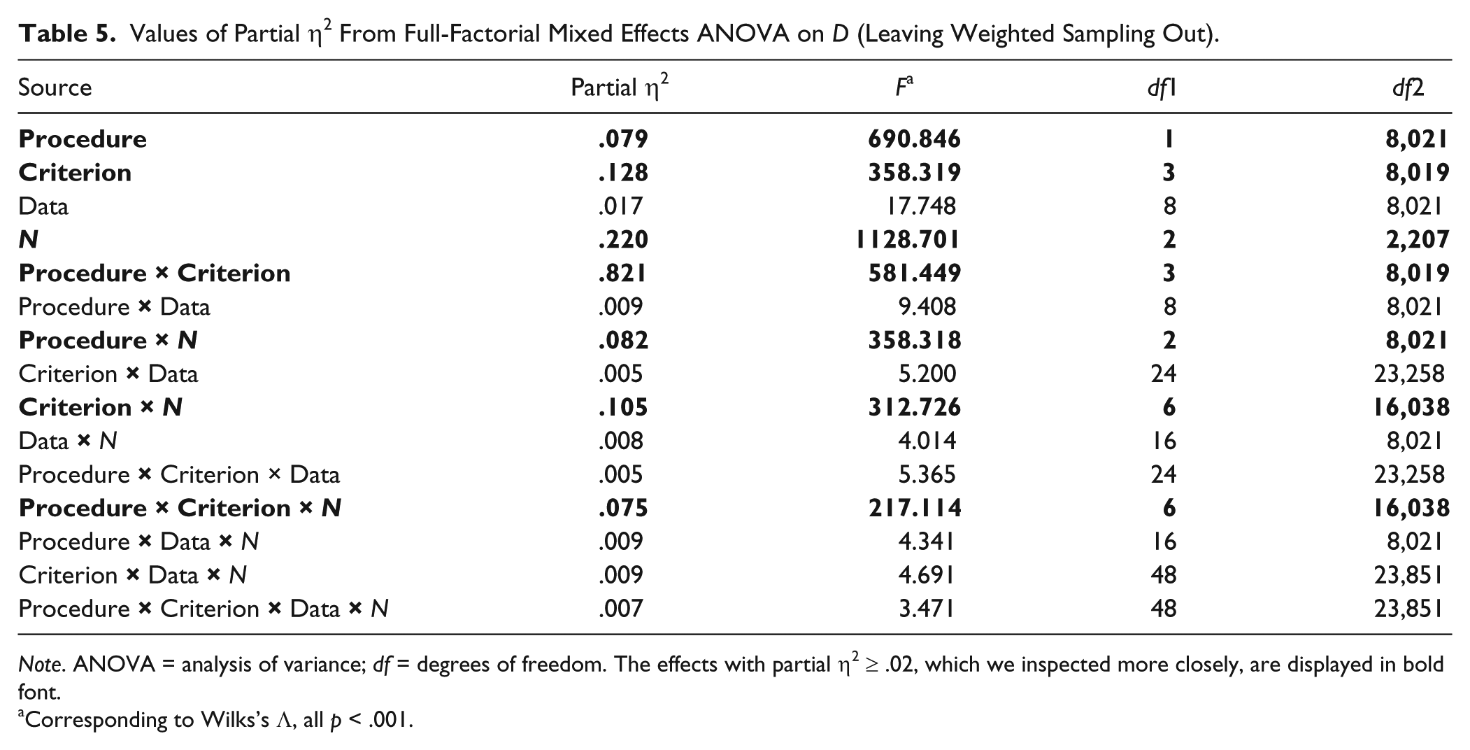
Note. ANOVA = analysis of variance; df = degrees of freedom. The effects with partial η² ≥ .02, which we inspected more closely, are displayed in bold font.

a

Corresponding to Wilks’s Λ, all p < .001.

Table 6.

Values of Partial η² From Full-Factorial Mixed Effects ANOVA on D (For Data Condition “1000”).

Source	Partial η2	F a	df1	df2
Procedure	.085	197.968	1	2,120
Criterion	.207	184.149	3	2,118
Sampling	.008	17.149	1	2,120
N	.153	191.068	2	2,120
Procedure × Criterion	.250	235.167	3	2,118
Procedure × Sampling	.008	16.347	1	2,120
Procedure × N	.083	95.516	2	2,120
Criterion × Sampling	.014	9.916	3	2,118
Criterion × N	.106	83.559	6	4,236
Sampling × N	.013	13.519	2	2,120
Procedure × Criterion × Sampling	.013	9.649	3	2,118
Procedure × Criterion × N	.127	103.062	6	4,236
Procedure × Sampling × N	.011	11.404	2	2,120
Criterion × Sampling × N	.011	8.048	6	4,236
Procedure × Criterion × Sampling × N	.011	7.863	6	4,236

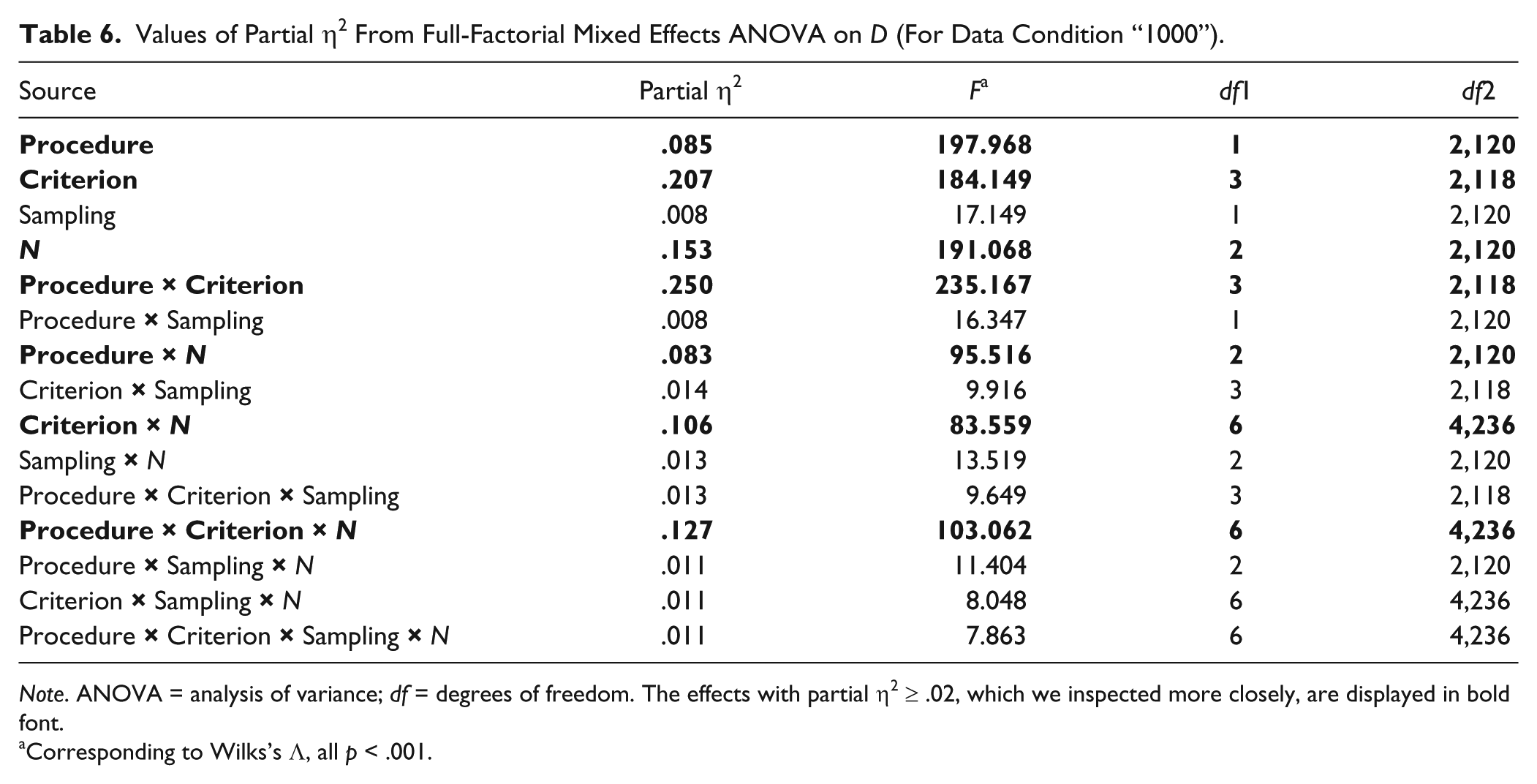
Note. ANOVA = analysis of variance; df = degrees of freedom. The effects with partial η² ≥ .02, which we inspected more closely, are displayed in bold font.

a

Corresponding to Wilks’s Λ, all p < .001.

Interaction Procedure, Selection Criterion, and Sample Size

The main effects, and two-way and three-way interactions between procedure, selection criterion, and sample size are summarized in Figure 4, which shows violin plots with boxplots of the distribution of D for the eight combinations of procedure and selection criterion, for N = 100 (panel a), N = 500 (panel b), and N = 1,000 (panel c). As data condition and sampling design have relatively minor effects (η² < .02), we show the results of one condition, that is, uniform sampling and the simplest data condition. It can be seen that regardless of the procedure and selection criterion used, the value of D becomes smaller as N increases. Moreover, the differences between the different combinations of procedure and selection criterion become smaller as N increases. For N = 100, see Figure 4(a), the free order procedure in combination with one of the GAIC performs better (i.e., has a lower median D value and smaller variance) than the fixed order procedure in combination with one of the GAIC. Cross-validation performs about equal for both procedures. Although the variance in D is smaller for cross-validation compared with the GAIC, the median D values are smaller for the GAIC in combination with the free order procedure than for cross-validation. For N = 500, see Figure 4(b), the performance is about equal for all combinations of procedures and selection criteria, except that the median and variance of D are larger for the fixed order procedure in combination with the AIC, and perhaps the GAIC(3), compared with the other combinations of procedure and selection criterion. For N = 1,000, see Figure 4(c), there seem to be no differences in D between the different combinations of procedure and selection criterion. Again, the fixed order procedure in combination with the AIC performs slightly worse compared with the other conditions, but this difference is very small.

Figure 4.

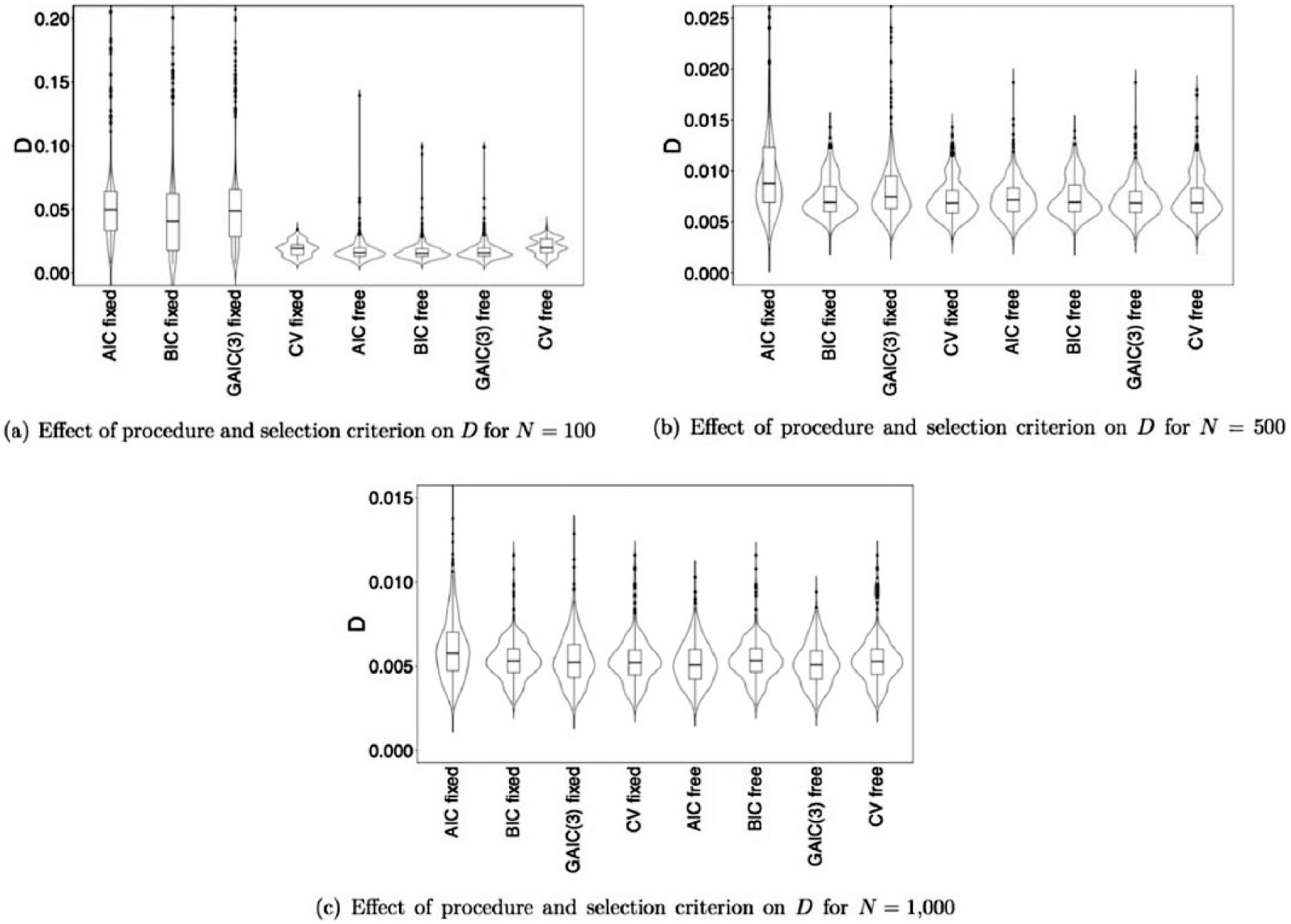
Violin plots with boxplots of the distribution of D for the eight combinations of procedure and selection criterion, for N = 100, panel (a), N = 500, panel (b), and N = 1,000, panel (c).

Data Condition and Sampling Design

We have seen in Tables 5 and 6 that all effects involving data condition and sampling design appear to be weak (η² < .02). If there are differences, Tables 2, 3, and 4 show that D becomes larger as the population data become more complex and that D is always larger for weighted sampling compared with uniform sampling (given the simplest population data condition).

Interpretation Outcome Variable D

So far, we have seen the size of the effects of procedure, sample size, selection criterion, data, and sampling design on our outcome variable D. A value of D equal to zero means that the population and model-implied distributions overlap perfectly. So, it is clear that we want the value of D to be as small as possible. However, it is not directly clear how values of D larger than zero should be interpreted. To get a better idea of this, we looked at different values of D and examined the corresponding difference in population and model-implied distributions, the difference in the functions of score against age, and the difference in percentiles.

Specifically, we considered values of D associated with the conditions in Figure 4(a). We have seen that the free order procedure in combination with the BIC on average has lower values of D than the fixed order procedure in combination with the BIC, for N = 100, uniform sampling, and the simplest population data condition (“1000”). Hence, we have inspected the practical significance of the effects. We looked at one particular replication with uniform sampling, the simplest data, the BIC, and N = 100, selecting an instance for which the D values were close to the median values found across the replications, as can be seen in Table 2.

Figure 5 shows the PDFs, panels (a), (e), and (f), and the corresponding cumulative distribution functions, panels (b), (d), and (f) for age values 8, 22, and 35. The lines represent the population model (thick line), fixed order procedure model (thin line), and the free order procedure (dashed line). It can be seen that the score distribution of the fixed order procedure generally deviates considerably and in an unrealistic way from that of the population, whereas the estimated PDFs based on the free order procedure provides more accurate results. As a result of this, the percentiles as estimated by the fixed order procedure will deviate considerably from the actual (population) percentiles for these score ranges, as can be seen in the corresponding cumulative distribution functions.

Figure 5.

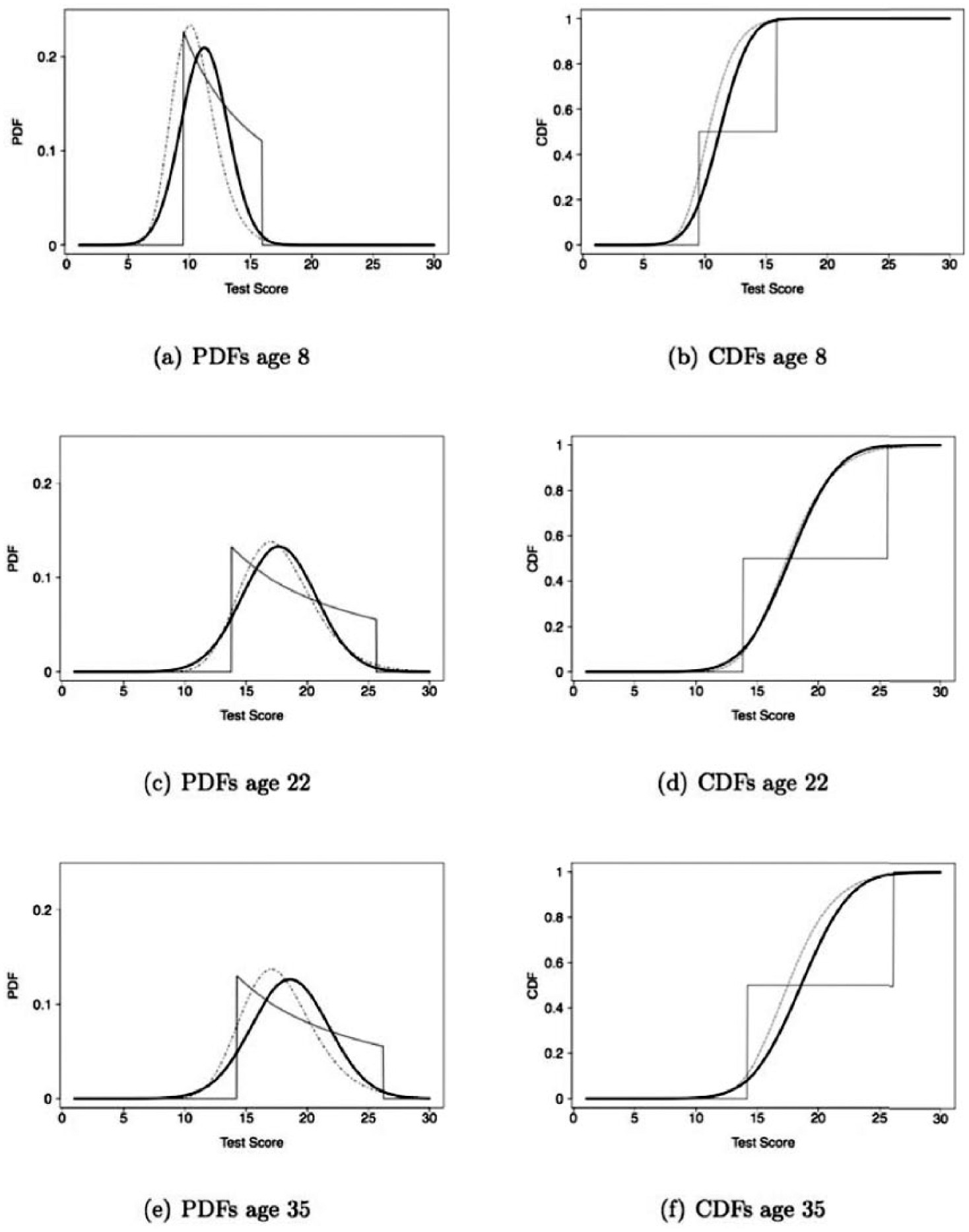
PDFs in panels (a), (e), and (f), and CDFs in panels (b), (d), and (f) for difference age values in each row (8, 22, or 35 years).

Figure 6 shows the relationship between µ and age, for uniform sampling, the simplest data condition, the BIC, and N = 100. While the functions as estimated by both procedures fluctuate around the population function line, the function from the free order procedure generally stays closer to the population function than the function of the fixed order procedure.

Figure 6.

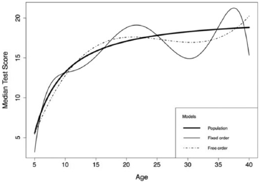
Relationships between the median test score and age.

Bias and Variance

We have separated our outcome measure D in a bias and variance component. The tables with results can be found in the supplementary material. Tables S1, S2, and S3 show the median and SD for the bias in each condition, for sample size N = 100, 500, and 1,000, respectively. The bias was in general very small: We had to multiply the results by 1,000 to see some differences. We see that bias increases as N decreases and/or as the population data become more complex. The bias seems to be lower for the free order procedure compared with the fixed order procedure when N = 100. However, this difference disappears when N = 500 or 1,000. Sampling design does not seem to have an effect on the bias. Bias seems in general to be lower for the GAIC conditions compared with cross-validation. Tables S4, S5, and S6 show the median and SD for the variance in each condition, for sample size N = 100, 500, and 1,000, respectively. Like the bias, the variance increases as N decreases and as the population data become more complex. For N = 100, the variance is lower for the free order procedure compared with the fixed order procedure when one of the GAIC is used as selection criterion. However, the variance of the free order procedure is higher than the fixed order procedure when cross-validation is used. For N = 500 and 1,000, the differences become very small or even nonexistent. As with bias, the sampling design does not seem to have an effect on the variance.

Estimating Norms With GAMLSS: The SON-R 6-40

The data of the SON-R 6-40 (Tellegen & Laros, 2014) were used to illustrate the use of the fixed and free order stepwise model selection procedure in combination with the BIC as model selection criterion. The sample size of the SON-R 6-40 data is 1,933. A weighted sampling design, different from the one in our simulation study, was used: The number of observations gets smaller as age gets larger. For example, there are 717 observations between 6- and 11-year-olds, and only 66 observations between 35- and 40-year-olds.

Figure 7 shows the observed total scores in the sample as a function of age (in years), and the resulting estimated centile curves, for the fixed order and free order procedure. The difference in centile curves between the fixed order and free order procedure is very small for age values between 5 and 35, except for the lowest centile curves. For both procedures, the median test score steeply increases for age values between 6 and about 17. After that, the median test score remains quite constant. For age values between 35 and 40, the centile curves differ quite a lot between the two procedures: The centile curves below the 50th percentile increase for the fixed order procedure, while they decrease for the free order procedure. This difference is probably due to the very small number of observations within this age range.

Figure 7.

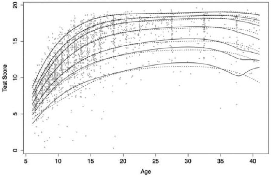
The observations (gray squares) and the estimated model-implied percentiles (5, 15, 25, 50, 75, 85, 95) for the total test scores on the SON-R 6-40 as a function of age (in years).

To further illustrate the estimated model, Figure 8 shows the PDFs for 8-year-olds, 22-year-olds, and 35-year-olds. As our simulation study clearly showed that the free order procedure performed about equal to or better than the fixed order procedure, we only show the PDFs for the free order procedure. The figures do not only show a clear difference in median total test score but also in terms of shape: The PDF for 8-year-olds is quite symmetrical and peaked, while the PDFs for the 22- and 35-year-olds are very negatively skewed. As soon as you have these distributions, the norms can be determined for each combination of age value and test score. For instance, for an 8-year-old with a total score of 10, the percentile is 66. For a 35-year-old with the same score, the percentile is 3. As the percentiles can be determined for each age value, this can be done for the exact age of the test taker.

Figure 8.

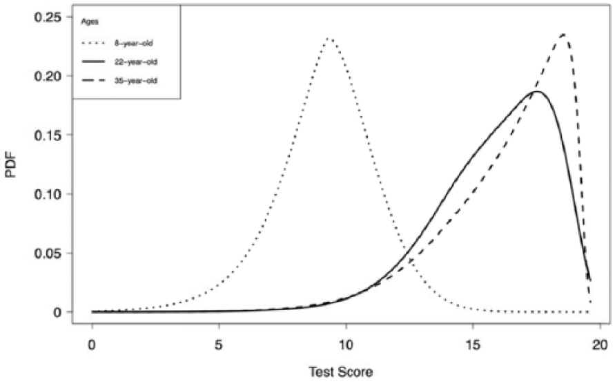
The fitted PDFs of the total score of the SON-R 6-40 test, for 8-, 22-, and 35-year-olds (dotted, solid, and dashed line, respectively).

To facilitate the calculation of the norms, we have implemented our model selection procedure and the determination of the resulting percentiles in R code. The only thing the user has to do is to specify the data set (including test scores and a predictor, like age) and the values of the predictor value and test score for which to determine the percentiles. This R code can be found as supplementary material.

Discussion

In this study, we investigated the performance in accuracy of estimating norms for different stepwise model selection procedures (i.e., fixed order and free order), model selection criteria, that is, AIC, BIC, GAIC(3), and cross-validation, sample sizes (N = 100, 500, and 1,000), sampling design, and population data models, varying in complexity. We have found a large effect of sample size: The norms are estimated more accurately as sample size increases, regardless of the other factors. The relationship between D and N was nonlinear: The decrease in D was larger when N increased from 100 to 500 compared with when N increased from 500 to 1,000. In our study, it appeared that the norms are estimated accurately when the sample size is large (i.e., N = 500 or 1,000), irrespective of procedure, model selection criterion, sampling design, and complexity of the data. However, it does matter which procedure and which model selection criterion is chosen when the sample size is small (i.e., N = 100). Our own developed stepwise model selection procedure, the free order procedure, outperforms the fixed order procedure when used in combination with one of the GAIC. In terms of median D value, the GAIC outperforms cross-validation, regardless of the procedure used. Moreover, cross-validation often resulted in nonconvergence and required way more computational effort and time to compute than the other criteria. We even had to limit the model search area for the fixed order procedure in combination with cross-validation to increase the probability of convergence. For N = 100, the best combination of procedure and selection criterion is the free order procedure with one of the GAIC. As the free order procedure required the lowest sample size for the same performance, it is the most efficient model selection procedure.

We have seen that the difference between the fixed and free order procedure when N = 100 has practical significance, as the estimated percentiles for the fixed order procedure deviated a lot from the actual (population) percentiles, while the percentiles for the free order procedure were much more similar to the actual ones. As the values of D were even much smaller for N = 500 and 1,000 compared with those of the free order procedure with N = 100, we are confident that the estimation of norms is accurate in those conditions with larger sample sizes. Even though we expected the simple data conditions to outperform the more complex ones, there seemed to be only small differences in the accuracy of estimating norms across population data models. This makes us confident that similar results will be found for data different from the data we simulated in this study. Other data might contain different, possibly even more difficult, relationships. Interestingly, contrary to our expectations, we did not find an effect of sampling design on the accuracy of estimating norms. The weighted sampling did not outperform uniform sampling. Moreover, we did not find the expected interaction effect between N and sampling design.

In addition to the accuracy, D, we separated this measure into a variance and bias component. We found that both variance and bias increased as N decreased and as the data became more complex. For N = 100, there was also a considerable effect of procedure and selection criterion. It is interesting that sample size has an effect on bias. A reviewer wondered whether this is caused by too simple models chosen when the sample size is small. Inspection of the chosen polynomial degrees in the most complex data condition revealed that indeed more complex models were chosen as sample size was larger. We believe it is interesting to investigate this further in future research. Note that we generated the population data without using polynomials, which makes it impossible to compare the chosen polynomial degrees with the “true” degrees.

A strength of this study is that we used empirical data in combination with simulated data. We based the generation of the data on the SON-R 6-40 data (Tellegen & Laros, 2014). We tried to make the difference between the data conditions as large as possible, while keeping them realistic. In addition, we illustrated our method with the SON-R 6-40 data.

The scope of possible terms to include in the models for the distributional parameters was broader for the free order procedure (i.e., intercept to polynomial with degree 20) than for the fixed order procedure (i.e., intercept to polynomial with degree 7). This might have given the free order procedure an unfair advantage over the fixed order procedure. However, inspection of the selected terms for the free order procedure shows that polynomials of degree 8 and higher are rarely chosen and that these selected models perform relatively bad.

Future Research

We have two suggestions for future research. First, it is interesting to look at models with multiple predictors. In our study, we included one predictor, namely age. We have seen in practice that additional demographic characteristics, like gender, are used as predictors. We have no reason to expect that the results of the present study differ when more predictors would be included. However, we believe it is interesting to investigate in which way models need to be selected for the different predictors. Should the parameters be updated subsequently for the different predictors or at the same time? The free order procedure does not allow for multiple predictors yet. As this procedure in general outperformed the fixed order procedure, it is important that this procedure allows for multiple predictors as well.

Second, it is very important that can be determined how large the norming sample needs to be. We have seen that in our study N = 1,000 (and perhaps N = 500) was enough to have good estimation of the norms, regardless of the complexity of the data and the choice of procedure, model selection criterion, and sampling design. However, this does not mean that N = 1,000 is large enough in every norming study. Usually, it is very difficult to determine whether your sample size is large enough. Oosterhuis et al. (2016) provided sample size requirements for regression-based norming, but they assumed normality of the score distributions conditional on gender and age. Hence, our suggestion for future research is to determine sample size requirements for non-normal distributions.

Practical Implications

We have seen that the choice of procedure, model selection, and sampling design does not matter when the sample size is large enough. As the sample size is often an issue in practice, it is interesting to consider the factors that we have shown to perform better than others for smaller sample sizes. Our study resulted in clear recommendations regarding this: It is best to use the free order procedure in combination with one of the GAIC. The BIC seemed to perform slightly better than the others, which is why we recommend to use this criterion. Even though we did not find an effect of sampling design, we still have a recommendation regarding this factor. Because this is a simulation study, we have the luxury of knowing the true relationship between age and µ, even before having to determine how many people of a particular age to include in the norming sample. In practice, however, this function has to be estimated with the norming sample. A general estimate of the relationship between µ and age can be based on a preliminary sample and/or the results of previous (versions of) tests. However, our results showed that even knowing this relationship was not helpful. The two sampling conditions did not seem to differ. If they did, uniform sampling even slightly outperformed weighted sampling. Because of this finding and the fact that weighted sampling is more difficult to carry out, we advise to use uniform sampling. Moreover, as a reviewer pointed out, it might even be dangerous to use weighted sampling based on change in median test score only when other distributional parameters depend on the predictor(s) for certain (other) ranges.

When the free order procedure is applied, it is possible that the model cannot be estimated. We have seen that this problem is most likely to occur for complex data sets in combination with a small number of observations. Hence, if this occurs in practice, the sample size is probably too small.

Finally, there are fewer observations near the boundaries of the data to support the model. On top of this, polynomials have notorious tail behavior, which makes the model very untrustworthy near the ends of the data, but also outside the range of the data (Hastie et al., 2009). Hence, we advise to make the age range of the people in the norming sampling big enough, even somewhat bigger than the age range you want to develop norms for. In addition, statements about age ranges outside those in your norming sample (i.e., extrapolation) should be avoided.