
Abstract
Some places are more likely than others to experience crime. These locations are typically small and usually have a high consistency of crime over time (Andresen et al., 2017; Weisburd, 2015; Weisburd et al., 2004). Preventing crime by identifying these hotspots and directing police there is effectful in reducing crime (see e.g., Braga et al., 2019). This policing method, however, is dependent on finding these hotspots. To prevent crime, one first needs to identify future crime locations with some level of accuracy.
A unique combination of risk factors at the place, and neighborhood-level can generate a context both inviting and upholding opportunities for criminal behavior (e.g., Brantingham & Brantingham, 1995). Certain place features in the environment such as bars, schools, bus stops, and restaurants can create opportunities by generating and attracting crime. To some extent, this is likely due to crime opportunities arising at places where lots of people congregate (see, e.g., Gerell, 2021). The influence of these place-features on crime can furthermore be affected by neighborhood characteristics such as concentrated disadvantage (see Shaw & McKay, 1969; Tillyer et al., 2021), and collective efficacy (Gerell, 2018; Sampson et al., 1997).
Interconnectedly, there are different ways of identifying crime hotspots. Depending on a theoretical standpoint, different data types and analytical approaches are required. This raises the question of how much data is needed for accurate practical forecasting. In this study, we aimed to assess how the predictive accuracy differs when using individual factors (e.g., prior crime, place attributes, ambient population, community structural, and social characteristics), in isolation and when combined in forecasting various types of violent and property crimes.
To aid this endeavor, a very crude version of Risk Terrain Modeling (RTM), using multilevel negative binomial regression, Prediction Accuracy Index (PAI), and Prediction Efficacy Index (PEI*) is used. Together, these methodologies will not only enable a comprehensive understanding of the relationship between crime generators and crime but also facilitate practical and effective communication of the findings.
Identifying Hotspots of Crime
Two approaches to identifying hotspots of crime are retrospective hotspot maps and methods based on regression (Reinhart & Greenhouse, 2018; Wheeler & Steenbeek, 2020). In retrospective hotspot mapping crime history is used to forecast crime (Groff & La Vigne, 2002). Simply, where a lot of crime has been in the past, there will be a lot of crime in the future (see, e.g., Braga et al., 2019; Chainey et al., 2008; Wheeler & Steenbeek, 2020). Crime history is the sole predictor.
Another option is to use different crime generators regressed onto crime. Related theories such as crime pattern theory (CPT; Brantingham & Brantingham, 1993) and the routine activity theory (Cohen & Felson, 1979) are used to explain why both violence and property crime occur at the hotspots and what crime generators are related to these places. Crime, according to CPT, depends much on the context of the specific location (Brantingham & Brantingham, 1993, 1995). Places with many people are often referred to as crime generators. People are there to go about their daily business, not to commit crimes. However, an opportunity and/or situation to commit a crime might present itself for crime-prone people. The sheer concentration of people and potential goods is what generates crime. Examples of crime generators are shopping malls and districts, entertainment districts, and travel nodes, for example, bus- and train stops.
Crime attractors according to CPT, on the other hand, are environments and situations where it is known to be conducive to commit a crime. It is places and times where motivated offenders are drawn due to the known opportunity to commit crime, such as open drug markets, areas with prostitutes, large unattended parking lots, shopping malls, and entertainment districts. Some types of places could be both crime generators and crime attractors such as a shopping mall or bar. Offender motivation is really what determines whether a place is a crime generator or a crime attractor. Common crime generators in research, also used in the current study are the presence and amount of restaurants (Groff & Lockwood, 2014), bars (Kennedy et al., 2011; Wheeler, 2019), schools (Bernasco & Block, 2011; Kennedy et al., 2016), public transit (Bernasco & Block, 2011; Gerell, 2018), ATMs (Haberman & Ratcliffe, 2015), different types of land use such as apartment buildings and parks (see, e.g., Haberman et al., 2013; Wheeler & Steenbeek, 2020). Ambient population (Gerell, 2021; Malleson & Andresen, 2016) is another variable used.
The structural and social patterns of the broader neighborhood can also aid in explaining/predicting crime. The social disorganization theory posits that a high population turnover, concentrated disadvantage, and ethnic heterogeneity affect disorder (Shaw & Mckay, 1969 based on ideas by Burgess, 1925; Park, 1925a, 1925b, developed by Kornhouser, 1978). This relationship between structural neighborhood characteristics and deviance is mediated by community cohesion and social control. One example being the inability of residents to organize against disorderly behavior, due to a lack of cohesion because residents continually move in and out of the neighborhood. In short, places that are more socially disorganized will have more crime. Places with more social organization will have less crime.
Contemporary elaboration of the social disorganization theory (Kornhouser, 1978; Shaw & McKay, 1969), with the inclusion of informal social control, has led to the collective efficacy theory (Sampson & Groves, 1989; Sampson et al., 1997). Strong cohesion and informal control in the neighborhood will lead to high collective efficacy and likely to less crime in the neighborhood. Neighborhood-level characteristics can hence also be regressed into crime. Neighborhoods with higher collective efficacy, that has higher cohesion, trust, and an expectation to act for the commonweal, show lower levels of crime than those with low collective efficacy (see, e.g., Sampson & Wikström, 2008; Sampson et al., 1997; Wikström et al., 2012). Collective efficacy is affected by neighborhood concentrated disadvantage, population heterogeneity and residential instability, the three pillars of social disorganization (Sampson et al., 1997). The concentrated disadvantage is strongly associated with collective efficacy, but can also influence crime through other mechanisms, such as young people in socially disorganized neighborhoods hanging around street corners (Sampson & Groves, 1989). The context of neighborhood concentrated disadvantage might exacerbate crime in smaller locations with place-level crime generators (see, e.g., Tillyer et al., 2021). There are hence likely interactions between these different place- and neighborhood variables. For example, a bus stop (place variable) might be more prone to violence in an area where guardianship is low due to low collective efficacy (neighborhood variable; Gerell, 2018).
One common method using regression and used by practitioners is RTM (see Caplan et al., 2015). RTM is a proprietary technique and uses the tool RTMDx (Caplan et al., 2013), a for-profit software application, to ease the process of analysis by automation for practitioners. In RTM, potential crime hotspots are identified using environmental variables. A city is first divided into a grid. Then theoretically and practically important crime generators (such as the presence of an ATM, bar, transportation node or not) for the specified crime type are calculated per grid cell. In RTMDx this is done with an elastic net penalized Poisson regression, with all variables represented by their proximity/density at different spatial scales. Hence multiple operationalizations of the independent variables are used. After the regularizing of the coefficients, which is done to get a smaller set of final variables included in the model, a bidirectional stepwise regression model starting from a null model tests the different remaining variables and compares the BIC scores to find the right version (lowest BIC-score) of a variable. Certain combinations of risk factors will after regression be found to be key in explaining future crimes (according to Caplan et al., 2011), and a combined risk score is calculated. When risk values according to the risk composite have been assigned to each grid cell, you have a risk terrain map (see Caplan et al., 2015). This map tells us whether a particular place is a place with a high risk of crime.
Study Relevance
Looking at the state of research today, to forecast crime properly in microplaces, one should use different types of crime generators, at different levels (spatial scales) of explanation. The structural patterns of the overall neighborhood such as concentrated disadvantage, and collective efficacy as well as the specific patterns, dynamics, and attributes of the place within the neighborhood itself, are argued, to be considered in explanations of crime consistency (see, e.g., Hipp & Williams, 2019; Tillyer et al., 2021). The list of risk factors to include fast becomes vast. In addition, the analysis of all possible effects of the included factors on crime, as well as interaction effects (within and between levels) between these risk factors becomes quite complex. Making forecasts with large amounts of spatial data is very time-consuming, however, and can also be quite costly. The data must first be collected and then processed. Using vast amounts of spatial data also introduces a lot of decisions that need to be made by the crime analyst, usually working with time constraints. Hence, for practical purposes, we must assess if a simple crime count (simple, transparent, and functional), is effective or if more complex methods, like regression techniques that encompass all aspects of place-based theory, such as the today commonly used semiautomated RTM, offer greater accuracy. Some prior studies omitted a simple crime-counting measure in method comparisons (Caplan et al., 2011; Chainey et al., 2008; Drawve, 2016; Levine, 2008). This is problematic, as counting crimes is both simple and cheap (Groff & La Vigne, 2002; Wheeler & Steenbeek, 2020). Studies that include a simple count of crime history (Wheeler & Steenbeek, 2020), or other crime history information (Rummens & Hardyns, 2020) reveal that crime history performs quite well forecasting crime when compared to methods that include more data collection. Others do not however (Ohyama & Amemiya, 2018). Research on data requirements for crime forecasts is inconclusive. Simpler methods can however yield good results (Lee et al., 2020).
Aim
The aim of the current article was to assess how the predictive accuracy differs when using individual factors (e.g., prior crime, place attributes, ambient population, community structural, and social characteristics), in isolation and when combined in forecasting various types of violent and property crimes.
Method
The current study was based on four data sets from the municipality of Malmö in southern Sweden. First, reported crimes (crime incidents), were provided by the local police in Malmö for 2016 and 2017. Second, census data on the residents’ sociodemographic characteristics (for the year 2015) and information regarding place variables (year 2017) was provided by Malmö municipality. Third, a community survey from 2015, was provided by Malmö University. Fourth, geographical information on local bus stops and annual passengers visiting these bus stops between March 2014 and March 2015 was provided by the regional transportation company Skånetrafiken. The study was approved by the Swedish ethical review authority: #2017/479.
Research Setting
Malmö, Sweden's third-largest city (population: 331,201 in June 2017; SCB, 2017), exhibits higher crime, unemployment, foreign-born residents, and young population (Ekström et al., 2012; Malmö stad 2014; SCB, 2020) compared to the rest of Sweden. The city has 136 neighborhoods, with 104 included in the analysis (Level 2). Selection criteria included neighborhoods with a minimum of 200 residents aged 20 to 79 (January 2015), and excluded neighborhoods primarily comprising parks, harbors, and industrial zones where few people reside (Guldåker & Hallin, 2013; Ivert et al., 2013). All data has been spatially joined to a fishnet grid overlaying the Malmö municipality area, with a total of 65,594 grid cells the size of 50-m. In the same setting of Malmö, studies have shown the advantage of smaller 50-m micro-place geographies for analyzing arson-related characteristics (Gerell, 2017). This smaller cell size was also effective in another test of a crude RTM in Malmö (Gerell, 2018). When forecasting violent crime using crime history alone (Camacho-Doyle et al., 2021), a 50-m cell size resulted in a PAI-value of 237 in 2017, compared to 66.84 using a 100-m cell size. Similarly, smaller cell sizes around 50 m have been utilized in other settings (Kennedy et al., 2011; Wheeler & Steenbeek, 2020).
Data
Dependent Variables
Crime Count
Police recorded crimes (point data), on public environment assault, street robberies, property damage, theft, vehicle theft, illegal fire setting, and residential burglary, from January to December 2017, aggregated to grid-cells were used as the dependent variables. The crime points were spatially joined with intersect using ArcMap 10.6.1 to the 65,594 grid cells in the fishnet grid. Reported crimes in Sweden are like U.S. crime incidents/events, not calls for service. The classification of crime is based on offence codes, which include information about the type of offence and, for some crime types, additional contextual information. Assault for instance has specific offence codes for whether the perpetrator has a relation to the victim, whether the victim is an adult, the victim gender, whether it was outdoors or indoors, and whether it was normal or aggravated assault.
Independent variables
A weakness in the analysis is that some of the independent variables are from 2014 to 2015 rather than from 2016. While most variables will tend to be fairly stable over time, this may have some impact on the reliability of our results.
Crime data
Police recorded crimes (identical to the dependent variables) but from January to December 2016, aggregated to grid cells were used to measure crime history. Within-crime type analysis was done. Hence, assault in 2016 was used only to forecast assault in 2017 and property damage in 2016 was only used to forecast property damage in 2017.
Place variables
The geographic location of restaurants, bars, ATMs, schools, preschools, bus stops, parks, town squares, sports fields, small house units, apartment building units, and vacation homes were used for the RTM. For the point data (restaurants, bars, ATMs, schools, preschools, and bus stops) kernel density estimations (KDEs) with 50-m pixel size, 500-m radius were used to assign cells a value for each risk factor in line with prior studies in the city (Gerell, 2018). The KDE was used to smooth out the effect of a place variable, as for instance a bar likely affects not just the exact location where it is, but also nearby locations. In using this smoothing effect, we also in effect model something similar to a spatially lagged version of our independent place variables, which has been shown to be of importance to crime outcomes (Haberman & Ratcliffe, 2015). This was done in ArcMap 10.6.1. The processing extent was set to the municipal boundaries. The KDE values were then spatially joined using intersect to the fishnet grid laid over the Malmö municipality area.
The building and other landscape polygons were spatially joined with intersect to the fishnet grid. A pixel in the grid was assigned 1 for a variable if a polygon measuring that variable (for instance, a park) intersected the pixel. Like RTM, the geographic place variables that revealed a positive and significant relationship with each respective outcome variable (e.g., assault, robbery, property damage, etc.) were standardized as Z-scores, weighted according to the regression coefficient, and summed into an index.
Ambient Population
As a proxy of the ambient population at places, geocoded point data of local public bus stops and the annual number of passengers boarding each stop were used. A KDE with 50-m pixel size, and 500-m radius populated by the total amount of passengers boarding each stop were used to assign all grid cells a value. This measure of ambient population is imperfect but yields a reasonable proxy measurement for where lots of people move since bus stops are planned to capture flows of people. The ambient population tended to have a negative relationship with crime after other variables were controlled for and was therefore reversed before being indexed. The higher the value, the less ambient population at that location.
Collective Efficacy
Collective efficacy was measured using data from a community mail survey, from the year 2015 (MCS, 2016). The scale is a Swedish language version of that used in Wikström et al. (2012). A minimum of 10 responses per neighborhood was required, a threshold also noted in prior research (Steenbeek & Hipp, 2011). The response rate was 40%. The collective efficacy index (α = .940) was created using ten Likert-type items measuring cohesion and informal control. The cohesion and informal control subscales have previously been used in research (Gerell & Kronkvist, 2017; Sampson et al., 1997; Wikström et al., 2012). Data was aggregated to neighborhood-level (104 neighborhoods) and standardized as Z-scores before being indexed. In cases of missing data, any respondent with responses on less than three items (out of five) relating to cohesion or informal control was excluded (n = 93 respondents).
Concentrated Disadvantage
Neighborhood concentrated disadvantage (Gerell & Kronkvist, 2017; Sampson et al., 1997) was measured using six variables (α = .925) standardized as Z-scores, in an index. Median income (reverse-coded). The proportion of unemployment including residents aged 20–64, in 2015. Proportion of public assistance from 2016. To protect residents’ integrity no data was provided for neighborhoods with few households receiving assistance. In this study, these (34) neighborhoods have therefore been recorded to have no households on public assistance. The proportion of single-parent households was defined as the proportion of households with a single adult living with at least one child of blood relation, in 2015. Car ownership in 2015 (reverse-coded). The proportion of foreign-born individuals in 2015, to capture the concept of ethnicity.
Age Structure
As a proxy for the amount of young people hanging around street corners (Sampson & Groves, 1989), the proportion of adults in comparison to young people was calculated as the ratio between adults, everybody 20 years and over and child, everybody 19 years and under, in 2015. A higher ratio would imply more adults per young person, which in turn would be expected to be associated with less crime.
Analysis
Multilevel negative binomial regressions were performed in R 4.0.3 using the MASS-package (Venables & Ripley, 2002) and the lme4-package (Bates et al., 2015). These multilevel models were used to analyze the contribution of microplace (Level 1 in the models, i.e., grid cells), and neighborhood-level variables (Level 2 in the models) simultaneously, on grid-cells with crime in 2017. To be consistent with RTM, no cross-level, nor within-level interaction terms are included in the model. The dependent variables, crime counts, normally exhibit negative skewness, and overdispersion (see Hilbe, 2011). To address this, we employed negative binomial and Poisson regression models and ran boundary likelihood ratio tests for overdispersion, following Hilbe (2011, p. 178). The results, assessed using the lmtest package (Zeileis & Hothorn, 2002) and chi-squared values, confirmed the appropriateness of negative binomial models for all crime types. To avoid multicollinearity, the Variance Inflation Factor (VIF) was tested for all independent variables, with the performance package (Lüdecke et al., 2021). Bars and restaurants revealed a VIF of >5 and were therefore combined.
A crude RTM was first performed for all crime types (Table S1 in the supplemental material). 1 The place variables were run separately to get a combined RTM index for each crime type. Variables that revealed a positive and significant relationship with the respective crime type were weighted according to the regression coefficient and summed into an index. Then several regressions were run (Table S2 in the supplemental material), for each crime type separately. In Model 1, crime history (grid cells with crime count in 2016) was run for each crime type respectively. In Model 2 the RTM was added. In Model 3, the ambient population was added. In Model 4, the neighborhood-level variables (Level 2) collective efficacy, concentrated disadvantage, and age ratio were added. For each crime type, the significant coefficients (p < .05) from Models 2, 3, and 4 in the regression (Table S2 in the supplemental material), were weighted and combined to get the composite scores, 2 similar to Gerell (2018). This was done to get overarching indexes, to be able to calculate PAI/PEI*, with risk factors at different levels in each grid cell for comparison.
PAI values were calculated for each significant index. This was done to see how the prediction accuracy increased or decreased with the addition of variables. With the PAI value (proposed by Chainey et al., 2008) you examine the accuracy in finding the hotspot, by comparing the hit rate (how much crime you can forecast in the hotspot compared to the total amount of crime in the study area) to the area of the hotspot and of the whole study area. PEI* values (based on Hunt, 2016, introduced at the 2017 National Institute of Justice (NIJ) Real-Time Crime Forecasting Challenge) were also calculated. PEI*-values go from zero to one, where zero means that no hotspot was forecasted at the predicted time. A value of one indicates that the model accurately forecasted the actual hotspots. Values below 1 means that the model could have done better.
For easy comparison of the different methods, the hotspots were identified by choosing the top grid cells predicted as hotspots (1, 10, 50, 100, and 500 cells) of the whole study area, up to 1% (about 656 cells) of the study area. This is like the NIJ predictive policing challenge (see, e.g., Lee et al., 2020; Mohler & Porter, 2018), rather than using the grid-cells with a density value of two standard deviations above the mean as is otherwise common (Chainey et al., 2008; Drawve, 2016). Furthermore, multiple thresholds for the PAI/PEI*-values for assault and property damage can be viewed in Figure 2. This was done to show how the different values are affected by the size of the area included for calculation.
Results
Crime history was significant (p < .001) when forecasting all crime types, all other variables controlled for. As can be seen in Figure 1 and looking at the estimated Incidence Rate Ratio (IRR) from the negative binomial regression model, the results differ for different crime types. There is a large amount of variance across crime types. In short, however, where there has been crime in the past, the risk for future crime is higher. As also can be seen in Figure 1, when compared to places that do not have the combined place characteristics, RTM was significant (p < .001) when forecasting all crime types, all other variables controlled for. In short, where characteristics conducive for crime congregate, the risk for crime is higher. RTM generally produced higher IRR scores than crime history alone.
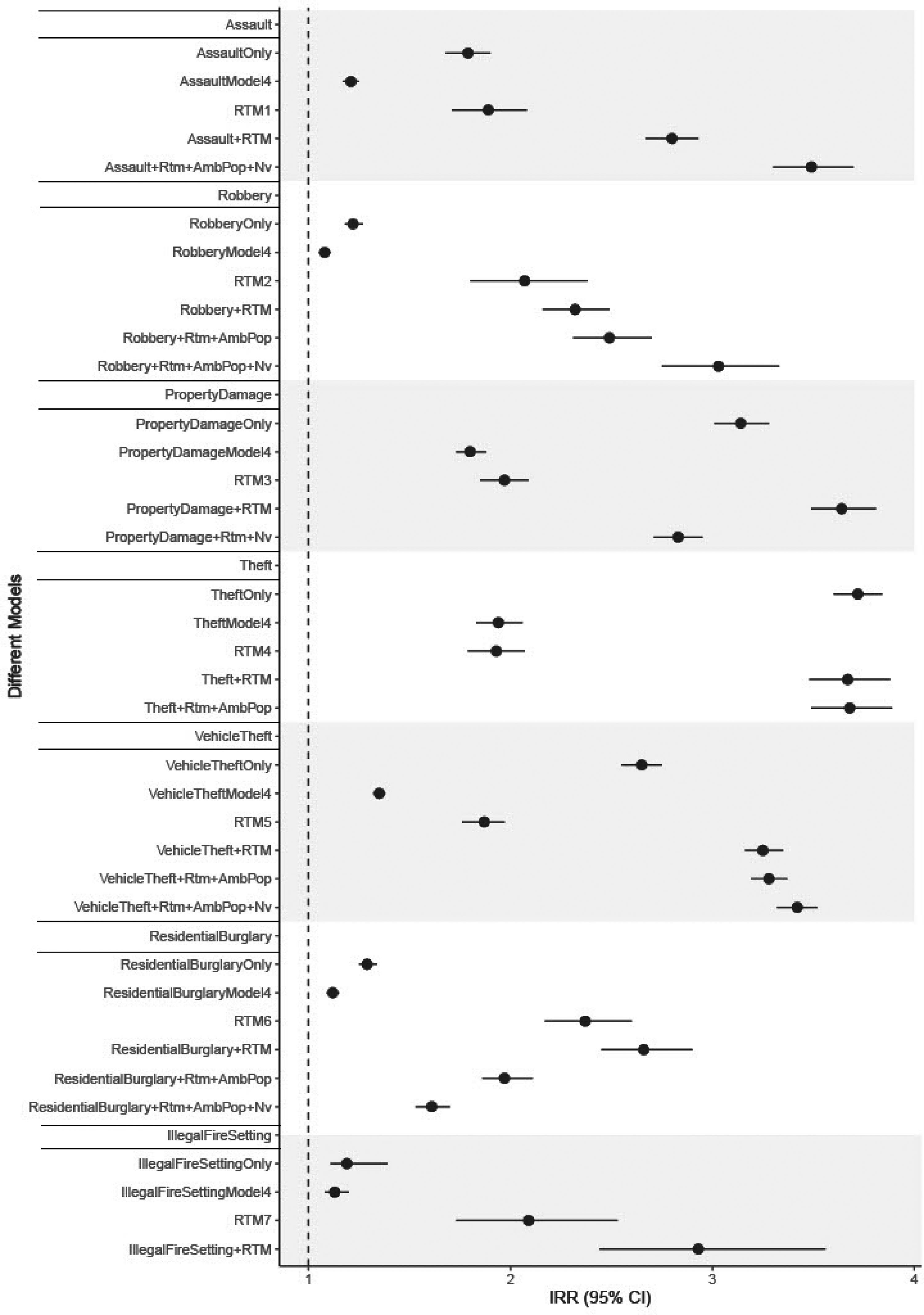
Forest plot for the forecast models accross all crime types.
To see if combining prior crime with the RTM as well as if adding ambient population and neighborhood-level characteristics increase the accuracy, compared to simply looking at crime history, the significant coefficients from Models 2 and 4 in the regression (Table S2 in the supplemental material), were combined to get composite scores. Compared to places that do not have the combined RTM and prior crime as well as the combined prior crime, place-, and neighborhood characteristics, the composite scores resulted in higher IRR for almost all crime types (Figure 1). For example, there was 3.49 times the risk for assault, with the combination of crime history, RTM, neighborhood concentrated disadvantage, low collective efficacy, and more adults per young people, compared to places that do not have the same combination. For robbery, there was 3.02 times the risk, and for vehicle theft 3.42 times the risk with the combination of crime history, RTM, less ambient population, and low collective efficacy compared to places that do not have the same combination. Furthermore, there was 3.56 times the risk for property damage with the combination of crime history, RTM, and low collective efficacy compared to places that do not have the same combination. For illegal fire settings there was 2.93 times the risk and residential burglary 2.95 times the risk with the combination of crime history and RTM compared to places that do not have the same combination. For theft, crime history alone reached the highest IRR (3.72). In short, combining important variables increased the accuracy for all crime types except for theft, when looking at IRR.
Table 1 displays the estimated PAI-values (with a number of predicted crimes in that area) as well as the PEI*-values for all crime types, and for all model forecasts: crime history, RTM, RTM combined with crime history, RTM combined with crime history and ambient population and lastly RTM combined with crime history, ambient population, and neighborhood-level data across six different fixed thresholds. RTM alone performs the worst out of all models when it comes to PAI/PEI*. However, when combined with crime history it performs quite well. Generally, combining more data to forecast all different types of crime performs well, but does not outperform simply using prior crime counts as the forecast. Looking at the PAI/PEI*-values, for robbery, vehicle theft and illegal fire setting, all included models (except for RTM alone) rendered similar PAI/PEI*-values at least in the top hotspots. Crime history renders the highest PAI/PEI*-values when increasing the number of vehicle theft hotspots. For residential burglary and theft, however, crime history alone generally rendered the highest PAI/PEI*-values across thresholds.
Accuracy Metrics Across Six Thresholds for Each of the Forecast Models.
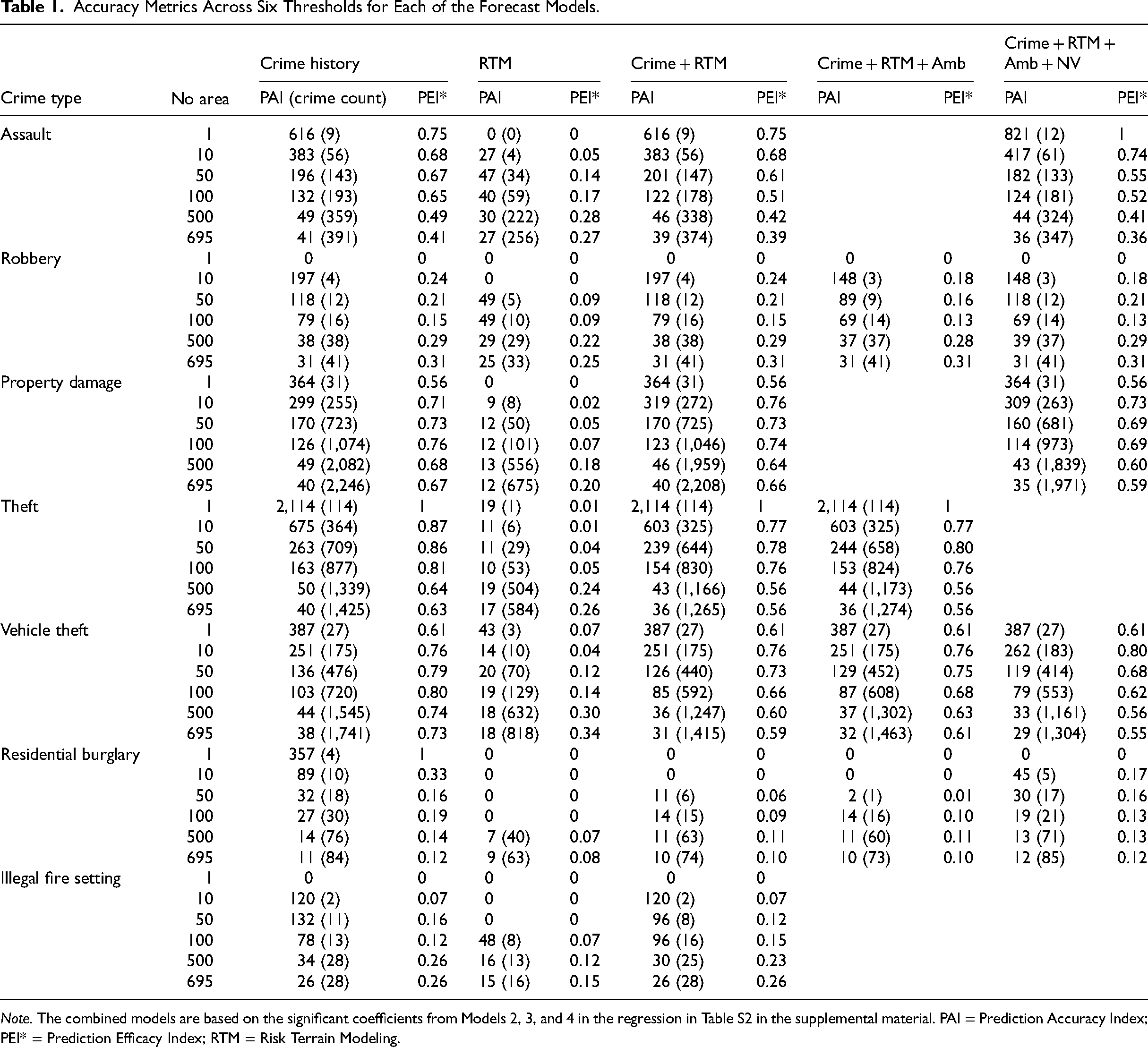
Note. The combined models are based on the significant coefficients from Models 2, 3, and 4 in the regression in Table S2 in the supplemental material. PAI = Prediction Accuracy Index; PEI* = Prediction Efficacy Index; RTM = Risk Terrain Modeling.
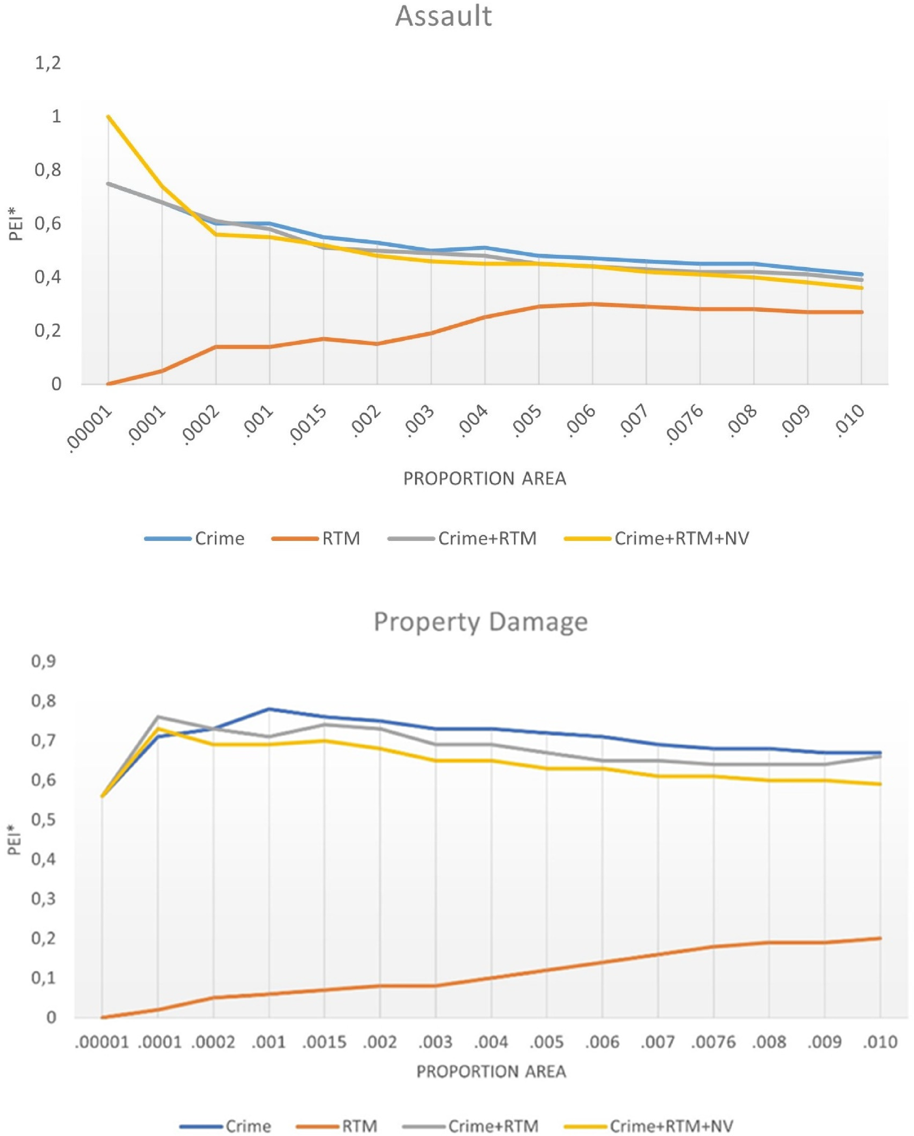
Figure 2 displays the PAI/PEI*-values for assault and property damage across multiple thresholds, up to 1% of the study area. For the top 10 hotspots for assault and property damage, a combination of all significant coefficients and a combination of crime history and RTM reached the highest PAI/PEI*-values, respectively. For all other cut-offs, all models (except RTM) have a similar accuracy. The PEI*-values for assault and property damage show that all variables combined in the top hotspots capture about 74% of the total assault count compared to the best possible forecast. RTM combined with crime history captures about 76% of the total property damage compared to the best possible forecast. Crime history alone (68% and 71%, respectively) or different combinations is an improvement over RTM alone, which only captures around 0–27% of the same proportion of crimes. In short, for most crime types and when both accuracy and efficiency are considered, crime history alone generally renders similar forecasts to models that include more data, when taking the geographical area into account.
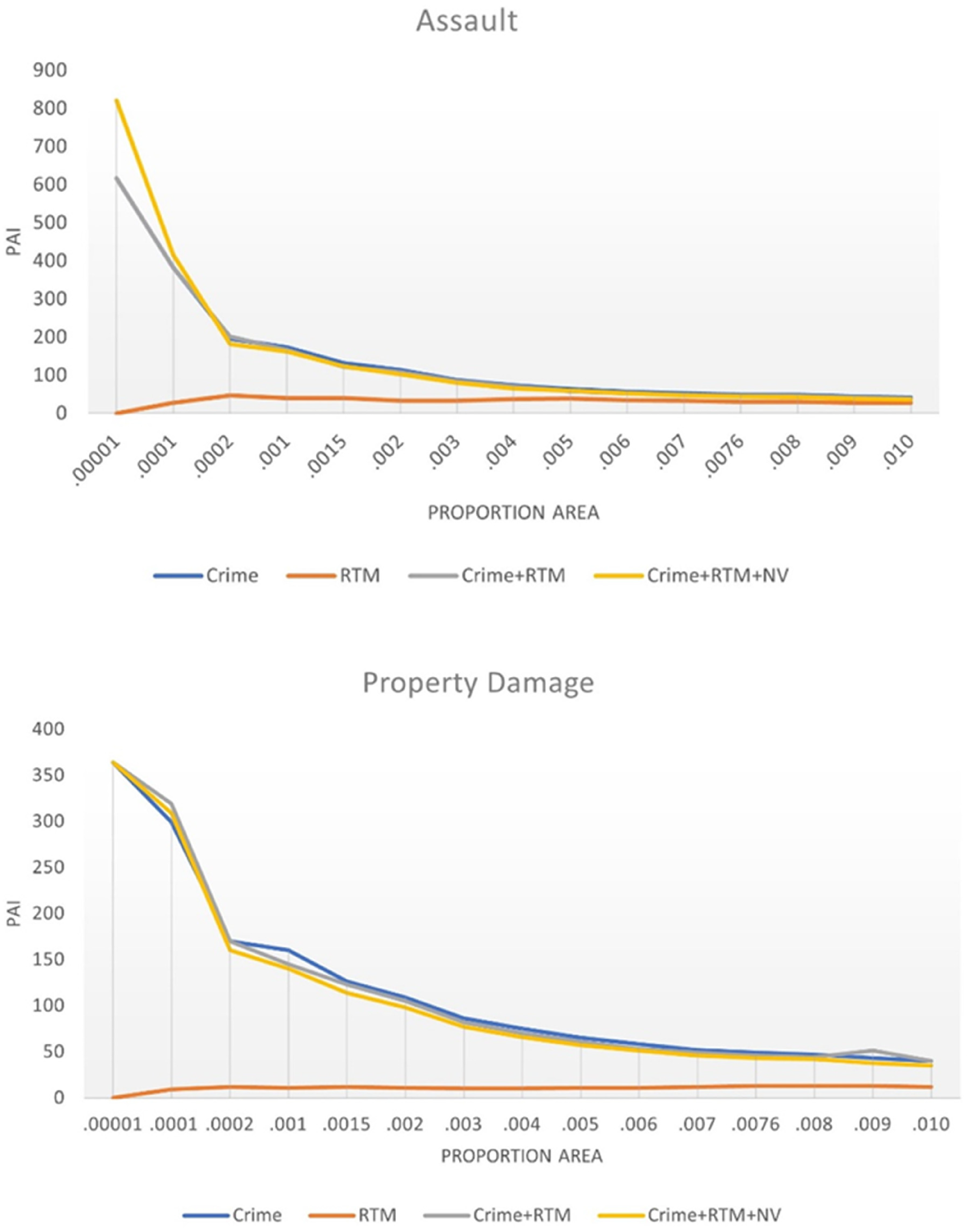
Accuracy metrics across multiple thresholds for assault and property damage for each of the forecast models.
Discussion
Widespread use of advanced methods in practice may take a few years to become feasible. Thus, it is valid to establish the accuracy and efficiency of simple methods for practical purposes. Some prior studies have neglected a measure of simply counting crimes when comparing forecasting methods (Caplan et al., 2011; Chainey et al., 2008; Drawve, 2016; Levine, 2008). This is a drawback, as counting crimes is simple and cost-effective for practitioners (Camacho-Doyle et al., 2021; Groff & La Vigne, 2002). Standard regression techniques that incorporate all elements of place-based theory, like RTM, are used in practice today and they require extensive data collection. We compared simply counting past crimes for different types of violent and property crimes, with a crude version of RTM, where we also added neighborhood-level data and ambient population.
The results showed that a combination of crime history, RTM and important neighborhood characteristics worked best for most crime types. In the top 50 hotspots (less than 0.1% of places) and using the top forecast model for each crime type, 15% of assaults, 9% of robberies, 13% of property damage, 20% of theft, 10% of vehicle theft, 10% illegal fire setting, were forecast in 2017. Only 3% of residential burglaries were forecast. This is consistent with the research on RTM, that place characteristics joined with crime history render better forecasts than RTM and crime history alone (see, e.g., Caplan et al., 2013, 2020).
However, a distinctive result across several crime types was that a simple count of past crimes renders similar forecasts to methods that require additional data collection. The analysis done by Wheeler & Steenbeek (2020) supports our argument that simple crime counts play an important role in spatial analysis. They also found that counts of prior crime had more predictive accuracy than more complicated models, including RTM. When looking at the top 10 hotspots for assault, including all variables contributes to a better forecast (for instance, 6.4% of assaults forecast vs. 5.8% using crime history alone). For assaults, this means that considering a higher concentration of town squares, bars, restaurants, ATMs, bus stops, schools, and rental apartments in areas with a higher concentrated disadvantage, lower collective efficacy, more adults per young people and history of assaults implies 0.6% (a 10% improvement) better forecast than using crime history alone.
These results might speak in favor of more simple methods, such as simply looking at crime history for certain crime types, as it is more cost-effective, transparent, and functional, for practical forecast purposes. Neighborhood-level variables did not increase the prediction accuracy substantially for any crime type except the top 10 hotspots for assault. This result contradicts findings from some recent studies (see, e.g., Tillyer et al., 2021; Weisburd et al., 2021). However, collective efficacy was measured at a neighborhood-level in the current study, as compared to the street level in the previous study (Weisburd et al., 2021). Collective efficacy might increase prediction accuracy when measured at the street level, considering microlevel social relations (Weisburd et al., 2014). Furthermore, to keep in line with an RTM method, no interaction effects between different levels of explanation were studied in the current study, as previously done (Tillyer et al., 2021), which might have affected the outcome for the neighborhood-level variables.
There was a substantial variance across different crime types in forecasting future crime solely based on historical crime data. Using past robbery, illegal fire setting, and residential burglary was not as effective as the other measured crime types. For example, the best results for residential burglary were with crime history alone. However, only 3% of residential burglaries were forecast (top 50 hotspots) no matter what was put in the regression. This is akin to other studies that find residential burglaries harder to predict (Chainey et al., 2008; Lee et al., 2020; White et al., 2023). Perhaps, considering short-term predictions and temporary hotspots would increase the prediction accuracy for these crime types (see, e.g., Bowers & Johnson, 2005; Bowers et al., 2004; Hoppe & Gerell, 2019; Johnson & Bowers, 2004a, 2004b; Short et al., 2009). Residential burglary might differ from other crime types due to the contagion-like process found related to burglaries in research (Bernasco, 2008; Hoppe & Gerell, 2019; Johnson, 2013; Ratcliffe & Rengert, 2008; Short et al., 2009). Hence, after a house has been burglarized (caught a cold), the risk for victimization in nearby houses increases for a certain amount of time (the virus spreads to closeby recipients, with decreasing risk as time goes by). There were few robbery and illegal fire-setting incidents in the data, this might affect the model's ability to accurately capture the relationship between predictor variables and the outcome.
The ambient population, as measured in the current study, tended to have negative associations with crime. Places with more people had less crime, which counteracts findings from previous research of the same city (Gerell, 2021) and previous research from other cities (Malleson & Andresen, 2016). The present study controls for both prior crime and place-based facilities. Net of the presence of bars, schools, and last year’s crime, a place with more people has less crime. Potentially this could be understood through the lens of the routine activity perspective (Cohen & Felson, 1979). Adding more people to the place could generate more capable guardians, whereas the effect from bars, restaurants and prior crime captures the fact that these places also have more offenders. It can also be related to CPT, where facilities can add crime through a crime generator effect of more people and a crime attractor effect through a higher ratio of offenders (Brantingham & Brantingham, 1995).
Limitations of Study
The current study has some limitations. Using a training dataset and a test set for the RTM index would have been better, as the risk of overestimating the accuracy would have been smaller. Unfortunately, no earlier place-level data was available, and it could be argued that the placement of place variables such as apartment buildings, schools, preschools, town squares, and parks are relatively stable over the years, some more so than others (schools and apartment buildings more stable than bars and ATMs for example).
No recent exposure to crime has been considered, which might affect crime types with contagion-like processes such as residential burglary, more than other crime types (Hoppe & Gerell, 2019; Johnson, 2008; Johnson & Bowers, 2004a, 2004b; Short et al., 2009), as there is a heightened risk following a recent offence. Along the same line, the history of crime is not just annual. For this study, the crime data was aggregated by year to keep a simple baseline. Annual data being the simplest procedure for practitioners to follow, using only last year's crime data. However, crimes could also be aggregated by months, weeks, days, time of day and so on. Last winter's crime history could be better at forecasting next winter's crime as weather conditions and other related variables will be more similar across different seasons of the year. Using annual history could bring some noise, making forecasts less accurate. Furthermore, only within-crime-type was used as the independent variable prior to crime. This is rather naïve, as it is likely that not only assault affects future assault, but that different crime types interact.
We suggest that future studies continue to compare more advanced methods with more data collection to simply count crime. Further prediction accuracy and prediction efficiency comparisons of simple count with more advanced machine learning methods, such as random forest and neural networks, across different crime types, would be beneficial. Furthermore, predicting crime and taking recent exposure to crime into consideration might provide a better prediction accuracy, especially for certain crime types such as residential burglary, than simply counting historical crime events annually.
In conclusion, hotspots at microplaces are quite stable over time and crime (Andresen et al., 2017; Weisburd et al., 2004). Being able to find these long-term hotspots is important for preventive purposes (Braga et al., 2019), as problem-oriented policing methods are an effective long-term tool against crime. The results of the current study show that a combination of crime history, place- and neighborhood-level attributes are important when trying to accurately forecast crime, long-term at the microplace. Only counting past crimes, however, still does a really good job. So, when aiming for practical crime prediction with limited resources, it is vital to weigh the value gained from collecting more data and using advanced analysis methods against the associated time, effort, and expenses. The key is to optimize resource allocation while maximizing the impact on crime prediction for practical purposes. Based on the results from the current study, simply counting past crimes will suffice for practical crime forecasts.
Supplemental Material
sj-docx-1-icj-10.1177_10575677241230915 - Supplemental material for Assessing Crime History as a Predictor: Exploring Hotspots of Violent and Property Crime in Malmö, Sweden
Supplemental material, sj-docx-1-icj-10.1177_10575677241230915 for Assessing Crime History as a Predictor: Exploring Hotspots of Violent and Property Crime in Malmö, Sweden by Maria Camacho Doyle and Manne Gerell in International Criminal Justice Review
Footnotes
Declaration of Conflicting Interests
The authors declared no potential conflicts of interest with respect to the research, authorship, and/or publication of this article.
Funding
The authors received no financial support for the research, authorship, and/or publication of this article.
Ethics
Approved by the Swedish ethical review authority in Uppsala, Dnr 2017/479.
Supplemental Material
Supplemental material for this article is available online.
Notes
Author Biographies
References
Supplementary Material
Please find the following supplemental material available below.
For Open Access articles published under a Creative Commons License, all supplemental material carries the same license as the article it is associated with.
For non-Open Access articles published, all supplemental material carries a non-exclusive license, and permission requests for re-use of supplemental material or any part of supplemental material shall be sent directly to the copyright owner as specified in the copyright notice associated with the article.