Sage Journals: Discover world-class research

Abstract

Despite its importance for testing criminological theories and informing crime control policy, forecasting crime rates has all but disappeared from criminology. We argue for a resurgence of crime forecasting in the study of crime trends. As an example of the value, as well as the challenges, of forecasting, we engage in a forecasting exercise based on data from New York City. We discuss each of the steps taken to forecast New York’s violent and property crime rates to 2024, from preparing the data for reliable analysis, specifying the forecasting model, selecting the forecasting method, and validating the results. The results of autoregressive integrated moving average (ARIMA) forecast models show a rise in New York’s violent and property crime rates in 2022 and 2023 before flattening in 2024. Renewed attention to forecasting can help to secure the future of the study of crime trends.

Keywords

forecasting violent crime property crime New York City

It is like holding a small candle in a hurricane to see if there are any paths ahead and how to go forth. But if one cannot light and hold even a small candle then there is only darkness before us.

Daniel Bell¹

When criminologists are asked what will happen to crime rates in the near future, we are often left speechless. It is not a senseless question. Economists are asked the same question about economic conditions all the time, and they usually have an answer based on economic forecasting models. Crime forecasts have never been widespread in criminology, but they have all but disappeared in recent years.² The current unpopularity of crime forecasting is likely attributable to the wildly inaccurate forecasts by ostensible experts of an impending crime boom just as crime rates were beginning their historic drop in the early 1990s. James Alan Fox, then dean of the Northeastern University College of Criminal Justice, wrote, “The worst is yet to come. I believe we are on the verge of a crime wave that will last into the next century” (quoted in Schuster, 1995). Princeton University political scientist and criminologist John DiIullio (1995) coined the term “superpredator” to describe the morally impoverished youth who would fuel the looming crime boom (see, also, Haberman, 2014). This was not criminology’s finest hour.

The problem with the inaccurate crime forecasts of the 1990s was not that they were inaccurate. The problem was that they were not based on a verifiable model of crime trends, or any model at all, other than single-factor projections of the size of the adolescent population. The mistakes of 30 years ago need not be repeated and should not deter renewed efforts at crime forecasting. If the study of crime trends is to have policy relevance, it will come mainly from forecasting. Policymakers have an interest in past crime rates mainly in so far as they portend future changes. The planning horizon for criminal justice policy rarely extends beyond a few years, and forecasting models should be calibrated accordingly.

Forecasting models will always contain error. They may be inaccurate (the crime rate falls outside the forecast range) or imprecise (the crime rate is within the forecast range, but the range is so broad it has little practical utility). The errors then become the basis for revising the models. Despite the inevitable errors, crime forecasts derived from explicable statistical models should usually outperform guesswork. Even if they do not, they enable the investigator to determine the sources of the forecasting error and respecify the models.

Finally, crime forecasting is the most exacting way to test theory. To avoid overfitting the data used to develop them, theories should always be evaluated with “out-of-sample” observations. The typical way of testing a theoretical model of the change over time in crime rates is to determine how it fits the data used to generate the model—in other words, data on past crime rates. This is a necessary but not sufficient method of theory testing. A more demanding test is to determine how well the model predicts future crime rates. This test does not require waiting until the future arrives. It simply requires reserving some data from the sample used to generate the model to see how well it predicts these out-of-sample observations. We perform such a validation exercise in forecasts of New York City violent and property crime rates in this article.

Background

A literature search produced just a half dozen macrolevel studies that include forecasts of crime rates in the United States and none that were published in the last 20 years.³ The oldest study was published almost 50 years ago (Fox, 1978) and the most recent study appeared in 2003 (Fox & Piquero, 2003). The strong focus of most of the studies is on how projected changes in the age composition of the population are expected to influence future crime rates, although some investigations incorporate additional factors such as unemployment, imprisonment, and policing (Cohen et al., 1980; Cohen & Land, 1987; Fox, 1978). A study by Land and McCall (2001) is particularly noteworthy because it devotes explicit and sustained attention to the assumptions and challenges of forecasting crime rates.

Land and McCall (2001) pointed out that all crime forecasts are prone to uncertainty owing to the simple fact that the future is unknowable until it arrives. Likewise, demographers implement adjustments for error in mortality forecasts given that “large scale social systems are governed by complex non-linear interactions” (Land & McCall, 2001, p. 336). Crime forecasters, therefore, should avoid “point forecasts” that predict a single future crime rate. Instead, researchers should employ a range of forecasts or “forecast cones” bounded by upper and lower limits that can be estimated in different ways and usually involve expert judgment regarding the future conditions likely to affect crime rates. They also cautioned against “continuity bias” in crime forecasts that are “heavily influenced by recent trends in crime rates just prior to the period for which the forecasts are made” (Land & McCall, 2001, p. 344). They recommended that forecast periods should be as short as possible, no more than a few years ahead, to reduce forecasting error and in recognition of the abbreviated budget and planning horizons of most policymakers, especially at the local level. Their final recommendation is to update forecasts as often as possible as new data become available (Land & McCall, 2001, p. 345).

Land and McCall (2001) engaged in a forecasting exercise based on these suggestions. They forecasted the number of 14- to 17-year-old Black male homicide offenders and the number of same-age White male homicide offenders in the United States for each year from 1998 to 2007. The forecasts were based on the homicide offending rates of the two groups of adolescents from 1980 to 1987 and Census Bureau projections of the size of each group through the forecast period. They set the lower bound of forecasting cones for each group at 25% of their lowest homicide offending rate between 1980 and 1987 and the upper bound at 125% of their highest 1980–1987 homicide offending rate. The midrange forecast assumed their average 1980–1987 offending rate would remain constant throughout the forecast period.

The resulting forecasts cover a very wide range of estimated outcomes. For example, by 2002, midway through the forecast period, the estimated number of White homicide offenders ranged from fewer than 100 at the lower limit of the forecast cone to about 3,800 at the upper limit. The midlevel estimate was about 500 (341, Figure B-7). Land and McCall (2001) did not offer strong reasons why the midlevel forecast should be preferred over the upper and lower limits of the forecast cone; the key point of the exercise is to avoid single-point forecasting. Their forecast cones for adolescent male homicide offenders are likely to be very accurate but so imprecise they would have little practical utility. The solution is not to favor point forecasts over a range of estimates, but to create forecast cones with boundaries that are narrow enough for policy purposes but wide enough to produce accurate forecasts. Useful and reliable forecasting, in other words, always involves a tradeoff between precision and accuracy.

We engage in a forecasting exercise in this article using time series data on violent and property crime rates in New York City. The main point of the exercise is not to correctly predict New York crime rates, although we do evaluate our forecasts for their accuracy and precision. Rather, our primary purpose is to explore the feasibility of and challenges to crime forecasting. We conclude that while the challenges are considerable, the benefits of crime forecasting, for both researchers and policymakers, outweigh them. It is time for a revival of crime forecasting in criminology.

Data and Methods

Our forecasting exercise is carried out with Land and McCall’s (2001) thoughtful discussion of the dos and don’ts of crime forecasting in mind. As they point out, because criminal justice policymaking is largely a local matter in the United States, crime forecasting is better done at the local than the national level. This exercise, therefore, is based on data for the city of New York. The outcomes are New York’s violent crime rate (murder, rape, robbery, and aggravated assault) and property crime rate (burglary, larceny, and motor vehicle theft). The sample data span the period 1980 to 2016.

Two out-of-sample forecast periods are examined. The first is the period between 2017 and 2021. We use this 5-year out-of-sample period, during which New York’s violent and property crime rates are known, to validate the forecasts derived from the model based on the 1980–2016 data. We then forecast the crime rates for 2022 to 2024. The crime rates for these years were unknown when these analyses were completed.

A first step in forecasting the values of a time series is to evaluate the series for stationarity. A stationary series is one in which the mean and variance are constant or nearly so over time. Forecasts of a stationary time series are more reliable than those of a nonstationary series. Nonstationary series conform to a random walk, in which the best estimate of the next value in the series is simply the previous value (Hyndman & Athanasopoulos, 2018). We performed augmented Dickey–Fuller and Phillips–Perron tests to determine whether the violent and property crime rate time series contain a unit root (i.e., are nonstationary). As shown below, both tests failed to reject the null hypothesis that the series contain a unit root.

A common approach to transforming a nonstationary time series to a stationary series is to first difference the series. First-differencing transforms a series measured in levels (in this case, crime rates) to one in which each data point is the difference between the variable’s current value and previous value (i.e., Y_t − Y_{t − 1}). Second and higher-order differencing can be applied if first-differencing does not produce stationarity. Results presented below indicate that first differencing was sufficient to produce stationarity in the violent and property crime series.

We used autoregressive integrated moving average (ARIMA) models to forecast the first-differenced violent and property crime rates. ARIMA models are commonly used in forecasting because they offer a thorough assessment of the data-generating process in a time series (Hyndman & Athanasopoulos, 2018). Specifically, ARIMA models estimate the autoregressive (denoted p), differencing (denoted d), and moving average (denoted q) properties of the series. We estimated several multivariate ARIMA_{(p, d, q)} models on the New York first-differenced crime rates from 1980 to 2016 and retained the models that minimized the mean-squared errors and mean absolute errors of the estimates for both the estimation period (1980–2016) and validation period (2017–2021) of the time series. These models were then used to forecast the violent and property crime rates for 2022 to 2024.

The multivariate ARIMA models were specified in line with the analysis of U.S. crime data by Rosenfeld and Levin (2016). A parsimonious model was created that contains the two variables with the most robust effects on crime rates in the Rosenfeld and Levin study, the inflation rate and the imprisonment rate. The effects of inflation should worsen to the degree that incomes do not keep pace with price increases, and so the inflation rate is adjusted for median household income (inflation/median income). The imprisonment rate is lagged 1 year behind the crime rate. Lagging the imprisonment rate helps to mitigate but does not fully eliminate the estimation error associated with the endogeneity of imprisonment (Levitt, 1996).

The inflation rate is for the New York City metropolitan area, and the imprisonment rate is for the state of New York.⁴ The New York inflation rates for 2023 and 2024 and income and imprisonment values for 2022 to 2024 were unknown. The inflation rates were assumed to be equal to national inflation forecasts from the Congressional Budget Office (https://www.cbo.gov/data/budget-economic-data⁴). Univariate ARIMA models were used to forecast unobserved income and imprisonment values for 2022 to 2024.⁵ The forecast analyses were carried out in Stata 17.0 and Statgraphics 19.0.

Results

Descriptive statistics for the variables (in original metric) used in this analysis are shown in Table 1. The violent and property crime rates exhibit substantial variation over the 1980–2016 observation period. Both trended downward over time. The highest violent crime rate during the period, 2,383.6 violent crimes per 100,000 population in 1990, was more than 4 times greater than the lowest rate, 568.2 per 100,000 in 2009. The highest property crime rate, 8,007.3 per 100,000 in 1981, was over 5 times greater than the lowest rate, 1,467.4 per 100,000 in 2016. The explanatory variables exhibit comparable or even greater variation during the observation period.

Table 1.

Descriptive Statistics (N = 37).

Variable	M	SD	Min	Max
Violent crime rate	1312.24	681.74	568.20	2,383.60
Property crime rate	4145.98	2444.52	1467.40	8,007.30
Inflation rate	3.52	2.24	0.10	11.40
Md household income (000)	36.82	12.35	13.85	58.86
Income-adjusted inflation	0.14	0.16	0.00	0.82
Prison rate	698.54	169.19	308.50	917.70

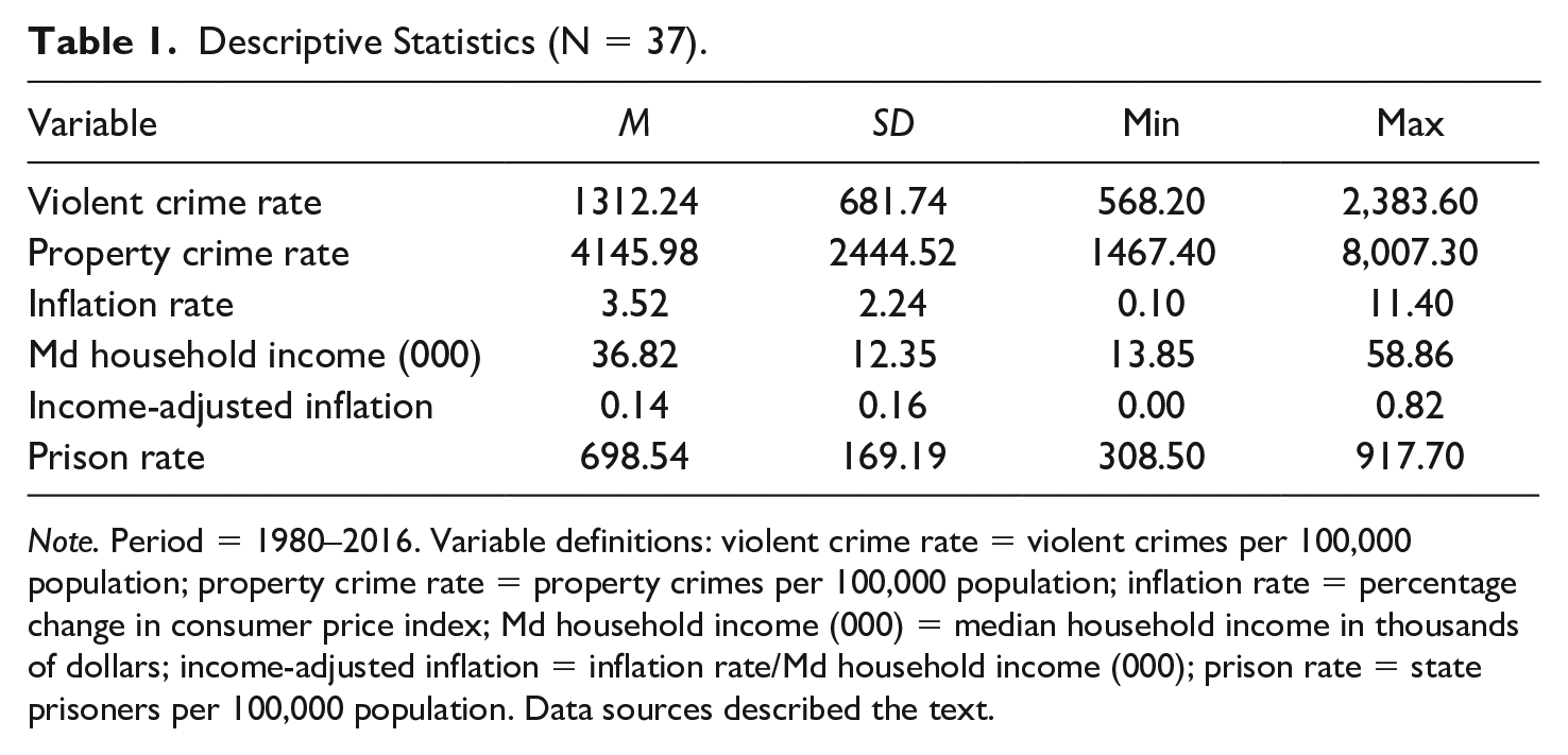
Note. Period = 1980–2016. Variable definitions: violent crime rate = violent crimes per 100,000 population; property crime rate = property crimes per 100,000 population; inflation rate = percentage change in consumer price index; Md household income (000) = median household income in thousands of dollars; income-adjusted inflation = inflation rate/Md household income (000); prison rate = state prisoners per 100,000 population. Data sources described the text.

New York’s violent and property crime rates between 1980 and 2016 are displayed in Figure 1. To eliminate scale differences and reveal the relationship between the trends in the two crime types, they are scaled on separate axes, with violent crime on the lefthand axis and property crime on the righthand axis of the figure. Both violent and property crime rates fell during the early 1980s and rose during the next few years, before falling continuously well into the current century during what has been termed the “Great American Crime Decline” (Zimring, 2007). What is also striking about the violent and property crime time trends is how closely they correspond (the Pearson’s correlation [r] between the two series is .98). This high degree of convergence suggests that the same sources of change over time in New York’s violent crime rate also underlie the change in the property crime rate.

Figure 1.

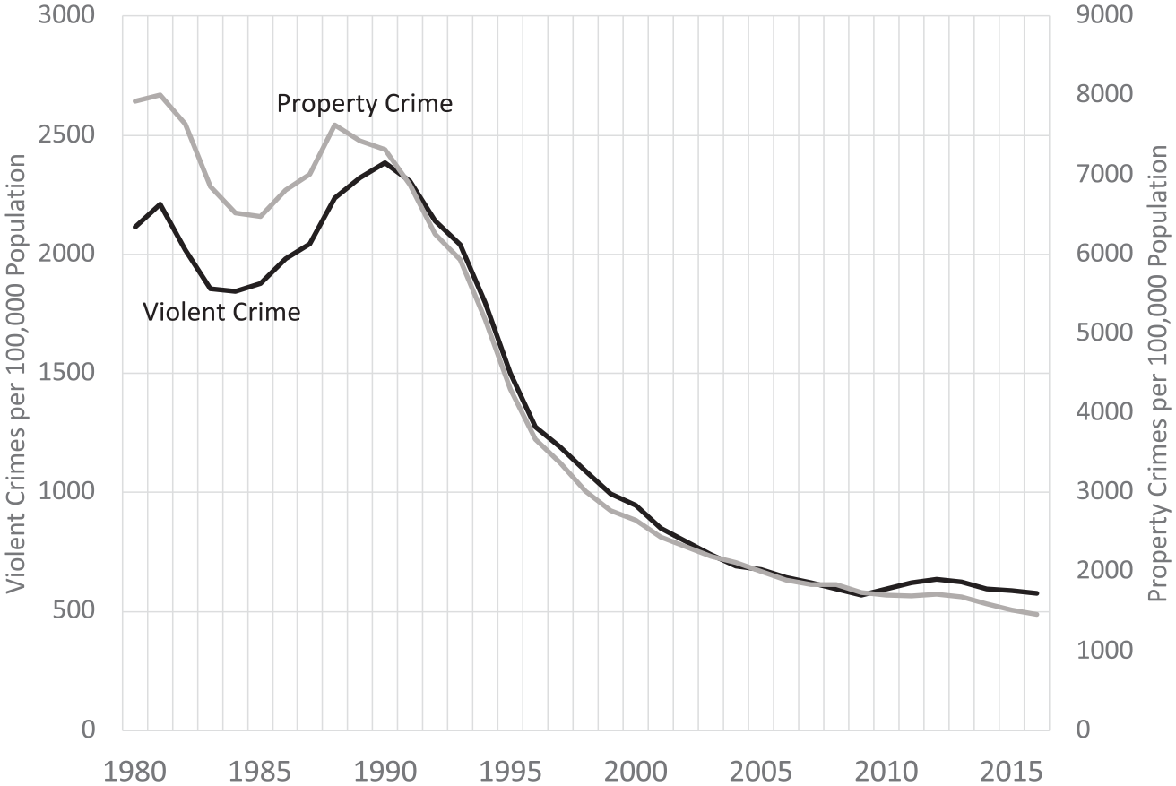
New York Violent and Property Crime Rates, 1980–2016.

Stationary Tests and First Differencing

A cursory glance at Figure 1 indicates that New York’s violent and property crime rates between 1980 and 2016 are nonstationary. Neither series exhibits a constant mean over time. This perception is confirmed by formal tests to determine whether the two time series contain a unit root. Both the augmented Dickey–Fuller (ADF) test and the Phillips–Perron (PP) test failed to reject the null hypothesis of a unit root for both series.⁶ New York’s violent and property crime rates between 1980 and 2016 are nonstationary and conform to a random walk.

We therefore converted the two series to first-differences and performed the same tests. The PP test rejected the null hypothesis that the first-differenced violent and property crime series contain a unit root at the conventional 5% level of significance (p = .03 for both series). Inspection of the first-differenced series indicates that the two series “drift,” meaning that the average first differences are not constant over time. When a drift term is added to the ADF model, the model rejects the null hypothesis of a random walk with drift at the 1% level of significance for both the violent crime and property crime first-differenced series. When converted to first differences, both series are stationary.

Forecasting Results

ARIMA forecast models were fit to the first-differenced violent and property crime rates between 1980 and 2016. We “held back” the years 2017 to 2021 from the models so they could be used to validate the forecasts from the 1980–2016 baseline period. The closer the forecasted first-differenced crime rates are to the observed rates during the validation period, the greater our confidence in the forecasts for 2022 to 2024 when the observed crime rates are unknown.

The forecasting results are presented in Figures 2 and 3. The figures display the observed and forecasted values of the crime series from 2000 to 2024. The solid line denotes the observed values from 2000 to 2021. The dashed line denotes the forecasts for 2000 to 2016, the dotted line indicates the forecasts for 2017 to 2021, the validation period, and the gray-shaded dotted line represents the forecasts for 2022 to 2024. In 2017, the first year of the forecast validation period, the New York’s observed violent crime rate dropped by 37 violent crimes per 100,000 population, while the forecasted rate shows little change. The changes in the observed and forecasted violent crime rates are fairly close during the next few years until 2021, when the observed rate increased by more than 80 violent crimes per 100,000, and the forecasted rate drops by about 25 violent crimes per 100,000. The forecasts indicate that New York’s violent crime rate should rise in 2022 and 2023. The rate in 2024 should exhibit little change over the previous year.

Figure 2.

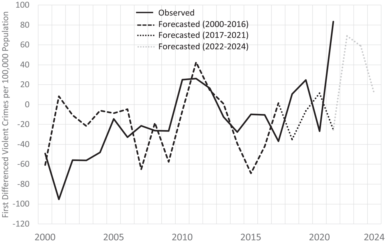
Observed and Forecasted Year-Over-Year Change in New York Violent Crime Rate, 2000–2024.

Figure 3.

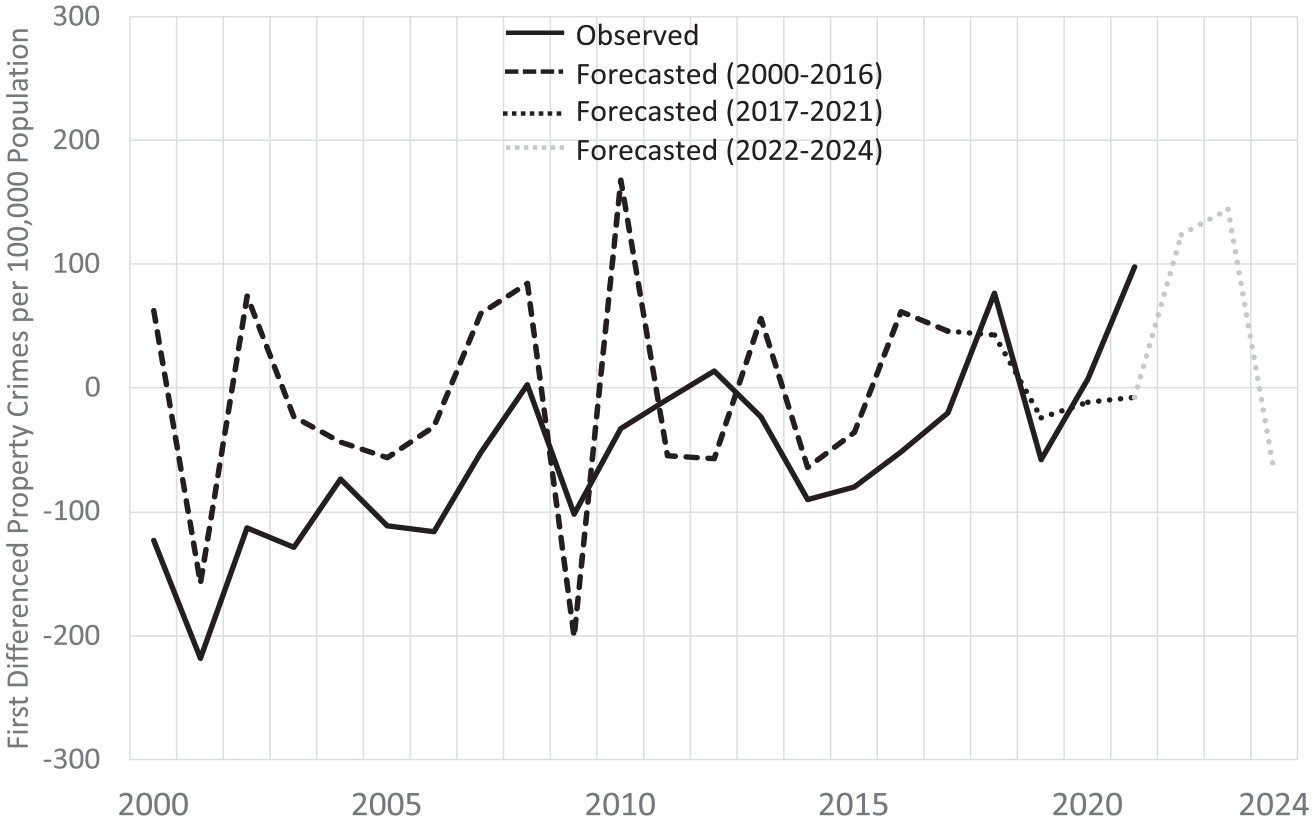
Observed and Forecasted Year-Over-Year Change New York Property Crime Rate, 2000–2024.

As shown in Figure 3, New York’s observed and forecasted first-differenced property crime rates are very similar between 2017 and 2021. In 2017, they diverge by just 66 property crimes per 100,000, by 34 in 2018 and 2019, and by just three in 2020. As with violent crime, the difference between the changes in the observed and forecasted property crime rates is larger in 2021, when the observed rate grew by nearly 100 property crimes per 100,000, and the forecasted rate falls slightly. The forecasts suggest that New York’s property crime rate should rise in 2022 and 2023 before falling in 2024.

In Table 2, the year-to-year forecasted changes in New York’s violent and property crime rate are added to the previous year’s rates to generate forecasts of the current year’s rates during the validation period. The best-fitting forecast model for violent crime is an ARIMA_(2,0,2) model, which contains two autoregressive terms and a first- and second-order moving-average term. The model forecasts a violent crime rate in 2017 of about 577 violent crimes per 100,000 population, which is about 7% above the observed rate of 538. The forecasted rates fall below the observed rates by about 8% and 5% in 2018 and 2019 and 7% above the observed rate in 2020. In 2021, the forecasted violent crime rate of 521 violent crimes per 100,000 is about 17% below the observed rate of 630. The mean absolute percentage error (MAPE) during the 5-year validation period indicates that, on average, the forecasted violent crime rate diverges in either direction from the observed rate by about 9%.

Table 2.

Forecasts of New York Violent and Property Crime Rates, 2017–2024.

	Violent crime (ARIMA_[2,0,2])			Property crime (ARIMA_[0,2,0])
	Observed rate	Forecasted rate	Percentage error	Observed rate	Forecasted rate	Percentage error
2017	538.5	576.9	7.13	1,447.5	1,513.6	4.57
2018	549.0	503.4	−8.32	1,524.6	1,490.3	−2.25
2019	573.6	542.8	−5.38	1,467.0	1,500.3	2.27
2020	546.7	585.0	7.00	1,474.5	1,455.8	−1.27
2021	630.2	521.4	−17.26	1,572.4	1,467.0	−6.71
MAPE			9.02			3.41
Mean	567.6	545.9	−3.82	1,497.2	1,485.4	−0.79
2022		699.1			1,696.0
2023		757.9			1,840.4
2024		768.2			1,774.5

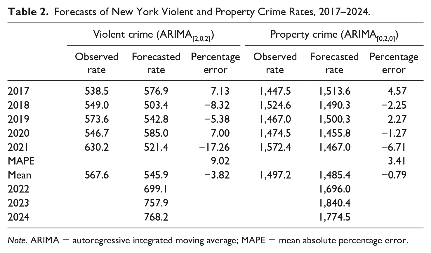
Note. ARIMA = autoregressive integrated moving average; MAPE = mean absolute percentage error.

The best-fitting forecast model for property crime is an ARIMA_(0,2,0) model. None of the forecasted property crime rates diverges from the observed rates by more than 7% during the validation period, and the average divergence is just 3.4%. The subsequent forecasts indicate a sizable rise in New York’s property crime rate in 2022 and a smaller rise in 2023, before falling in 2024.

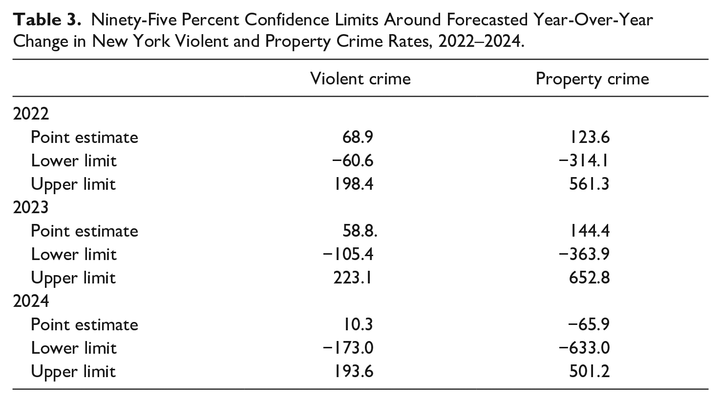
Contrary to Land and McCall’s (2001) advice, this exercise yields point forecasts of New York’s crime rates and not the kind of forecast cones they prefer. Nonetheless, it is important to create boundaries around the point forecasts to evaluate their utility for both policymaking and hypothesis testing. One approach is to use the confidence intervals around the estimates to define the forecast cones. The 95% confidence limits around the forecasted violent and property crime changes for 2023 and 2024 are very wide, as shown in Table 3. For example, the point forecast for the first-differenced property crime rate in 2022 is an increase of 124 property crimes per 100,000 population (see Figure 3). The upper limit of this forecast is 561 and the lower limit is −314. The comparable values for violent crime are 69, −61, and 198. These limits are much too broad to inform policy or theory. The conventional 95% confidence limits are arbitrary, but are a reminder of the statistical uncertainty of point forecasts and of the need to increase sample size or respecify forecast models, as needed, to improve forecast precision.

Table 3.

Ninety-Five Percent Confidence Limits Around Forecasted Year-Over-Year Change in New York Violent and Property Crime Rates, 2022–2024.

	Violent crime	Property crime
2022
Point estimate	68.9	123.6
Lower limit	−60.6	−314.1
Upper limit	198.4	561.3
2023
Point estimate	58.8.	144.4
Lower limit	−105.4	−363.9
Upper limit	223.1	652.8
2024
Point estimate	10.3	−65.9
Lower limit	−173.0	−633.0
Upper limit	193.6	501.2

If the analyst chooses to rely on the point forecasts as the best estimate of future crime rates, and the confidence intervals are very broad, some other method must be used to establish meaningful boundaries around the estimates. This usually means that the policymaker or researcher will have to decide how much forecast error is tolerable, which is a substantive and not a statistical decision. We will assume for current purposes that forecasted crime rates that diverge from the observed rates by no more than 10% are sufficiently accurate and precise for both policy and theory evaluation. Forecasts that fall outside of these limits would be uninformative, although they do suggest that the forecast model probably needs to be revised.

As shown in Table 2, the forecast errors for violent crime fall outside the 10% limit in 2021 and are inside the limit for the other years of the validation period. These results suggest that the forecast model for violent crime should be revisited to determine the source of the forecast error in 2021. One likely candidate is the exogenous shock to crime rates from the COVID-19 pandemic. The quarantines, lockdowns, and other dislocations resulting from the pandemic altered violent crime rates in ways no forecast model could have predicted. A conservative approach would be to rely on the 5-year mean forecasts instead of the yearly estimates for forecasting purposes. This would reduce the average forecasting error during the validation period, but it would not capture the forecasted rise in violent crime rates from 2022 to 2024. We conclude that the forecasting results for violent crime are acceptably precise on average and that the large error during 2021 was unavoidable.⁷

The story for property crime is somewhat different. The forecasted property crime rates during the validation period are well within the 10% tolerance limits. These limits were arbitrarily drawn, but even if the 10% divergence threshold were cut in half, the forecasted property crime rates would have been accurate and precise enough for both policy and research purposes between 2017 and 2020 and nearly so in 2021.

In our view, the forecasting results for New York’s violent and property crime rates inspire guarded optimism about the prospects for forecasting in criminology. The forecasted property crime rates are very close to the observed rates during the validation period and provide a reliable basis for forecasting property crime rates 3 years ahead. The same is generally true for the violent crime results. The forecast error for violent crime in 2021, however, is outside the 10% tolerance limits we placed around the estimates. More permissive limits could have been chosen, of course, but the optimal standard—how much error is acceptable—is not a statistical question but a matter of judgment and the preferred tradeoff between forecast accuracy and precision. The forecast error is also an important reminder of the challenge of unanticipated shocks to forecasting crime rates, or anything else. In addition, the wide confidence intervals around the forecast estimates diminish statistical confidence in the precision of the estimates. Some social scientists and statisticians argue that the emphasis on statistical significance is misguided, a position that also has attracted criticism (Mayo & Hand, 2022). We do not take a stance on this issue. But as long as significance tests remain widespread in scientific practice, improving the statistical precision of crime forecasts will remain an important task in the development of reliable forecasting methods and models in criminology.

Conclusion

Forecasting future crime rates, when done carefully on the basis of a credible forecasting model, is a natural and needed extension of the study of crime trends. Forecasting provides data to test theory that were not in the sample of observations used to develop the theory. Forecasting answers the perennial plea of policymakers, the press, and the public: You’ve told me what happened yesterday; now tell me what will happen tomorrow. The answers will not always be accurate or precise, but they will come from an explicable set of methods and decisions that assume that the probable future of crime rates is related to their past behavior and to the conditions known to influence it.

Modesty is the best policy when forecasting crime rates. Forecasts will almost always be off the mark in the presence of exogenous shocks that sever the future from the past and that no forecasting model could have predicted. A recent example is the COVID-19 pandemic, which affected crime rates in complex ways (Lopez & Rosenfeld, 2021). Another is the abrupt increase in inflation beginning in 2021 (Banerjee et al., 2023). Forecasts will also be incorrect when the conditions known to influence the crime rate change in unexpected ways. That is why forecasts should always be tested against out-of-sample conditions that are known, the approach taken here, before taking on the unknowable future. A useful way of presenting the forecasts is in the form of conditional probabilities: If these conditions hold, then the crime rate will be X. When uncertainty exists regarding the future state of crime-generating conditions, as it usually does, a range of probabilities can be estimated. For example, all else equal, if the inflation rate is 3%, then the crime rate will be Y. If the inflation rate increases to 5% or 7%, the crime rate will be Z. These conditional probabilities can then be used to construct forecast cones around the point forecasts. Finally, the strength of the association between exogenous conditions and crime rates may change over repeated observations, as when the impact of imprisonment on crime rates diminishes with increasing levels of imprisonment over time.

The forecasting exercise we have conducted is intended to revive interest in crime forecasting in criminology. We have tried to be explicit about the reasoning behind each of the steps taken to (a) ready the data for reliable forecasting, (b) specify an explanatory model to be used in multivariate forecasting, (c) choose a forecasting model, and (d) interpret the results. Each of these decisions is open to criticism and alternative approaches. While we believe the data, methods, and models used here are useful for stimulating discussion and analysis of crime forecasting, they can be augmented in several ways such as by increasing sample size and incorporating additional covariates to reduce sampling error.⁸ In addition, other types of forecasting models (e.g., exponential smoothing models, which give greater weight to more recent observations) should be applied to the study of crime trends and their performance should be assessed against the ARIMA methods used here.

Crime forecasting has fallen on hard times in criminology, but past mistakes should not prevent renewed attention to this important endeavor. There is much work to do, and this study has barely scratched the surface of the rich forecasting literature in other fields.⁹ Enough is now known about the behavior of crime rates to support short-run forecasts of the future. And testing our theories against future crime rates is the best way to improve our explanations of the past.

Footnotes

Declaration of Conflicting Interests

The author(s) declared no potential conflicts of interest with respect to the research, authorship, and/or publication of this article.

Funding

The author(s) received no financial support for the research, authorship, and/or publication of this article.

Notes

Author Biographies

Richard Rosenfeld is the Curators’ distinguished professor emeritus of criminology and criminal justice at the University of Missouri-St. Louis. He is a fellow and former president of the American Society of Criminology. His research focuses on crime trends and crime control policy.

Mark Berg is professor of sociology and criminology at the University of Iowa where he is also the interim director of the Public Policy Center. His recent research examined the situational determinants of interpersonal violence, violent crime trends, and the social determinants of physical health outcomes.

References

Banerjee

Hall

S. G.

Kouretas

G. P.

Tavlas

G. S.

(2023). Advances in forecasting: An introduction in light of the debate on inflation forecasting. Journal of Forecasting, 42, 455–463.

Box

G. E. P.

Jenkins

G. M.

Reinsel

G. C.

Ljung

G. M.

(2016). Time series analysis: Forecasting and control (5th ed.). Wiley.

Brockwell

P. J.

Davis

R. A.

(2016). Introduction to time series and forecasting (3rd ed.). Springer.

Cohen

L. E.

Felson

Land

K. C.

(1980). Property crime rates in the United States: A macro macrodynamic analysis, 1947-1977–with ex ante forecasts for the mid-1980s. American Journal of Sociology, 86, 90–118.

Cohen

L. E.

Land

K. C.

(1987). Age structure and crime: Symmetry versus asymmetry and the projection of crime rates through the 1990s. American Sociological Review, 52, 170–183.

DiIullio

(1995, November 27). The coming of the super-predator. Weekly Standard. https://www.washingtonexaminer.com/weekly-standard/the-coming-of-the-super-predators

Fox

J. A.

(1978). Forecasting crime data: An econometric analysis. Lexington Books.

Fox

J. A.

Piquero

A. R.

(2003). Deadly demographics: Population characteristics and forecasting homicide trends. Crime & Delinquency, 49, 339–359.

Gorr

Olligschlaeger

Thompson

(2003). Short-term forecasting of crime. International Journal of Forecasting, 19, 579–594.

10.

Haberman

(2014, April 6). When youth violence spurred “superpredator” fear. The New York Times. https://www.nytimes.com/2014/04/07/us/politics/killing-on-bus-recalls-superpredator-threat-of-90s.html

11.

Hyndman

R. J.

Athanasopoulos

(2018). Forecasting: Principles and practice (2nd ed.). OTexts.

12.

Land

K. C.

McCall

P. L.

(2001). The indeterminacy of forecasts of crime rates and juvenile offenses. Appendix B in Institute of Medicine, Juvenile Crime, Juvenile Justice. National Academies Press.

13.

Lau

(2020). Predictive policing explained. Brennan Center for Justice. https://www.brennancenter.org/our-work/research-reports/predictive-policing-explained

14.

Levitt

S. D.

(1996). The effect of prison population size on crime rates: Evidence from prison overcrowding legislation. Quarterly Journal of Economics, 111, 319–352.

15.

Lopez

Rosenfeld

(2021). Crime, quarantine, and the U.S. coronavirus pandemic. Criminology & Public Policy, 20, 401–422.

16.

Mayo

D. G.

Hand

(2022). Statistical significance and its critics: Practicing damaging science, or damaging scientific practice? Synthese, 200, Article 220. https://doi.org/10.1007/s11229-022-03692-0

17.

Rosenfeld

Levin

(2016). Acquisitive crime and inflation in the United States: 1960 - 2012. Journal of Quantitative Criminology, 32, 427–447.

18.

Schuster

(1995, February 17). “Bloodbath” predicted as children age. United Press International. https://www.upi.com/Archives/1995/02/17/Bloodbath-predicted-as-children-age/7792792997200/

19.

Steffensmeier

D. J.

Harer

M. D.

(1987). Is the crime rate really falling? An “aging” U.S. population and its impact on the nation’s crime rate, 1980–84. Journal of Research in Crime and Delinquency, 24, 23–48.

20.

Waters

(1996). Daniel Bell. Routledge.

21.

Zimring

F. E.

(2007). The Great American crime decline. Oxford University Press.

Forecasting Future Crime Rates

Abstract

Keywords

Background

Data and Methods

Results

Stationary Tests and First Differencing

Forecasting Results

Conclusion

Footnotes

Declaration of Conflicting Interests

Funding

Notes

Author Biographies

References