
Abstract
This study investigates the energy harvesting prospects of self-sustained flow oscillations emanating from grazing flow over a rectangular cavity by employing experimental and computational methods. Two cavity geometries with length-to-depth ratios of 2 and 3, exposed to an incoming flow of 30 m/s, were selected for the purpose. The power spectral density of the baseline cavity flows showed the presence of high-amplitude peaks whose frequencies agreed to those estimated from Rossiter’s feedback model. For energy harvesting, a piezoelectric beam was placed perpendicular to the aft wall and its natural frequency tuned to match closely with the dominant frequencies of the cavity flow oscillations. From the experiments, an average and maximum instantaneous power of 21.11 and 284.18 µW was recorded for the cavity with L/D = 2 whereas for the cavity with L/D = 3 the corresponding values were 32.16 and 403.46 µW respectively. Time-frequency analysis showed the forcing of the beam at the cavity oscillation frequency and the substantial increase in the amplitude of beam vibrations when this frequency was close to the natural frequency of the beam.
1. Introduction
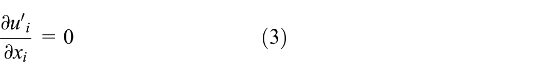
The quest to harness energy from surrounding natural resources can be dated back centuries. However, in the recent decade, with the advent of micro and nanoscale electronic sensors and systems, the scope has now expanded to conform to these scales as well. Finding power sources at these scales, especially cost-free, from the ambience where energy can be scavenged and harvested, have gained traction. The field has been made all the more conducive and pertinent owing to the flourish of technologies such as the Internet of Things (IoT), wireless sensor networks, MEMS-based portable devices and monitoring systems. Powering such microelectronic systems using a renewable source of energy would be a win-win situation for both society as well as the environment. They reduce wastage, maintenance cost and pollution of the environment.
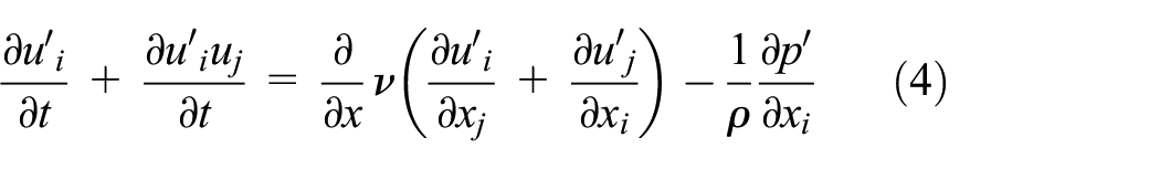
Pertinent to micro-scale power plants, recent research indicates that energy harvesting from fluid flows is a promising technique with broad applications (Hamlehdar et al., 2019). While conventional methods like turbines are suitable for large scale power generation, they are vastly inefficient, complicated and expensive at small scales (Mitcheson et al., 2008). The influence of damping forces and coil turns achievable at the MEMS scale makes turbines and other electromagnetic harvesters largely impractical in these applications. The harnessing methods employed to extract energy from fluid flow at these scales are largely vibrations-based, wherein energy from the flow is converted into mechanical vibrations of a transducer which further transforms them into electrical energy. Some of the most widely used transducers in research are based on electromagnetic and piezoelectric principles. Piezoelectric harvesters are particularly well-suited due to their scalability to miniature applications, low-voltage operation and easier tunability to high frequencies for resonant operations. Energy harvesting oscillators using this principle capture the structural vibrations caused as a result of flow-structure interaction or use the unsteady flow field created owing to a body placed in the flow. Energy harvesting from flutter and galloping belong to the former method while Vortex-Induced Vibrations belong to the latter.
In flutter-based energy harvesting, the vibration of energy harvesters is caused due to aeroelastic instabilities caused in a body due to the incoming airflow. The flow excites two or more modes of vibration in the body (typically a wing) that gets coupled and extract energy from the incoming flow. However, the airflow velocity has to attain a certain threshold value to activate the self-excited vibrations. Below the threshold value, the vibrations are damped by the wing material. When the flow velocity is increased far above the threshold value, large limit cycle oscillations occur due to aerodynamic and elastic non-linearities (Abdelkefi, 2016). Bryant and Garcia (2011) used a linear analytical model to study the onset of flutter vibrations and to study the frequency and wind speed when they start occurring. At higher wind speeds, they used a semi-empirical non-linear model to simulate the limit cycle oscillations using empirical coefficients from wind tunnel testing. Dunnmon et al. (2011) proposed a theoretical non-linear model for the self-excited limit cycle oscillations for an aeroelastic energy harvester. Concurrent experimental results on a NACA0015 airfoil of 550 mm span and 101 mm chord length produced a root mean square power of 2.5 mW at a wind velocity of 27 m/s. Using the apparatus, they were able to access a fifth of the flow energy for harvesting purpose.
In the galloping method, a bluff body like a prism is placed in a flow to excite aeroelastic instabilities above a cut-in velocity. The oscillations are of large amplitude and take place in a transverse direction to the flow. For galloping to occur, the aerodynamic lift coefficient derivative is required to be negative (Hartog, 1985). Sirohi and Mahadik (2011) conducted a successful attempt at harnessing energy using a cantilever beam with a piezoelectric patch attached to a triangular prism exposed transversely to the wind. They were able to harness a maximum power of 53 mW from the galloping motions of the structure at a wind velocity of 11.6 mph. They also supplemented their results with a detailed analytical model to deduce the voltage generated in their device across parameters like wind velocity, load resistance and beam geometry. Bibo et al. (2015) developed an aero-electromechanical model to describe the non-linear behaviour of an energy harvester that is under a combined galloping and base excitations.
Safety considerations become essential for flutter and galloping methods at higher wind speeds since the amplitude of oscillations can get inordinate. Another disadvantage with flutter and galloping is that they need sizeable structures to capture the energy which may make them difficult to adapt for internal flows. In Vortex-Induced Vibrations (VIV), the unsteady vortex shedding by a bluff body is used to induce a periodic fluid dynamic force on a structure, resulting in its oscillations. When coupled to an energy harvester, this oscillating motion of the structure is converted to electric energy. Wen et al. (2014) utilized a VIV based energy harvester using a cuboidal bluff body and a piezoelectric cantilever beam placed in the wake region. They recorded power of 1 µW at an airflow velocity of 2 m/s, corresponding to an eigen frequency of 5 Hz for the cantilever beam. Allen and Smits (2001) used a flat plate oriented normally to the incoming flow to move a flexible PVDF (polyvinylidene fluoride) cantilever in a water tunnel.
Apart from the above, there have also been studies aimed at harvesting energy from flow-induced acoustic resonance. Matova et al. (2011) used air oscillations in a Helmholtz resonator to vibrate a piezoelectric energy harvester. They tuned the frequency of the Helmholtz resonator to match with that of the piezoelectric diaphragm they used in the bottom of the resonator and were able to harvest 2 µW at an airflow velocity of 13 m/s. Zou et al. (2015) used a fluidic 1 mm diameter air jet to induce acoustic resonance inside a 10 mm long pipe resonator where a PZT-5H piezoelectric transducer was embedded. The harvester yielded a power of 85 mW relative to an airflow velocity of 159 m/s. Akaydin et al. (2010b) placed short PVDF piezoelectric cantilever beams in the wake region of a cylinder at Reynolds number range 10,000–21,000. When resonance occurred at Re = 14,800, maximum power of 4 µW was obtained when the beam was kept at a downstream distance twice the cylinder diameter (Akaydin et al. 2010a). Another exciting development happened with exploring turbulence-induced excitation (Akaydin et al., 2010a). Goushcha et al. (2015) explored the feasibility of energy harvesting from a turbulent boundary layer. They placed PVDF piezoelectric beams on turbulent boundary layers where
When it comes to harvesting energy from unsteady flow fields, the potential of cavity flow oscillations as a possible candidate is worth exploring. Research into cavity flows goes back as early as the 1950s. Grazing flow over certain rectangular cavity cut-outs is known to generate self-sustaining oscillations. Rossiter (1964) was one of the first investigators to propose a physical model that attributed to the generation of tones. According to his model, vortical disturbances shed from the cavity leading edge convect downstream and impinge at the aft wall. This impingement creates a transient high-pressure zone in front of the aft wall that generates an acoustic pressure wave that propagates in the upstream direction. This acoustic wave acts as feedback and further induces vortical disturbances at the cavity leading edge, which convects downstream to continue the cycle. While the vortical convection has been debated since they are not observed in all flow conditions, the presence of the acoustic feedback between the front and aft wall has been well established and is widely accepted. Heller and Bliss (1975) constructed an analytical model where they assumed the shear layer oscillations as flapping motions that periodically adds and removes mass into the cavity near the trailing edge, thus creating pressure fluctuation there. Cavity flow oscillations are largely undesirable, and several methods have been investigated to control them (Cattafesta et al., 2003; Saddington et al., 2016b; Thangamani and Kurian, 2013).
The various cavity flow control methods aim at disrupting one or more components of the feedback cycle that is responsible for the oscillations (Saddington et al., 2016a; Thangamani et al., 2014; Zhang et al., 1998). While detrimental otherwise, the self-sustained oscillations have the potential to power micropowered devices if harvested efficiently. There is a semi-empirical relation governing the frequency of oscillations, and this can be used to tune the harvester to lock in with the flow oscillations in order to derive maximum power. These concepts are explored in this work, through experiments and computations, and the potential of cavity flow oscillations for energy harvesting has been studied. The results show promise and justify further investigations. Possessing a simple geometry, a cavity flow-based energy harvesting device can be easily envisaged in numerous scenarios such as aircraft, automobiles, pipelines and even rivers for powering sensors.
In this work, a preliminary study to investigate the application of cavity flow oscillations for micro-energy harvesting is carried out. For this, a rectangular cavity of specific geometrical parameters that are expected to generate high-amplitude tones had been selected and tested for its unsteady pressure environment. A piezoelectric cantilever beam is fixed inside the cavity and tuned to lock in with the cavity oscillation frequencies and the power generated by the harvester is measured across a single resistor load. Due to the complex and transient nature of the flow, computer simulations were also carried out for one of the baseline cavity flow case to understand the flow features that give rise to the unsteadiness.
2. Experimental details
The experiments were carried out at the Thermofluids lab of the University of Southampton Malaysia. The chief aim behind the experimental design was to construct a small, simple apparatus that is capable of generating micro-wattage power by harnessing cavity-generated flow oscillations. For this, two small bespoke test sections, each embedded with a different rectangular cavity on one side of the wall was fabricated using transparent acrylic material (as shown in Figure 1). The test section was fitted to the air outlet of a small-scale wind tunnel manufactured by TecQuipment®, called as AF10. The AF10 can deliver a uniform airflow of velocity up to 30 m/s. The whole test section is 310 mm long and has an inlet of dimensions 100 mm × 50 mm. Air flow to the test section is regulated by a control valve before letting into a settling chamber. From the settling chamber, the air is accelerated through a convergent nozzle to a rectangular exit. Some minor components of the test section, like clamps and microphone fixtures, were 3D printed. The objectives of the experiments were to study the flow unsteadiness created due to the presence of the cavity, deduce the location and configuration to fit a piezoelectric beam inside the cavity and then measure the power generated by a piezoelectric energy harvester.
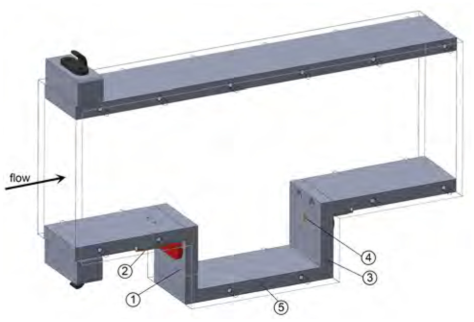
Test Section embedded with cavity. Numbered components show the (1) front wall, (2) front wall microphone, (3) aft wall, (4) aft wall microphone and (5) cavity floor.
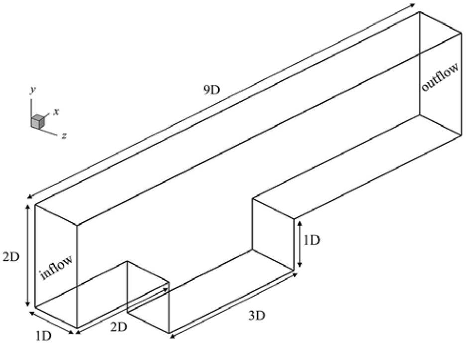
The unsteadiness created inside a cavity environment is largely dependent on the length-to-depth (L/D) ratio of the cavity (Tracy and Plentovich, 1993). Cavities with L/D < 10 are classified as open cavities whereas those with L/D > 10 as closed cavities. However, this demarcation is also dependent on the Mach number of the incoming flow. In open cavities, the shear layer separating from the leading edge of the cavity bridges across the cavity length without touching the cavity floor whereas in closed cavities the shear layer touches the floor. There is also a transitional phase (transitional cavities) between the two. Open cavities have been known to exhibit high-amplitude tones due to the presence of an effective feedback cycle. Oscillations are generally absent in closed cavities since the shear layer does not directly impinge on the aft wall to initiate the feedback cycle. Hence for the current studies, two rectangular cavity geometries were selected – the first with an L/D = 2 and the second with L/D = 3. Both the geometries clearly belong to the open cavity flow classification and can be expected to generate significant flow oscillations. For brevity, the test section embedded with the cavity of L/D = 2 will be referred to as CM2 (Cavity Model with L/D = 2) and one with L/D = 3 as CM3. The cavity dimensions for CM2 is L × W × D = 100 mm × 50 mm × 50 mm whereas of that of CM3 is 150 mm × 50 mm × 50 mm. The length-to-width (L/W) ratio affects the three-dimensionality and tonal amplitudes associated with the flow. The L/W ratio of CM2 and CM3 is 2 and 3, respectively. In his studies on the effect of cavity width, Ahuja and Mendoza (1995) found that the sound power levels of the cavity increased with an increase in cavity width, keeping other factors constant. However, the tonal frequencies remained unaffected with the change in cavity width. Hence, if other parameters are kept the same, an open cavity with a low value of L/W is desirable from an energy harvesting perspective.
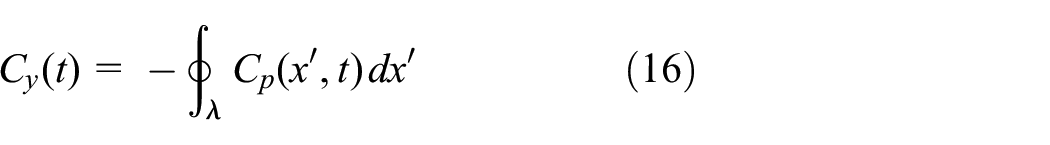
The origin for the flow coordinate system in this study is fixed at the midpoint of the cavity leading edge. The incoming flow direction is treated as the x-axis and the cavity span direction as the z-axis (Figure 6). The incoming flow speed for the experiments was set to 30 m/s, and the velocity was measured using a pitot tube and pressure tap located at the test section inlet. The boundary layer at the cavity leading edge was measured using a boundary layer probe mounted on a screw gauge and the thickness based on 99% freestream velocity,
For the current case, n = 5.8 was found to be the best fit for the boundary layer profile measured (Figure 2). Based on the estimated displacement thickness value, the blockage to the flow at the transverse plane at cavity leading edge, calculated as

Boundary layer profile measured at
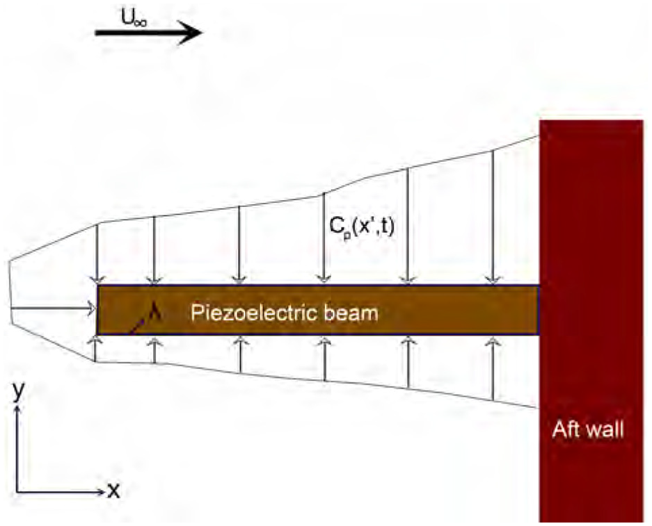
For energy harvesting, a single-layered piezoelectric beam bender, S128-H5FR-1107YB, commercially manufactured by Midé was used. The piezoceramic material used in the beam is PZT-5H sandwiched between copper electrodes and a packaging material FR4. The whole beam weighs 2 g and is suited for harnessing vibrations at high frequencies up to 660 Hz. The various properties of the piezoelectric material are given in Table 1. The beam measured 53 mm × 20.8 mm × 0.71 mm in size and was fixed at one end to be used as a vibrating cantilever. For energy harvesting, the beam was located perpendicular to the cavity wall, as shown in Figure 3. The reasoning and effect of placing the beam at the aft wall and front wall have been discussed in subsequent sections. The piezoelectric beam was mounted perpendicular to the aft wall through a narrow slit of 1.2 mm thickness. A clamp (shown in Figure 4), screwed on to a 3D printed fixture, was used to install and control the vibrating length of the piezoelectric beam.
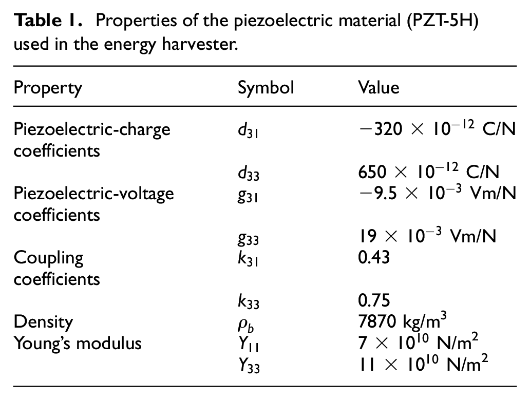
Properties of the piezoelectric material (PZT-5H) used in the energy harvester.
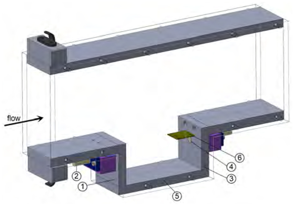
Test section with piezoelectric beam located at aft wall. Numbered components show the (1) front wall, (2) front wall microphone, (3) aft wall, (4) aft wall microphone, (5) cavity floor and (6) piezoelectric beam.
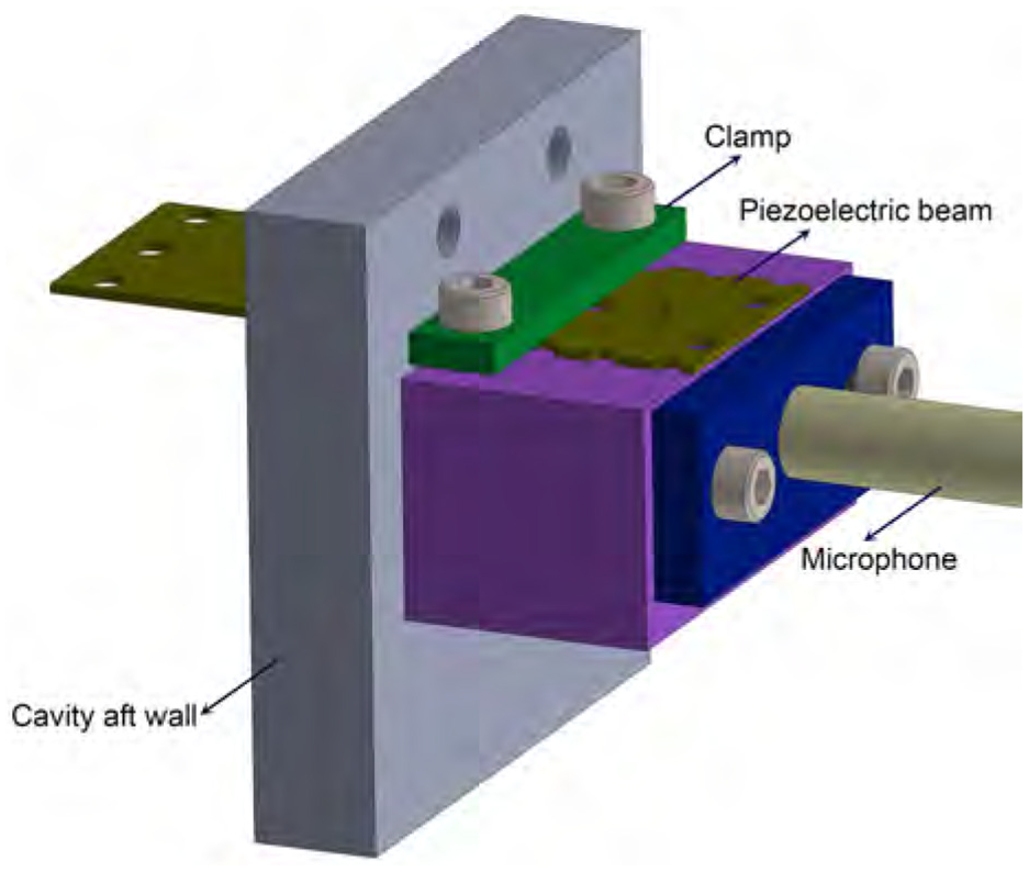
Detailed view of piezoelectric beam installed at aft wall.
The fluctuating pressure measurements were made using PCB manufactured 130F21 model pre-polarized microphones. The 130F21 model is an Integrated-Circuit Piezoelectric (ICP®) microphone that has a high sensitivity of 45 mV/Pa and is built with an integrated preamplifier. They have a diameter of 1/4″ and were flush-mounted on the cavity surface (Figure 5). Three such microphones were used for both the models CM2 and CM3. They were placed at locations (x/L, y/D, z/W) = (0, −0.42, 0), (0.5, −1, 0) and (1, −0.42, 0). This enables comparison of the fluctuating pressure levels at the front wall, cavity floor and aft wall, respectively. The signals obtained from the microphones and energy harvester were acquired and recorded using a National Instruments data acquisition module NI USB-4431. The NI USB-4431 has a 24-bit resolution and is capable of acquiring signals at a sampling rate of up to 102.4 kHz. It is specifically designed for sound and vibration measurements and thus well suited to the current study. The analog-to-digital conversion and signal conditioning are also carried out by the NI USB-4431, which was interfaced and controlled through LabVIEW software. For any given test, the signals from three microphones and the energy harvester, if present, were acquired simultaneously. The experiments were found to be repeatable, and the frequencies of the dominant mode of cavity oscillations were found to be invariable between different runs. To quantify Type A uncertainty (Kirkup and Frenkel, 2006) in the measurement of amplitude, ten different runs were carried out under the same test conditions, and the standard uncertainty based on n observations and a standard deviation

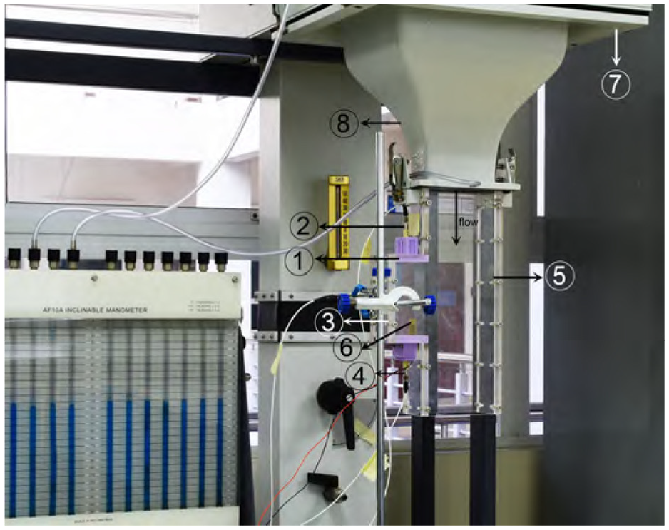
Test section assembly attached to flow bench (flow direction is vertically downwards). Numbered components show the (1) front wall, (2) front wall microphone, (3) cavity, (4) aft wall microphone, (5) rectangular test section with embedded cavity, (6) piezoelectric beam, (7) settling chamber and (8) converging nozzle.
The maximum standard uncertainty in amplitude seen in the power spectral density plots, calculated using equation (2), for any of the first three cavity modes of oscillation was ±0.71 Pa2/Hz.
3. Computational details
Numerical simulations were carried out to provide insights into the unsteady flow structures that develop in the cavity. The main motive was to understand the fluctuating environment inside the baseline cavity so as to use this information to arrive upon a rational location to place the piezoelectric beam inside the cavity. In order to achieve this, only the CM3 was simulated since it showed higher levels of unsteadiness during the experiments. The simulation was performed using ANSYS Fluent 19.1 based on the cell-centred finite volume discretization method. The incompressible large-eddy simulation (LES) technique was adopted in the present study to predict the pressure fluctuations inside the cavity region. The filtered mass and momentum transport equations are given by:

where
where
and

where
The filtered Navier-Stokes equations were solved using the pressure-based solver. The Semi-Implicit Method for Pressure-Linked Equations (SIMPLE) scheme was employed in the solver for pressure and velocity coupling. In order to reduce the effect of numerical diffusion in the simulation, the convective fluxes were discretized using second-order-accurate bounded central differencing scheme. The discretized transport equations were advanced in time by an iterative time-advancement scheme with twenty inner iterations. A time-step size of
The geometry of the computation domain is shown in Figure 6. The dimensions of the cavity are the same as the experimental model which has a length-to-depth ratio of 3, a width of 1D and a length of 0.15 m. For the rectangular channel above the cavity, the height and the width of the rectangular channel are equal to the experimental model. The inflow boundary is located 2D away from the upstream wall of the cavity whereas the outflow boundary is 4D away from the downstream wall of the cavity. The origin of the coordinate system is located at the centre of the leading edge of the cavity. The computational domain consists of 1.6 million cells (250 × 80 × 80) inside the cavity region and 3.36 million cells (350×120×80) inside the rectangular channel above the cavity. A total of 30 cells were clustered in a 0.1D space region near the walls of the rectangular channel with a stretching ratio of 1.02. The first cell is 0.0002D away from all the wall, corresponding to a
Geometry of the computational domain.
The inflow velocity profile was obtained from a separate Reynolds averaged Navier-Stokes (RANS) simulation of a rectangular channel with a cross-section area identical to the experimental model and a length of 4D. In this simulation, a uniform velocity profile with a relatively low turbulent intensity of 0.5% was assigned at the inlet. The freestream velocity was maintained the same as that of experiments. The velocity profile obtained from the RANS simulation was then applied at the inflow boundary of the cavity model. At the outflow boundary of the cavity model, a traction-free boundary condition was assigned. All the walls were treated as no-slip surfaces.
4. Grid resolution effects
Before comparing the numerical results with the experimental data, the effect of grid resolution of the computational model was examined. Two different computational models were generated to evaluate the influence of spanwise and streamwise grid resolutions. The first model consists of about 0.5 million cells (150 × 80 × 4 0) inside the cavity and 1.02 million cells (350 × 85 × 40) in the rectangular channel. The mesh is referred to as the coarse mesh. The second model consists of 1.6 million cells (250 × 80 × 80) inside the cavity and 3.36 million cells (350×120×80) in the rectangular channel and is referred to as the fine mesh. The computational grid on the symmetry plane and the cross-section of the fine mesh model is illustrated in Figure 7. For both models, the cell sizes at the near walls of the cavity and rectangular channel were kept the same as described in the previous section. The statistical data were collected with a physical sampling time of 0.6 s, after a relaxation time of 0.11 s (approximately seven flow-through times) which is long enough for the statistically steady solution to be reached.
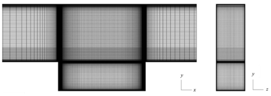
View of the grid distribution in the x–y plane (a) and the y–z plane (b) of the computation domain.
Figure 8 shows the profiles of the normalized mean streamwise velocity component,
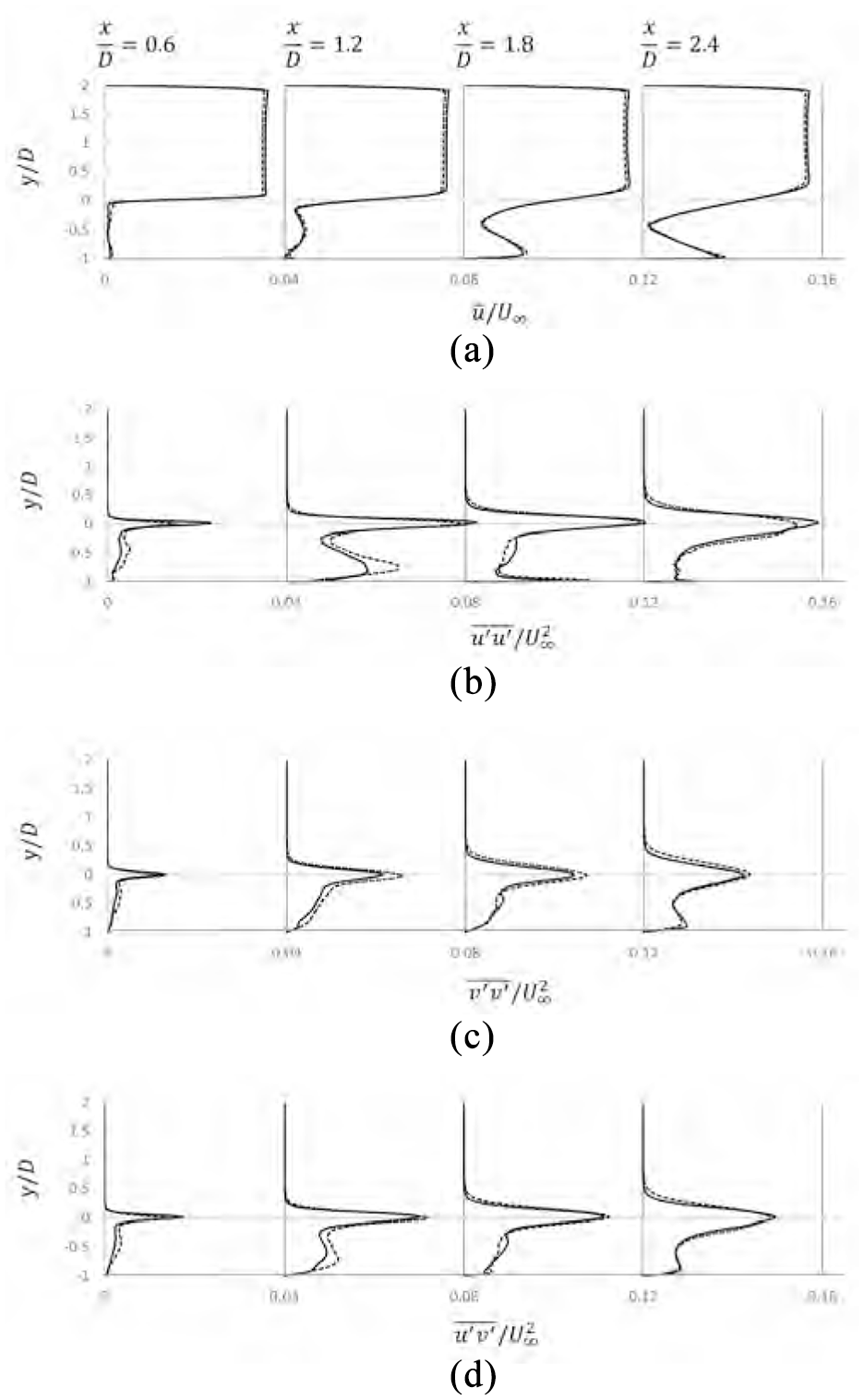
Comparison of the normalized mean streamwise velocity
5. Results and discussion
5.1. Baseline cases
To effectively harness the oscillatory energy of the flow, it is imperative to understand the nature of pressure unsteadiness and flow pattern generated in the cavity environment. Hence, the results of the clean cavity without any energy harvester, also known as the baseline cavity, are discussed first. The frequencies of flow oscillations were deducted experimentally from acoustic pressure data obtained using the microphones flush-mounted on the cavity front wall, floor and aft wall. The signals from the three microphones were acquired simultaneously at a sampling rate of 32,768 samples per second. For a given tunnel run, a total of 327,680 samples were collected over 10 s. The data obtained were used to plot the power spectral density using Welch’s method. To evaluate the spectrum, the 327,680 samples that were obtained per channel were segmented to 8192-point Fast Fourier Transforms (FFT) with a 50% overlap using a Hamming window, yielding a frequency resolution of 4 Hz. To get an accurate shape of the frequency spectrum for the cavity, spectral data from ten different tunnel runs were ensemble-averaged and the spectra thus obtained for CM2 and CM3 have been shown in Figures 9 and 10 respectively.
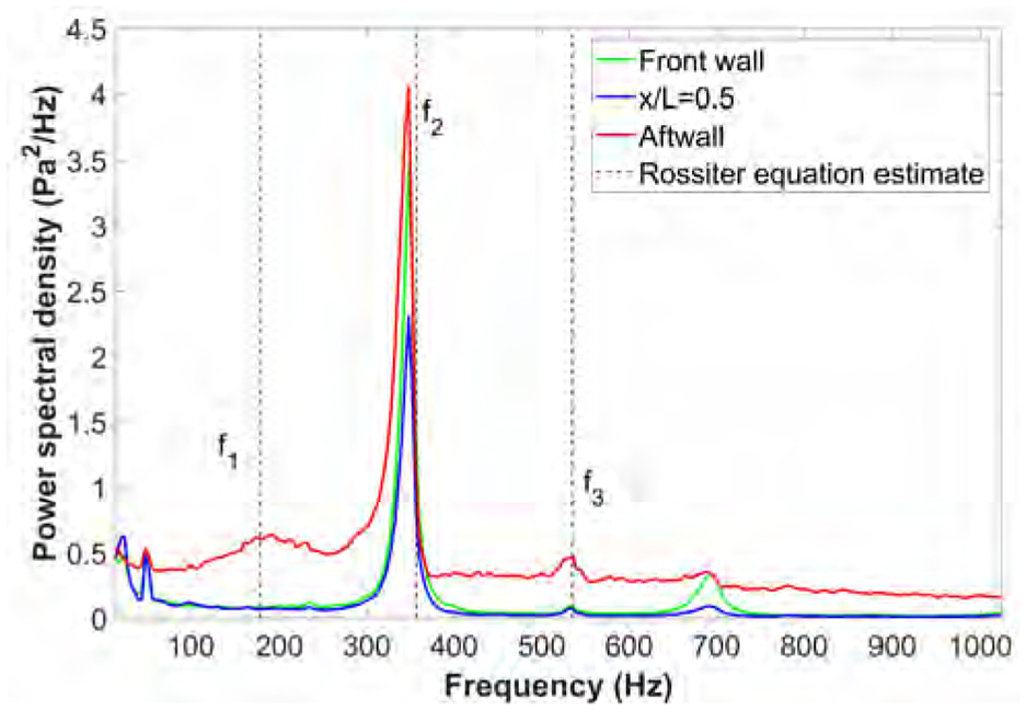
Baseline power spectral density for CM2 shown along with frequencies estimated using equation (9).
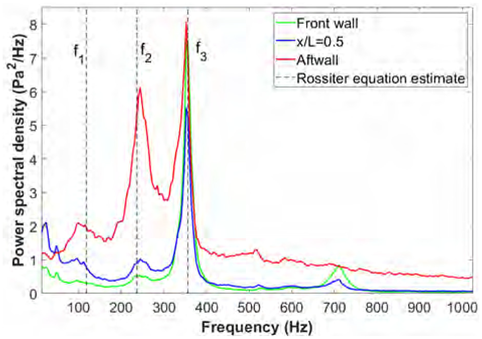
Baseline power spectral density for CM3 shown along with frequencies estimated using equation (9).
From the power spectral density plots of CM2 and CM3, high amplitude peaks can be discerned at specific frequencies. The first three modes of cavity flow oscillation will be hereafter denoted as
Rossiter used an empirical formula given by equation (9) to estimate the cavity frequencies by accounting for the various elements in his proposed model.
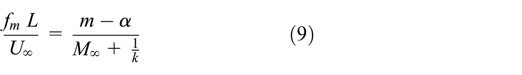
In the above equation,
5. 2 Computational results
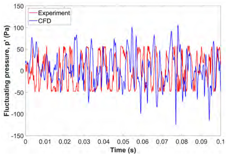
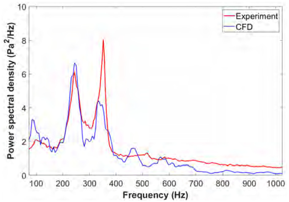
To decide upon the location and manner for placing the piezoelectric beam, an understanding of the flow field inside the cavity is essential. For this, computational simulation results have been utilized to visualize the flow. The fluctuating pressure data at corresponding locations were used to validate the computational results, and the agreement between experiments and CFD was found to be fair. Figures 11 and 12 show the comparison between the time series of fluctuating pressure,
Comparison of power spectral density at aft wall between measurement and CFD (CM3).
Comparison of fluctuating pressure at aft wall between measurement and CFD (CM3).
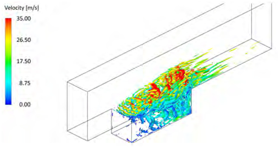
To extract the oscillatory energy of the flow, the piezoelectric beam has to be placed at a location where the pressure forces acting on it are high and periodic, subjecting it to vibrations with high tip-deflections. Figures 13 and 14 show the RMS contour plot of the fluctuating pressure and velocity respectively at the midplane. Contours of high fluctuations are concentrated towards the aft wall lip, making it an attractive position to place the beam. It was decided to locate the transducer perpendicularly to the aft wall at a distance of 0.22D down from the lip. This would utilize, without breaking up, the entire high fluctuating ‘red’ region shown in Figure 13.
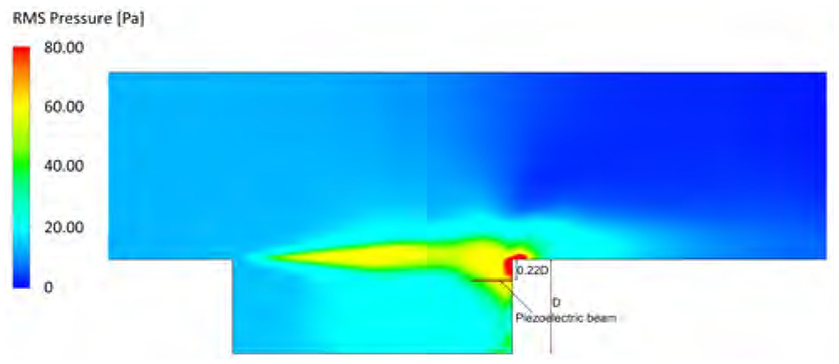
Aft wall location of the piezoelectric beam for CM3 superposed with RMS pressure contour.
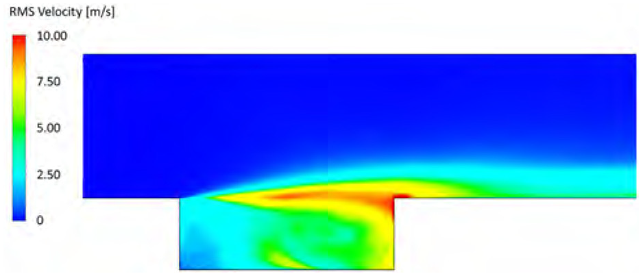
RMS velocity contour for CM3 at mid-plane.
While Figures 13 and 14 give the RMS quantities, from an instantaneous and temporal perspective, the free shear layer spanning the cavity is a dynamic region characterised by high vortical activity and the presence of coherent structures. The Q-criterion vortex identification method by Hunt et al. (1988) is used to educe the vortical structures that develop in the cavity. The regions of the vortex are defined by the second invariant of the velocity gradient tensor
Iso-surfaces of Q criterion.
5.3. Piezoelectric beam in cavity
To maximize the energy harvested by the piezoelectric beam, it would be judicious to tune the natural frequency of the piezoelectric beam to match closely and ‘lock-in’ with the cavity oscillation frequencies, in order to achieve high amplitudes. The tuned natural frequency of the piezoelectric beam is denoted as
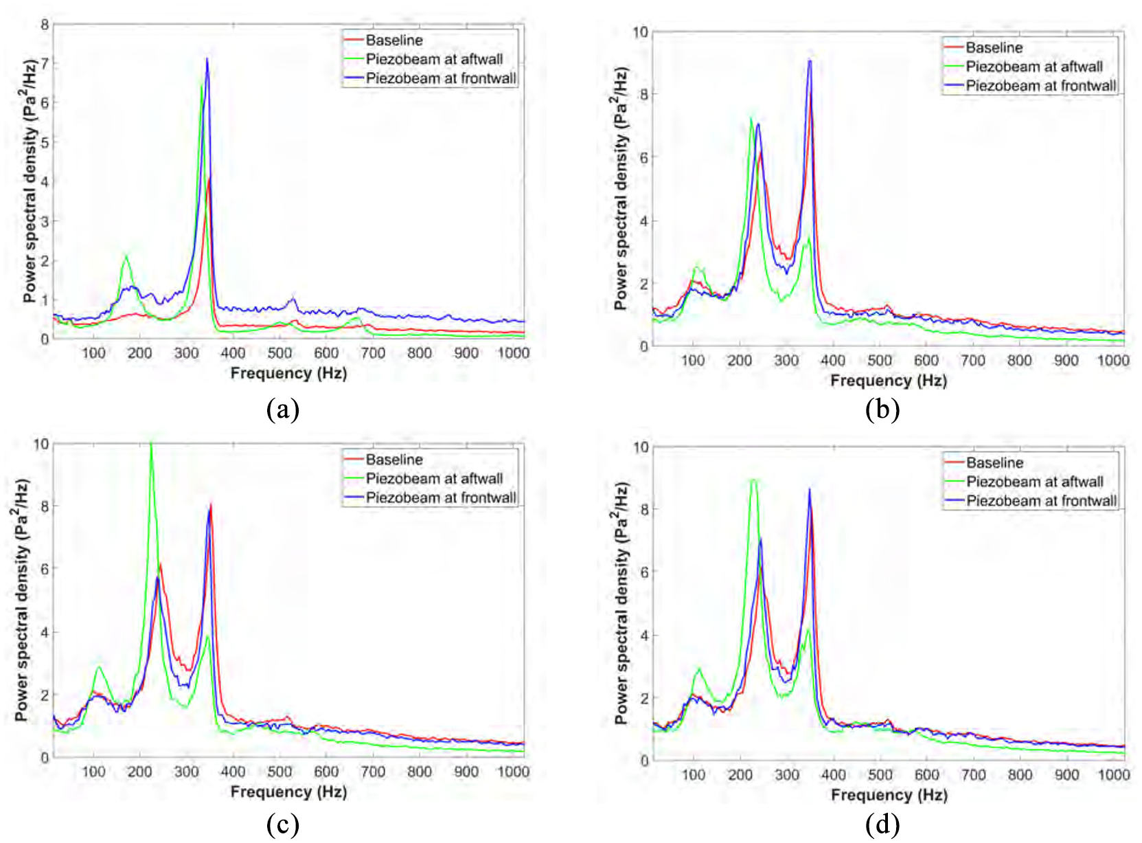
Effect of placing the piezoelectric beam on the cavity oscillation frequencies: (a)
For CM3, with the introduction of the piezoelectric beam at the aft wall, an appreciable change of 8.2% in frequency value was noticed for
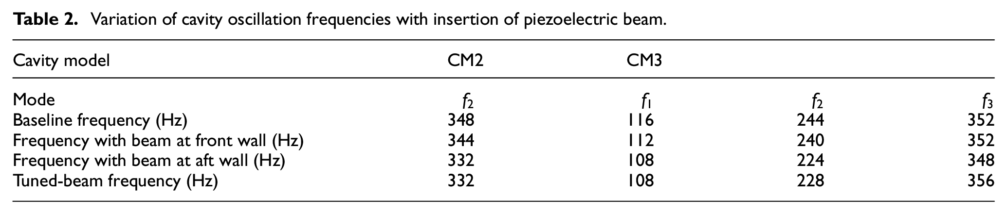
The change in the different mode frequencies against the tuning frequency of the piezoelectric beam has been tabulated in Table 2. Three beam natural frequencies (108 Hz, 228 Hz and 332 Hz) were tested for CM3 to match with
Variation of cavity oscillation frequencies with insertion of piezoelectric beam.
Changing the clamping location of the beam (refer Figure 4) alters the resonating length of the beam, thus varying its resonant frequency. The natural frequency of the beam,
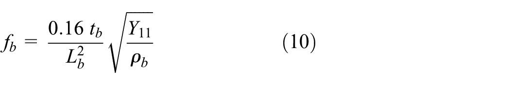
where
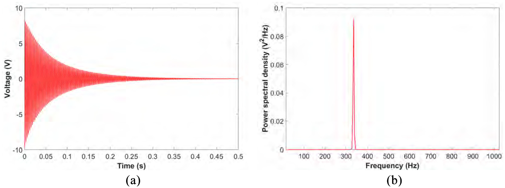
Voltage output and the corresponding power spectral density of a typical ring out test on the piezoelectric beam: (a) damping of the voltage signal when beam vibrates freely after release and (b) corresponding power spectral density showing the damped natural frequency.
Resonance of the beam will be achieved when
which implies that the tuning frequency is very sensitive to the clamping location. The
Variation of open circuit
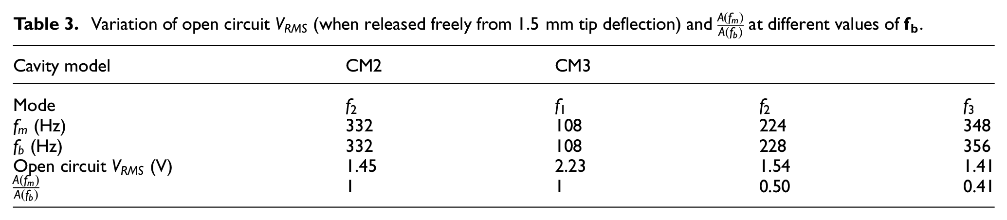
The values of
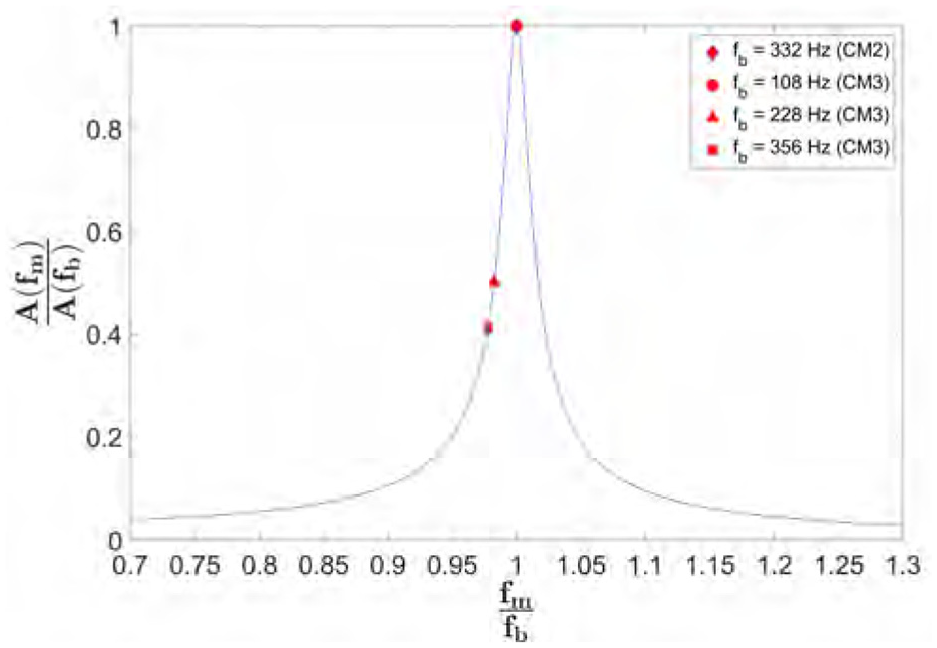
Effect of deviation of
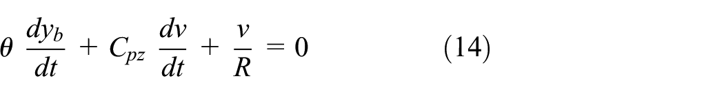
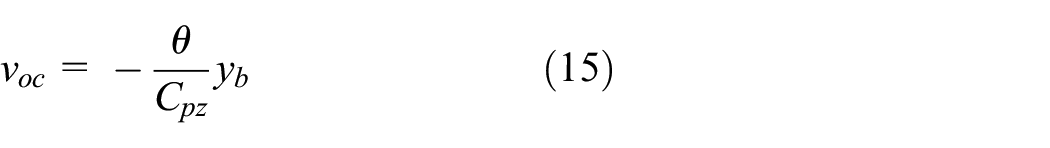
Assuming a single degree-of-freedom for vibrations, the piezoelectric beam under the influence of periodic forcing from the cavity flow field undergoes displacement that can be described (Zhao et al., 2013) by equations (13) and (14) as
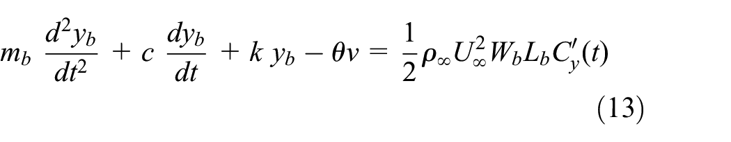
where
where
where
5.4. Power generation
The power harvested was estimated by measuring the voltage across the resistor load. The voltage signal across the resistor load was acquired at the same sampling speed as that of the microphone signal. From a given discrete voltage signal (
The comparison of power spectral densities between the microphone signals at the aft wall and the corresponding piezoelectric beam (located at aft wall) voltage signal during the energy harvesting tests, is shown in Figure 20. The amplitudes have been normalised by maximum value to juxtapose the two spectra for comparison.
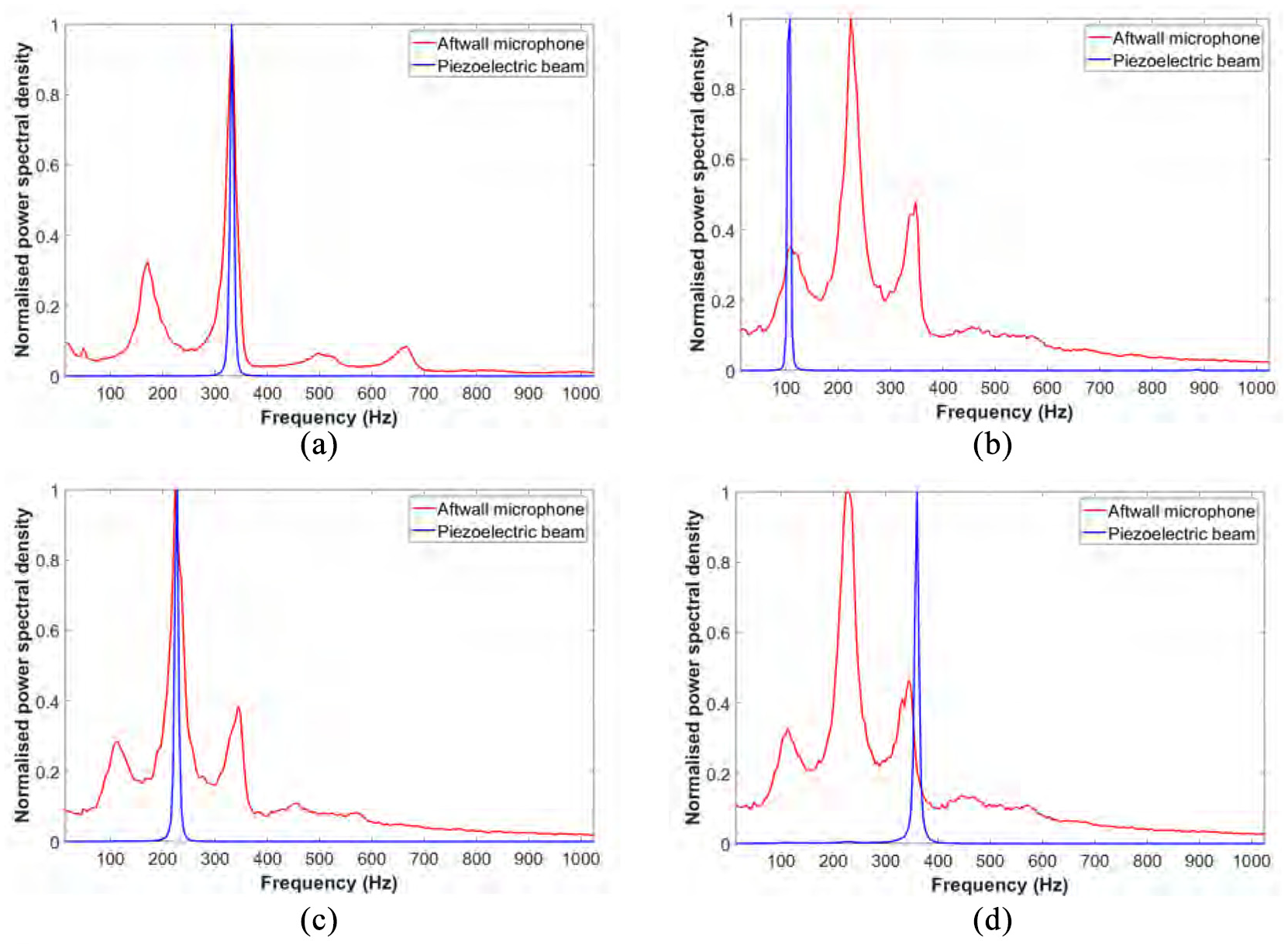
Comparison of normalised power spectra of aft wall microphone signal and piezoelectric beam located at aft wall: (a) lock in between beam and cavity mode
The instantaneous power generated was estimated by measuring the voltage across a load resistance abridging the piezoelectric beam terminals. Since the power generated varies with the load, a range of load resistance values were used to determine the optimal resistive load for a given piezoelectric beam setting. The average power variation for CM2 when the beam was tuned to 332 Hz natural frequency is shown in Figure 21(a). The maximum average power was recorded when the beam was located at the aft wall and was 21.1
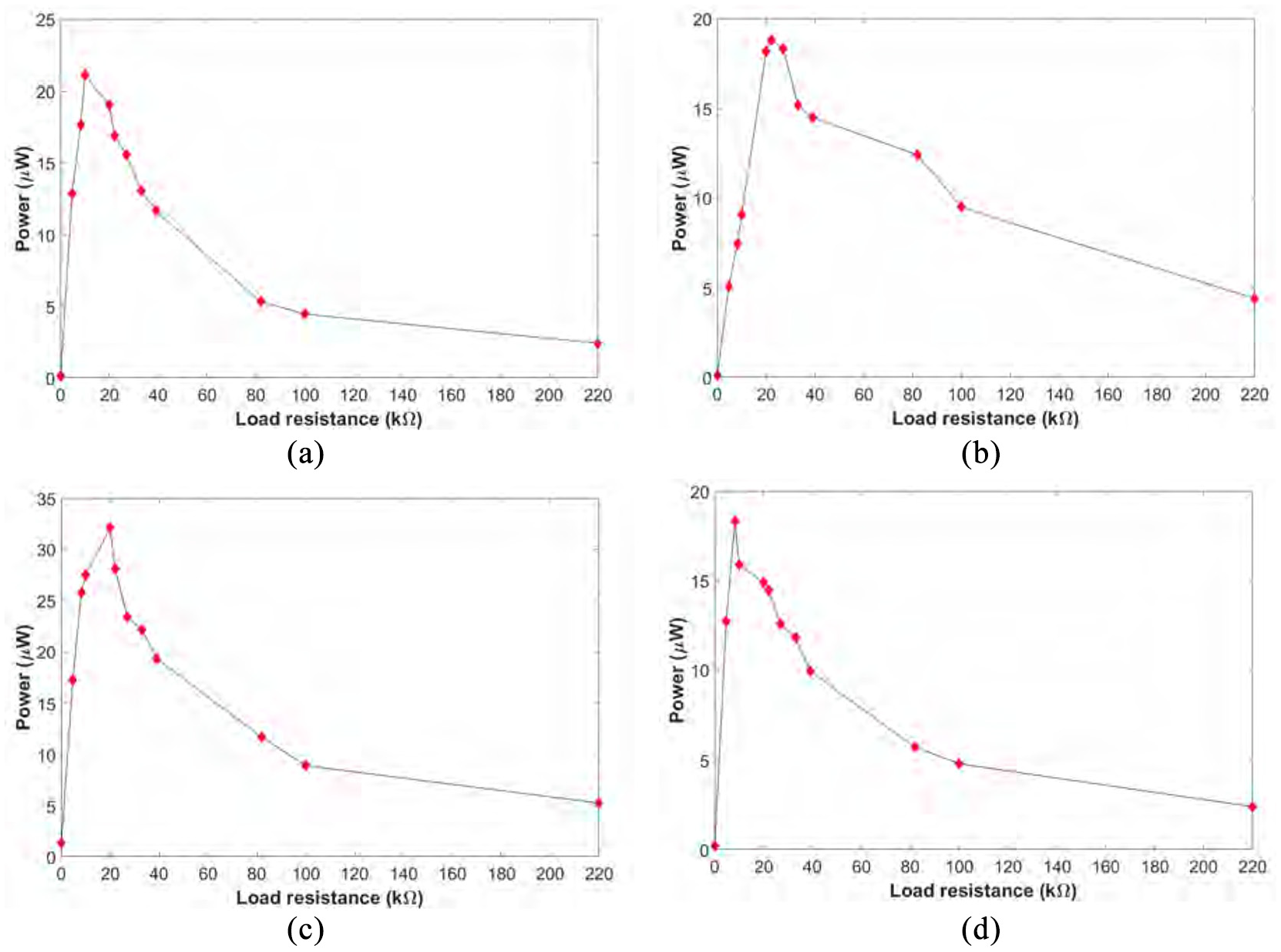
Average power generated by the piezoelectric beam at aft wall for various natural frequencies: (a) beam natural frequency = 332 Hz (CM2), (b) beam natural frequency = 108 Hz (CM3), (c) beam natural frequency = 228 Hz (CM3) and (d) beam natural frequency = 356 Hz (CM3).
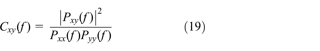
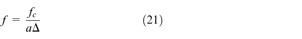
Coherence between the signals obtained from the piezoelectric beam and microphone throws light on how the beam and flow interact at different frequencies. For this, the magnitude-squared coherence,
where
Figure 22(a) shows the coherence thus plotted between the microphone signals at the front wall and aft wall of CM2 versus the piezoelectric beam placed at the aft wall. It can be noticed that the coherence value between the aft wall microphone and the beam is almost equal for both
where
where
Magnitude squared coherence between signals from microphone and piezoelectric beam: (a) beam at 332 Hz versus microphone signals (CM2), (b) beam at 108 Hz versus microphone signals (CM3), (c) beam at 228 Hz versus microphone signals (CM3) and (d) beam at 356 Hz versus microphone signals (CM3).
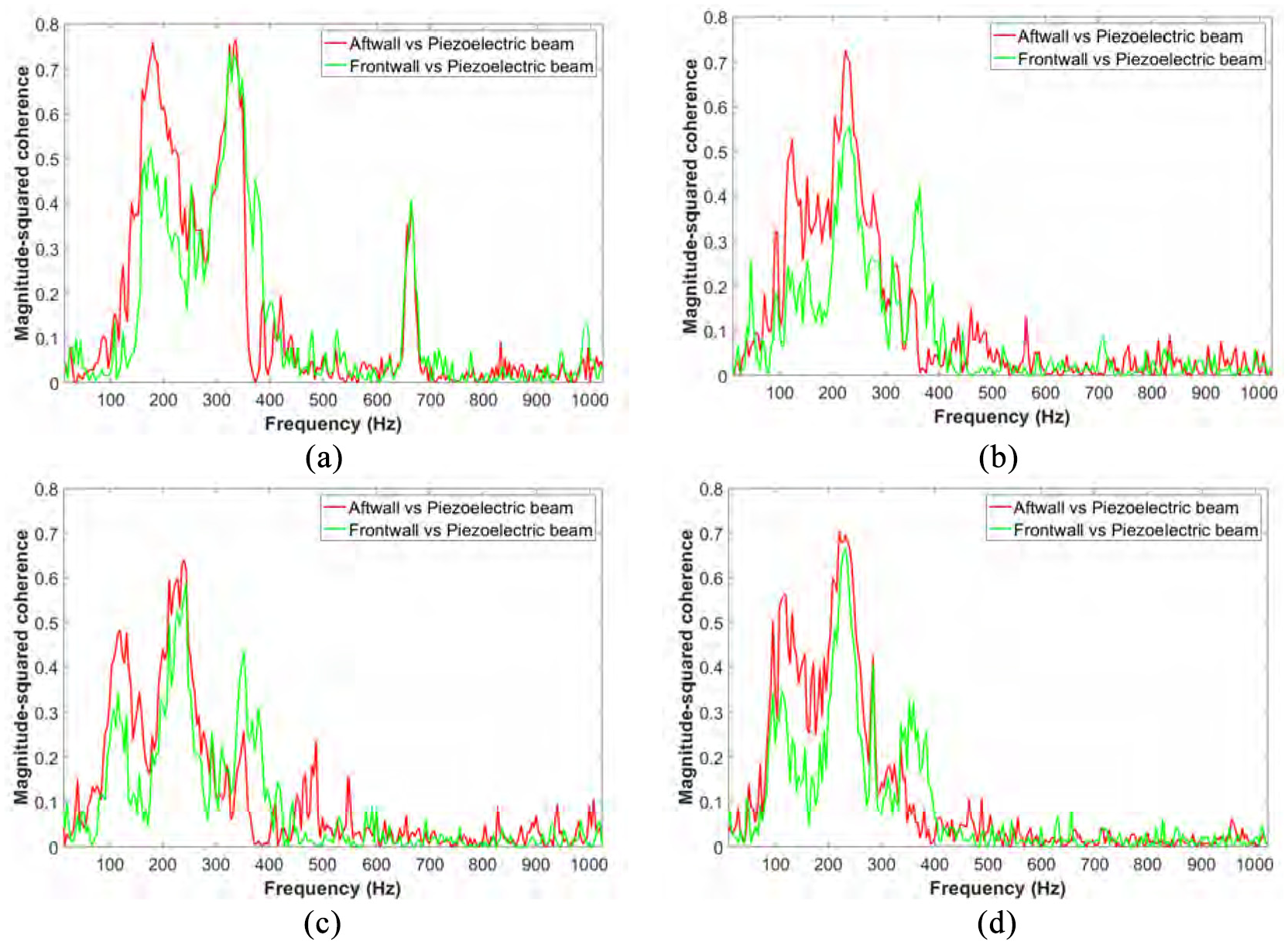
Normalized wavelet coefficients of signals from aft wall microphone and piezoelectric beam (at natural frequency = 332 Hz) for CM2: (a) aft wall microphone and (b) piezoelectric beam at aftwall.
For CM3, three different values of
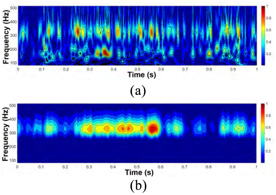
Variation of instantaneous voltage and power across the measurement time for CM3 when
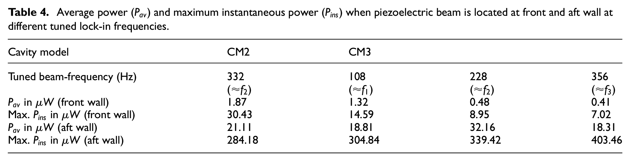
Average power (
6. Conclusion
The energy harvesting prospects of cavity flow oscillations were investigated by considering two different cavity geometries of L/D = 2 and 3 with an incoming flow of 30 m/s. The frequency spectra of the baseline cavities, obtained using microphones, showed high amplitude frequencies corresponding to Rossiter’s model. While the second mode of oscillation dominated for the cavity with L/D = 2, both the second and third mode of oscillation co-dominated for the cavity with L/D = 3. To harvest the oscillatory energy at these frequencies, a piezoelectric beam was tuned to match its natural frequency with them closely. The piezoelectric beam was located perpendicularly to the aft wall of the cavity at a distance of 0.22D from the trailing edge, which was shown by CFD results to be a region of highly fluctuating pressure levels. Average power of 21.11 µW and maximum instantaneous power of 0.28 mW was recorded for the cavity with L/D = 2 when the piezoelectric beam was tuned to the dominant frequency. For the cavity with L/D = 3, an average power of 32.16 µW and peak power of 0.34 mW was recorded for its dominant mode of oscillation. Coherence study between the fluctuating pressure and the piezoelectric signal showed a high value of coherence at the cavity frequencies. The time-frequency study of the signals using wavelet analysis showed that the cavity modes switched between the different active modes. When the cavity mode switched to the frequency closer to the natural frequency of the piezoelectric beam, high amplitudes of voltage was recorded.
The study highlights the promise that self-sustained cavity flow oscillations hold from an energy harvesting perspective. An additional encouraging factor is the presence of multiple dominant frequencies at which energy can be harvested, as opposed to several other methods employed in harvesting flow-induced vibrations, wherein only a single dominant forcing frequency is available. There also is much scope to improve the energy harvested by this method since in the current study it was seen that the energy harvester was yielding trivial power when the frequency of cavity flow oscillation differed from its natural frequency.
Footnotes
Appendix 1
Acknowledgements
We wish to gratefully acknowledge and thank the Government of Malaysia for supporting this work.
The authors also acknowledge the use of the IRIDIS High Performance Computing Facility at the University of Southampton, UK, in the completion of this work.
Declaration of conflicting interests
The authors declared no potential conflicts of interest with respect to the research, authorship, and/or publication of this article.
Funding
The authors disclosed receipt of the following financial support for the research, authorship, and/or publication of this article: This research was supported by the Ministry of Higher Education (MoHE), Malaysia, through the Fundamental Research Grant Scheme FRGS/1/2018/TK10/USMC/03/1.