Sage Journals: Discover world-class research

Abstract

Many structural aspects of music, such as tonality, can be expressed using hierarchical representations. In music analysis, so-called keyscapes can be used to map a key estimate (e.g., C major, F minor) to each subsection of a piece of music, thus providing an intuitive visual representation of its tonality, in particular of the hierarchical organization of local and global keys. However, that approach is limited in that the mapping relies on assumptions that are specific to common-practice tonality, such as the existence of 24 major and minor keys. This limitation can be circumvented by applying the discrete Fourier transform (DFT) to the tonal space. The DFT does not rely on style-specific theoretical assumptions but only presupposes an encoding of the music as pitch classes in 12-tone equal temperament. We introduce wavescapes, a novel visualization method for tonal hierarchies that combines the visual representation of keyscapes with music analysis based on the DFT. Since wavescapes produce visual analyses deterministically, a number of potential subjective biases are removed. By concentrating on one or more Fourier coefficients, the role of the analyst is thus focused on the interpretation and contextualization of the results. We illustrate the usefulness of this method for computational music theory by analyzing eight compositions from different historical epochs and composers (Josquin, Bach, Liszt, Chopin, Scriabin, Webern, Coltrane, Ligeti) in terms of the phase and magnitude of several Fourier coefficients. We also provide a Python library that allows such visualizations to be easily generated for any piece of music for which a symbolic score or audio recording is available.

Keywords

Discrete Fourier transform music analysis keyscapes tonal hierarchy visualization

Many domains of human cognition, such as music, language and action planning, exhibit hierarchical structure (Arbib, 2013; Rebuschat et al., 2012). In the case of music, several structural features are organized hierarchically, for instance formal arrangement, rhythm, melody and tonality (Abdallah et al., 2016; Caplin, 1998; Gilbert & Conklin, 2007; Mavromatis, 2012; Rohrmeier & Neuwirth, 2015). This article is concerned with the tonality of Western music, considered in a broad sense as the hierarchical organization of chords, scales and keys in pieces of music. Accordingly, notes can be grouped into chords that can be grouped into local keys that, in turn, are grouped into the global key of a piece. For instance, a classical piece could be in the key of C major, globally, but at the same time have subordinate sections in related keys such as G major and A minor. On an even more local level, more frequent changes of harmony can occur, for instance through applied dominant chords (e.g., A7, the dominant of D minor).

This article proposes a new approach to the visualization of hierarchical tonal structures. As demonstrated by several case studies, the method goes beyond related techniques in that it is applicable to a wide range of Western musical styles, including the extended tonality of the 19th century. In the following, we first summarize the related research that motivates our approach.

In music analysis, Schenkerian theory aims at revealing hierarchical relations between musical elements in order to derive a complete reduction of a piece (Cadwallader & Gagné, 1998). Such relations can be studied using frameworks from formal language theory (Manning & Schütze, 2003), and there have been many attempts to formalize Schenkerian’s intuitions (e.g., Lerdahl & Jackendoff, 1983), in particular by employing formal grammars that represent hierarchical relations within sequences of notes or chords (Abdallah et al., 2016; Keiler, 1978; Kirlin & Jensen, 2011; Rohrmeier, 2011; Steedman, 1984). Such mathematical models bridge the gap between music theory and psychology by describing human cognition on the computational level (Harasim, 2020; Marr, 1982).

However, there are theoretical and practical difficulties for automatic hierarchical music analysis. For instance, the combinatorial complexity of deciding between all plausible relations for a given musical sequence might cause long computation times or even render the decision intractable for long pieces such as entire sonatas or symphonies. Furthermore, representing the hierarchical relations in a piece of music using formal grammars requires a set of generative rules that model the syntax of a musical style. However, virtually all approaches to musical grammar focus on the so-called common-practice tonality (Rohrmeier & Neuwirth, 2015; Tymoczko, 2003), blues (Katz, 2017; Steedman, 1996), or jazz (Granroth-Wilding & Steedman, 2012; Harasim et al., 2018, 2019; Rohrmeier, 2020). Many other forms of tonality that go beyond these idioms have not been studied sufficiently from the formal language perspective, for instance Renaissance modality or late 19th-century extended tonality. Formal grammars do not exist for these styles—at least not to date.

Visual hierarchical music analysis

Keyscapes (Sapp, 2001, 2005) provide an alternative approach to hierarchical music analysis. They visualize key estimates for all possible subdivisions of a piece (see e.g., Figure 1). Those estimates are commonly obtained by a key-finding algorithm that returns the best-fitting major or minor key according to the distribution of notes in a segment of music (Krumhansl, 1990; Temperley, 1999). Keyscapes require much less computation than, for instance, formal grammar models and can be viewed as a first approximation for the hierarchical organization of the tonal material in a musical composition or improvisation.

Figure 1.

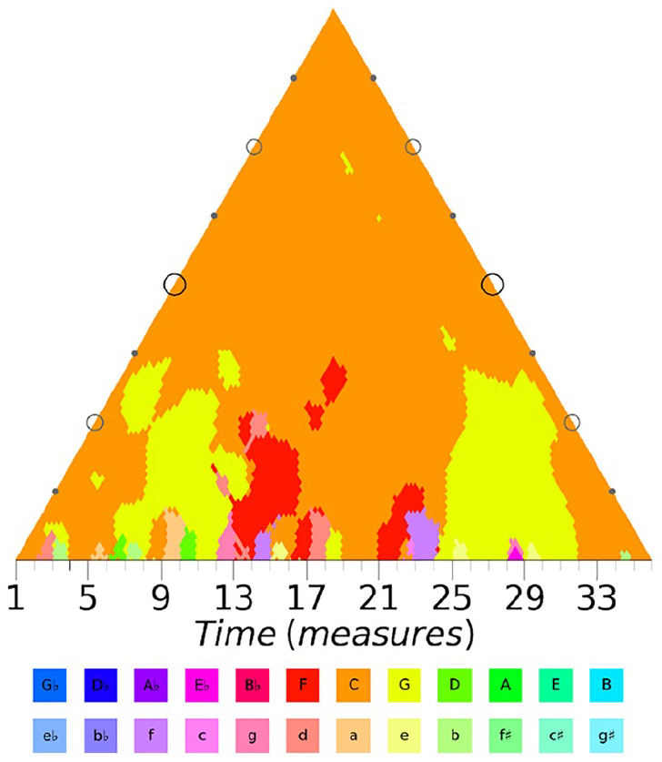
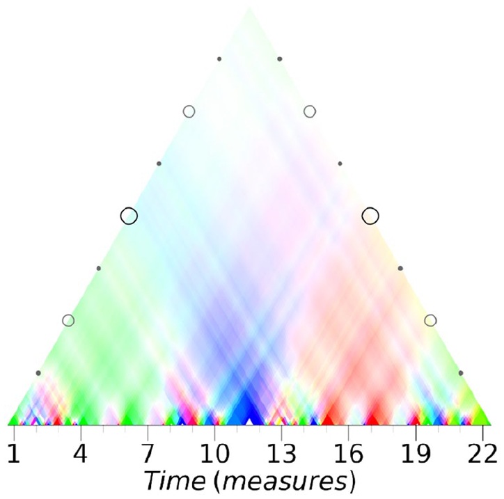
Keyscape of Bach’s Prelude in C major (BWV 846).

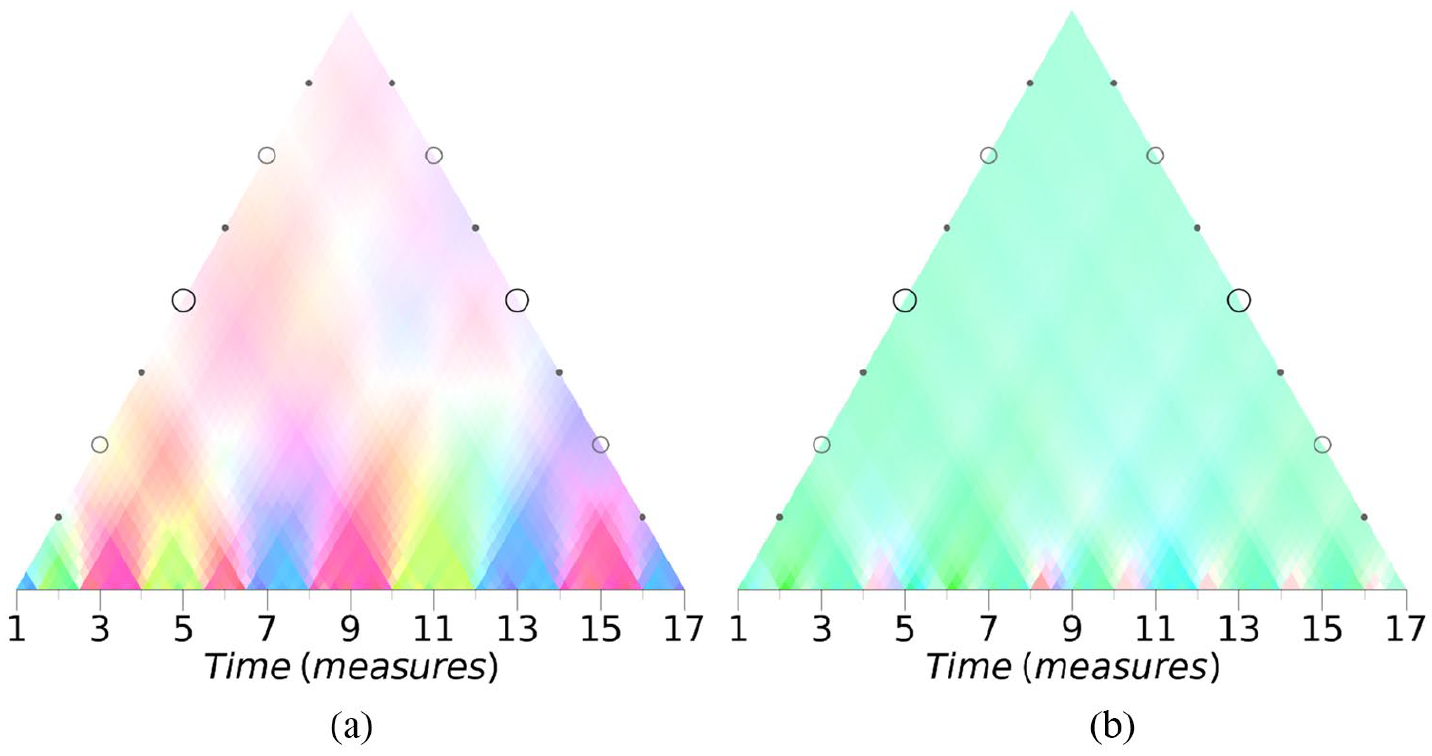
As an example, Figure 1 shows the keyscape for Bach’s Prelude in C major (BWV 846) using the Krumhansl-Schmuckler key-finding algorithm (Krumhansl, 1990).¹ The mapping from key estimates to colors is displayed under the keyscape, with major and minor keys being arranged along the circle of fifths. The markers on the sides of the triangle indicate different segments of the piece, and the bar numbers are shown under the keyscape. The figure shows that the algorithm produces different key estimates for different parts of the piece. The keyscape thus represents the algorithm’s estimation of the prelude’s local key regions and modulations. The global key is correctly estimated as C major (shown in orange), and large subsections are attributed to F major (shown in red) and G major (shown in mustard yellow). These subordinate key sections represent modulations to the subdominant and dominant keys that are common in Baroque pieces. The example demonstrates how keyscapes can be used to visualize the hierarchical organization of keys in a composition. Although this visualization does not explicitly provide a tree- or graph-structured analysis of the music, it is a useful tool for music analysis that is easy to understand for a broad audience.

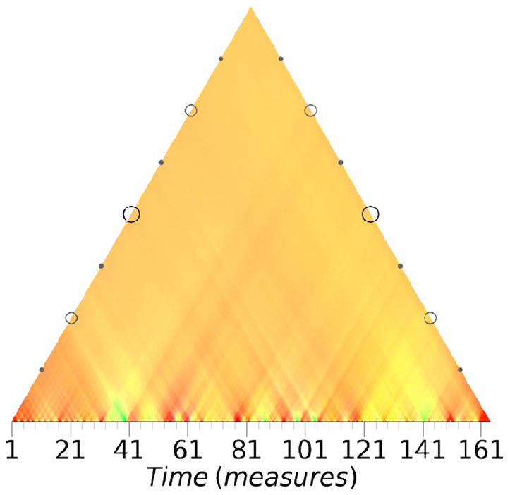
It is tempting to apply keyscapes also to pieces from musical styles other than common-practice tonality or jazz. However, that approach does not always lead to satisfying results (Sapp, 2005). Figure 2 shows the keyscape for the introduction of Liszt’s Faust Symphony (S. 108). According to the key-finding algorithm’s estimate, the introduction is in the key of F minor, with the first and second half being in C♯ minor and A minor, respectively. We discuss the tonality of this piece in more detail below (see “Analytical case studies”). Here, we want to point out that an analysis that relies on major or minor keys does not do justice to its intricate harmonic structure (Cohn, 2012). An appropriate analysis of tonality in late 19th-century music, sometimes referred to as “extended tonality” (Schoenberg, 1969), requires more advanced concepts, such as chromaticism, extended harmonies, and symmetrical chords and scales (Cohn, 1996; Haas, 2004; Horton, 2018; Kopp, 2002; Lerdahl, 2001; Lieck et al., 2020; Polth, 2018; Weiß & Habryka, 2014). Thus, keyscapes based on key-finding algorithms are not suitable for representing extended tonality. Nonetheless, the abstract idea of visualizing hierarchical structures remains applicable because it is independent of the tonal content of a piece. In fact, the hierarchical representation of keyscapes can also be used for other applications, such as the study of timbre, tempo variations in different performances of the same piece, and melodic similarity (Park et al., 2019; Sapp, 2007; Segnini & Sapp, 2005).

Figure 2.

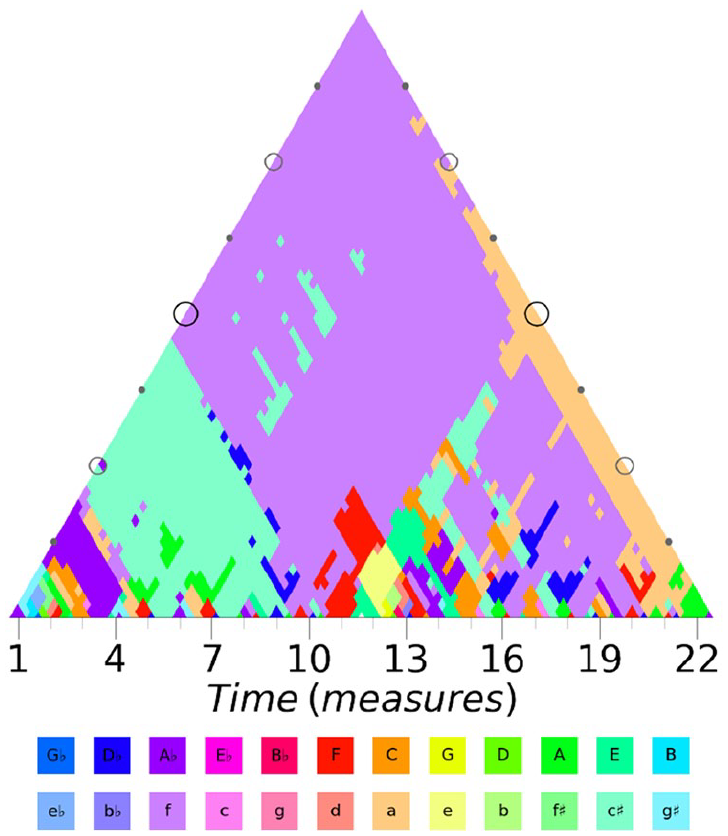
Keyscape of the opening of Liszt’s Faust Symphony (S. 108).

Analysing music using the discrete Fourier transform (DFT)

Based on a rediscovered observation by Lewin (1959), music theorists have recently begun to analyze pieces by applying the discrete Fourier transform (DFT) to pitch-class sets (Amiot, 2016). The DFT transforms a set of pitch classes into complex numbers that describe characteristics of the music (Quinn, 2006, 2007). Since the DFT measures the prevalence of even divisions of the octave in pitch-class sets (Amiot, 2007), it is not based on major and minor keys and thus particularly useful for the analysis of extended tonality. Details of the DFT and its interpretations with respect to music are provided below (see “Methodology” and “Prototypes and their interpretation”).

The DFT has been used to analyze and compare the tonal languages of several composers, including Bach, Schubert and Scriabin (Noll, 2019; Yust, 2015), as well as existing approaches to key finding (Yust, 2017). It has also been applied to the study of changes in pitch-class distributions, both within pieces (Harding, 2020) and between compositions from different historical periods (Yust, 2019b). Moreover, several connections have been drawn between the DFT of pitch-class sets and geometric approaches to harmony such as voice-leading spaces (Hoffman, 2008; Tymoczko, 2008; Tymoczko & Yust, 2019) and the Tonnetz (Yust, 2019a).

The present approach

The motivation for this study is the observation that keyscapes are insufficient for pieces with non-standard tonal organization (see Figure 2), because the notion of a diatonic key is not equally applicable to pieces from all time periods or styles. In contrast, the method proposed in this article does not rely on the concept of musical keys but only on the representation of tones as pitch classes and thus reveals the tonal structure of a piece in a more general way.

Our approach combines the hierarchical representation of keyscapes with the analytical insights obtained from the application of the DFT to pitch-class sets. Since keyscapes depict different hierarchical levels of tonality in a piece of music but have the shortcoming that they rely on a diatonic key-finding algorithm as mentioned above, we substitute such algorithms by outputs of the DFT and use a color mapping that exploits geometric properties of the Fourier space. We thus obtain a visual depiction of the hierarchical relations of tonal structures in a piece. Because the DFT measures periodicity in a signal by means of combinations of cosine and sine waves, we call the resulting visualization wavescapes. The synthesis of these two methods advances computational musicology by providing an elegant visualization that is a first building block in the deeper understanding of hierarchical relations in music not only within but also beyond common-practice tonality.

Recently, Lieck and Rohrmeier (2020) introduced pitch scapes, which employ a Fourier representation to directly model prototypical hierarchical pitch-class statistics independently of any key-finding algorithms. However, the visualization of the results was again performed using conventional key-finding algorithms. Their approach can therefore be considered complementary to ours and wavescape visualizations might facilitate the interpretability of pitch scapes.

In the remainder of this article, we first provide a detailed description of the DFT, its application to pitch-class sets, and an intuitive color mapping to create wavescapes (“Methodology”). We then discuss a number of prototypical examples (“Prototypes and their interpretation”). In the following section (“Analytical case studies”), we analyze eight pieces of music and demonstrate how wavescapes can provide insights into the tonal structures in these pieces. Finally, we discuss the benefit of using wavescapes for music analysis more generally and point out several potential extensions of our approach, before concluding with some final remarks.

Methods

This section starts by describing how pieces of music can be transformed into a hierarchy of pitch-class vectors. Then, we describe the discrete Fourier transform (DFT), its application to such hierarchies, and the color mapping used for the obtained Fourier coefficients. This procedure results in a visual representation of pieces called wavescapes.

A hierarchy of pitch-class vectors

We start by partitioning a piece of music into $N$ non-overlapping segments of equal length $r$ . In this general sense, segments can be defined by musical units in symbolic scores (e.g., measures, note durations) as well as by continuous durations in audio recordings (e.g., seconds, onsets).² In the present study, we chose appropriate resolutions $r$ according to the time signatures of the pieces (see “Analytical case studies”). The $q$ -th segment of a piece is represented by a pitch-class vector (PCV) $x_{q} \in ℝ_{\geq 0}^{12}$ (1 ≤ q ≤ N) whose entries contain the total durations (also called weights) of the 12 pitch classes in that segment. A pitch class is the equivalence class of all octave-related pitches in 12-tone equal temperament (C, C♯, D, D♯, E, F, F♯, G, G♯, A, B♭, B), assuming enharmonic equivalence. The value $x_{q} [0]$ is the weight of pitch class C, $x_{q} [1]$ is the weight of C♯, and so forth. For example, the PCV of the first four measures of J. S. Bach’s Prelude in C major shown in Figure 3 is $x = (14, 0, 9, 0, 9, 2, 0, 3, 0, 1, 0, 4)$ , where the duration of each pitch class is given in quarter-notes.

Figure 3.

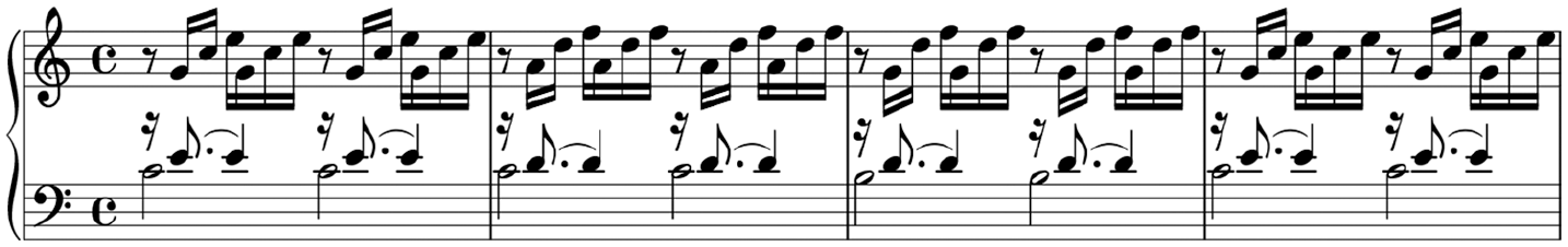
The first four bars of Bach’s Prelude in C major.

A complete piece is modeled as a hierarchy of segments given by a function $p$ that inclusively returns the pitch-class content from the $m$ -th to the $n$ -th segment,

P : ℕ^{2} \to ℝ_{\geq 0}^{12}, (m, n) \mapsto \sum_{q = m}^{n} x_{q},

(1)

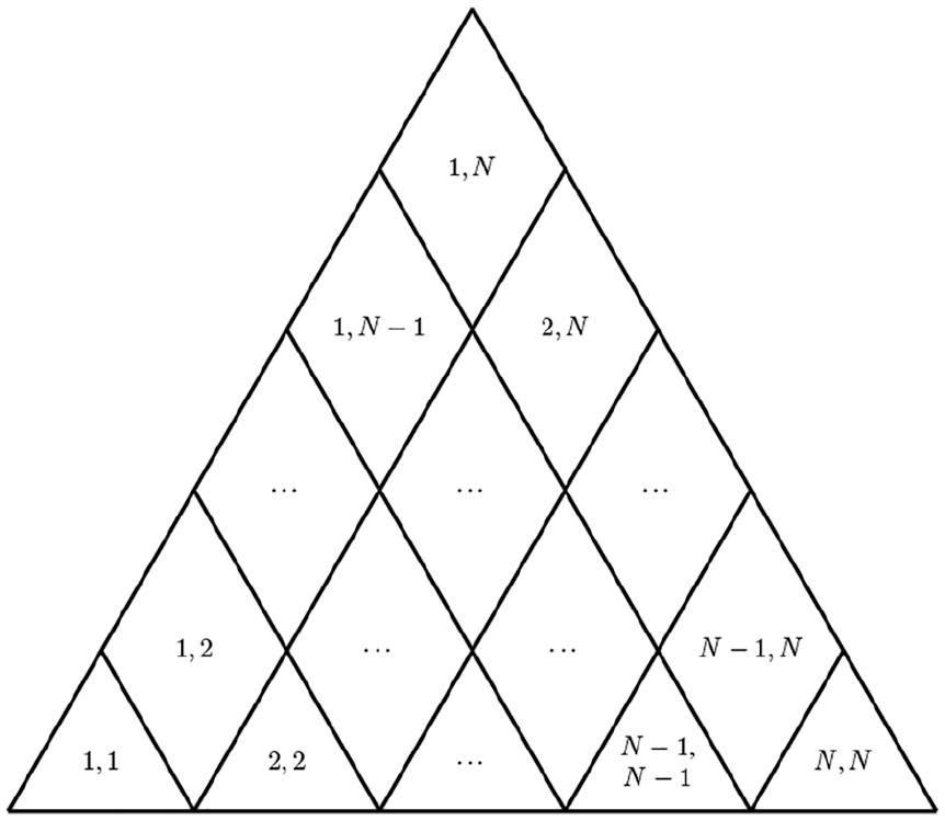
for (1 ≤ m ≤ n ≤ N). The size as well as the hierarchical level of the $(m, n)$ -th segment is then $n - m + 1$ , and there are $\sum_{q = 1}^{N} q = \frac{N (N + 1)}{2}$ segments in total. This hierarchy is shown schematically in Figure 4, where all cells are represented as diamonds (except those at the very bottom which are shown as triangles).

Figure 4.

Visualization of the hierarchy of segments given by $P$ .

Discrete Fourier transform

The DFT decomposes a vector into a sum of sinusoidal functions of unique frequency with varying amplitudes and phases. That is, the DFT of any PCV $x$ is the mapping

F : ℝ_{\geq 0}^{12} \to ℂ^{12}, x \mapsto X,

(2)

where the $k$ -th component of the complex-valued vector $X$ is given by

X [k] = \sum_{n = 0}^{11} x [n] e^{- i 2 π n \frac{k}{12}}

(3)

for $k \in [0, \dots, 11]$ . The values of $X [k]$ are referred to as Fourier coefficients, or simply coefficients. The zeroeth coefficient $X [0]$ is always equal to the sum of $x$ . By symmetry, the coefficients for $k \in [1, \dots, 5]$ are conjugate to the ones for $k \in [11, \dots, 7]$ while the sixth coefficient is its own conjugate, $X [k] = \bar{X} [12 - k]$ for $k \in [1, \dots, 11]$ . Therefore, we consider only the coefficients 1 to 6 in accordance with previous research (Amiot, 2007; Yust, 2019a).

Since Fourier coefficients are complex numbers, they can be described in polar coordinates by their magnitude µk (i.e., the distance to zero) and their phase $ϕ_{k}$ (i.e., the angle in counterclockwise orientation starting from 3 o’clock),

X [k] = μ_{k} \cdot e^{i ϕ_{k}}

(4)

Consider for instance again the PCV of the example shown in Figure 3, $x = (14, 0, 9, 0, 9, 2, 0, 3, 0, 1, 0, 4)$ . Its fifth Fourier coefficient $X [5]$ has phase $ϕ_{5} = 0.29 π$ , and magnitude µ₅ =24.19.

Color mapping of Fourier coefficients

To visualize the Fourier coefficients of PCVs, we represent them in polar coordinates and map their phases and magnitudes to colors. Given the periodic nature of the phase, it can be assigned to a color through a circular hue. We choose the hue function $h : [0, 2 π [\to {[0, 1]}^{3}$ that maps $ϕ_{k}$ to a triple $(r, g, b)$ , representing the strengths of the red, green and blue components of the color (Ong & Khoo, 2014):

h (ϕ_{k}) = {\begin{cases} (1, \frac{3 ϕ_{k}}{π}, 0) if 0 \leq ϕ_{k} < \frac{π}{3} \\ (2 - \frac{3 ϕ_{k}}{π}, 1, 0) if \frac{π}{3} \leq ϕ_{k} < \frac{2 π}{3} \\ (0, 1, \frac{3 ϕ_{k}}{π} - 2) if \frac{2 π}{3} \leq ϕ_{k} < π \\ (0, 4 - \frac{3 ϕ_{k}}{π}, 1) if π \leq ϕ_{k} < \frac{4 π}{3} \\ (\frac{3 ϕ_{k}}{π} - 4, 0, 1) if \frac{4 π}{3} \leq ϕ_{k} < \frac{5 π}{3} \\ (1, 0, 6 - \frac{3 ϕ_{k}}{π}) if \frac{5 π}{3} \leq ϕ_{k} < 2 π \end{cases}

(5)

This color mapping is visualized in Figure 5.

Figure 5.

Color space defined by the color mapping $C^{k}$ .

The magnitude µ_k of a Fourier coefficient can be mapped to an opacity³ value $α = μ_{k} / X [0]$ by normalizing it with the sum of PCV $x$ , given by its zeroeth coefficient $X [0]$ .⁴ The normalization of the magnitude also facilitates the comparison of different PCVs with one another.

We represent the phase and magnitude mappings by a coloring function $C_{k}$ ,

C_{k} : ℂ^{12} \to {[0, 1]}^{3} \times [0, 1], X \mapsto ((r, g, b), α),

(6)

which selects the $k$ -th coefficient of $X$ and uses the previous mappings on its phase and magnitude to return a color:

C_{k} (X) = (h (ϕ_{k}), \frac{μ_{k}}{X [0]})

(7)

Wavescapes

In summary, a pitch-class vector can be colored by successively applying the DFT $F$ and the coloring $C_{k}$ . Together with $P$ , these mappings define an arrangement of colors for a given piece of music that we call a wavescape. More precisely, the wavescape for the $k$ -th Fourier coefficient is expressed by

W_{k} : ℕ^{2} \to {[0, 1]}^{3} \times [0, 1], W_{k} [m, n] = (C_{k} \circ F \circ P) [m, n],

(8)

for segment indices $m, n \in ℕ$ with 0 ≤ m ≤ n < N. According to the hierarchical structure shown in Figure 4, wavescapes are displayed as colored triangles similar to keyscapes (see Figures 1 and 2).

There are six wavescapes for any given piece (one per Fourier coefficient, $k \in [1, \dots, 6]$ ) and each of them may show interesting properties for music analysis. In order to determine on which wavescape to concentrate our analyses, we focus on those with the largest average normalized magnitude (denoted by ${\bar{α}}_{k}$ for coefficient $k$ ) in the section “Analytical case studies.”

In connection with this article, we provide an implementation of the methods described above in a Python library that is freely available at https://github.com/DCMLab/wavescapes. It can be used to reproduce the results in this study and, more generally, to generate wavescape plots from MIDI, MusicXML or audio input. See the README file for more instructions.

Prototypes and their interpretation

The previous section presented how a PCV can be mapped to six colors that visualize the phase and normalized magnitude of its Fourier coefficients. In this section, we describe how those colors are interpreted with respect to the music in order to explain the role of the DFT in music theory. We begin by investigating a number of music-theoretically relevant pitch-class sets and scales (Harasim et al., 2021). A pitch-class set $y = {y_{1}, \dots, y_{m}}$ is a set of any number of the 12 pitch classes. The D minor triad is for example given by ${2, 5, 9}$ . We represent pitch-class sets by a PCV $x \in {0, 1}^{12}$ in which ones and zeros indicate the presence and absence of pitch classes, respectively. Thus, the D minor triad is represented by the PCV $x = (0, 0, 1, 0, 0, 1, 0, 0, 0, 1, 0, 0)$ .

For any pitch-class set, the (normalized) magnitudes of the DFT are invariant under transposition and inversion (Amiot, 2016). To describe the intuition behind such magnitudes, we therefore consider equivalence classes of pitch-class sets under transposition and inversion, such as scales, triads and symmetric chords (e.g., augmented triads and fully diminished chords), and call them set classes (Forte, 1977).

The normalized magnitudes of selected set classes are shown in Figure 6. Notably, the normalized magnitudes $α$ are maximal ( $α = 1$ , black) for some combinations of pitch-class sets and coefficients, and minimal ( $α = 0$ , white) for others. The pitch-class sets that maximize the normalized magnitudes suggest how the respective Fourier coefficients representing the music can be interpreted. For example, tritones maximize the normalized magnitudes for $k = 2, 4, 6$ , augmented triads for $k = 3, 6$ , fully-diminished chords for $k = 4$ , and finally whole-tone scales for $k = 6$ . The normalized magnitudes of all coefficients are moreover maximal for singleton sets.

Figure 6.

Normalized magnitudes of the Fourier coefficients for different chords and scales.

In general, the normalized magnitude of the $k$ -th coefficient is maximal for binary PCVs $x$ that represent an equal division of the octave if the number of its non-zero components is a common divisor of $k$ and 12. Quinn (2006, 2007) calls these PCVs prototypes.⁵ Since only the coefficients 1 through 6 are considered (see “Methodology”), the fifth coefficient is the only one whose index ( $k = 5$ ) cannot be divided evenly by $12$ (Clough & Douthett, 1991). Therefore, its normalized magnitude is maximized only by singletons.

Figure 6 shows a variety of non-prototypical set classes as well. For instance, major and minor triads have rather large but not maximal values for coefficients $k = 3, 4, 5$ . The normalized magnitudes of the dominant-seventh and half-diminished chords are largest for the fourth coefficient, while the normalized magnitude for the major seventh chord is largest for the third coefficient. For all coefficients, the magnitude of the chromatic pitch-class set $Ω = (1, 1, 1, 1, 1, 1, 1, 1, 1, 1, 1, 1)$ equals $0$ .

Some symmetrical scales also suggest interpretations of the Fourier coefficients whose magnitudes they maximize.⁶ For instance, hexatonic scales such as $H_{0, 3} = (1, 0, 0, 1, 1, 0, 0, 1, 1, 0, 0, 1)$ have a non-zero magnitude only for the third coefficient while octatonic scales such as $O_{0, 1} = (1, 1, 0, 1, 1, 0, 1, 1, 0, 1, 1, 0)$ are non-zero only for the fourth coefficient (see Figure 6). The whole-tone scale, as mentioned before, is non-zero and maximal for the sixth coefficient. Observing large magnitudes on the wavescapes for those coefficients suggests that the corresponding segments of a piece are largely organized by these particular scales.

We use the following notation for the prototypes: $H_{i, j}$ is a hexatonic scale, $O_{i, j}$ is an octatonic scale, $W T_{i}$ is a whole-tone scale, and $T_{i}$ is a tritone, where $i, j$ refer to non-zero pitch-classes that these pitch-class vectors contain. Diatonic scales (major and natural minor) are denoted by the number of flats and sharps in their key signatures, for instance 3♭ for E♭ major/C minor, ♮ for C major/A minor, and 2♯ for D major/B minor (Gárdonyi & Nordhoff, 2002). Augmented triads are notated as C+, D+, etc., and diminished seventh chords as Cº⁷, Dº⁷, etc.

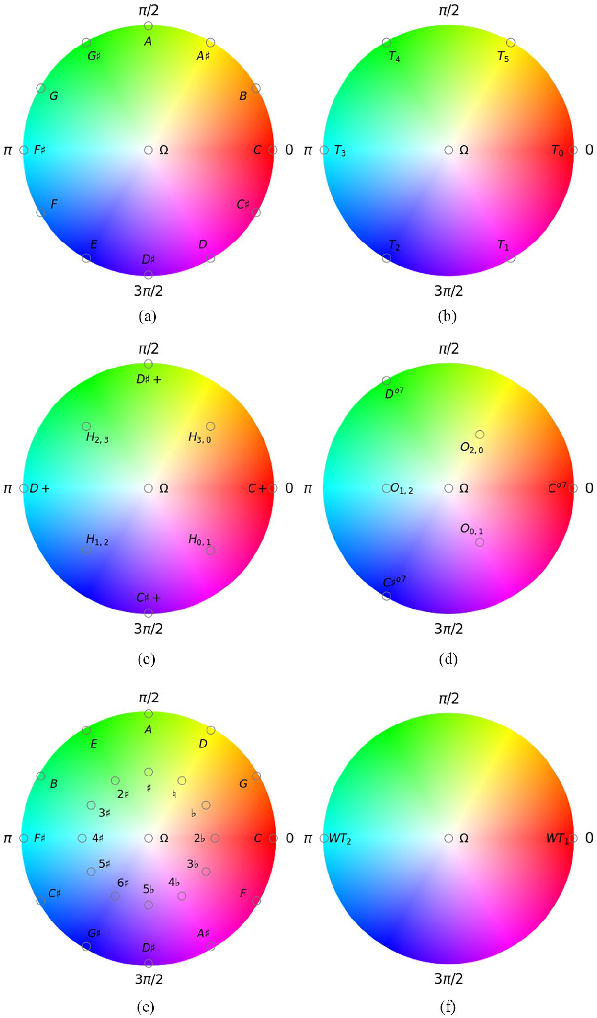
Because the magnitudes are identical for all members of a set class, it is interesting to observe how the phases of these members change. The transposition of a pitch-class set is directly related to a phase change. For example, transposing an augmented triad upwards by a semitone corresponds to a phase change of $+ \frac{π}{2}$ in the third coefficient (see Figure 7c).

Figure 7.

Prototypes for the different coefficients.

For each coefficient, Figure 7 shows how its prototypes and other relevant pitch-class sets are mapped to a magnitude, a phase, and thus, a color (see “Methodology”). Each subplot shows the chromatic pitch-class set Ω in the center. The DFT maps the phases of the singleton prototypes for the first coefficient to clockwise ascending chromatic order (top left), like the tritones for the second coefficient (top right). The prototypes of the third coefficient—the four augmented triads—are mapped onto the real and imaginary axes, and the hexatonic scales are mapped exactly between the two augmented triads that they contain (middle left). Analogously, for the fourth coefficient, the three fully diminished chords are the prototypes of the fourth coefficient and the three octatonic scales lie between their two constituting diminished chords (middle right). In the sixth coefficient, the two whole-tone scales are mapped to the real poles (bottom right).

A number of common musical scales such as the diatonic scale, the pentatonic scale, and Guido’s natural hexachord (Reisenweaver, 2013) are contiguous subsegments of the circle of fifths.⁷ The fifth coefficient maps these scales as well as the singletons along the circle of fifths in counter-clockwise ascending order (bottom left, only diatonic scales and singletons are shown). Note that each diatonic scale spans six fifths on this circle, for example B♭-F-C-G-D-E-A in the case of F major/D minor. Since G is its center on the circle of fifths, the phases for this diatonic scale and the singleton G are identical. The pitch-class sets of F major and D natural minor are mapped to the same point in the Fourier coefficients because they are identical (♭ ≡ $(1, 0, 1, 0, 1, 1, 0, 1, 0, 1, 1, 0)$ ). The larger cardinality of the diatonic scales leads to smaller normalized magnitudes than for the singletons and thus to brighter colors.

The tonal material of (segments of) actual pieces of music does not generally correspond to the prototypes that represent abstract music-theoretical concepts such as certain chords or scales. PCVs rather have small but positive weights for out-of-scale notes and larger weights for in-scale notes. Their highest weight is commonly at the local tonic. Figure 8 visualizes the fifth coefficients of all 24 major and minor keys, using the weights provided by Albrecht and Shanahan (2013). A comparison of Figures 7e and 8 shows how the fifth coefficient differs between diatonic scales and keys. The root and the fifth are particularly prominent in major and minor keys, and minor keys tend to be more chromatic due to the notes from the dominant key such as the leading tone. Therefore, minor keys are pulled away counter-clockwise from their scale, while major keys are pulled away in the clockwise direction.

Figure 8.

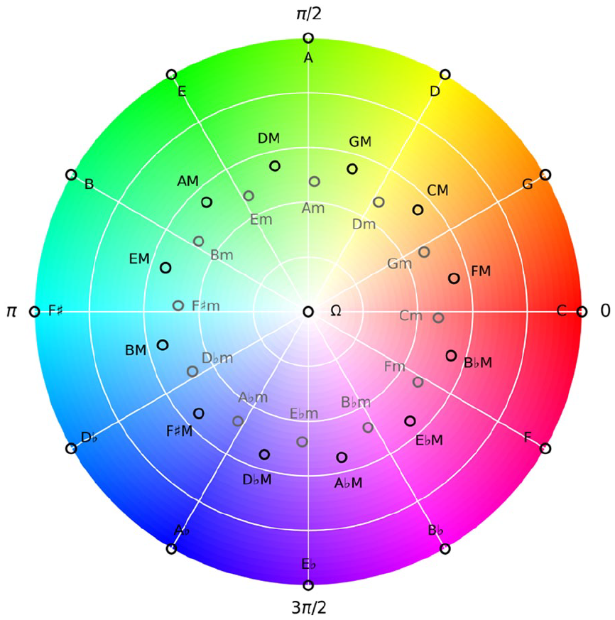
Fifth coefficients for diatonic major and minor keys.

In sum, the interpretations of the six coefficients resonate well with music-theoretical descriptions (Amiot, 2016; Lewin, 2001; Yust, 2019b) and empirical findings (Honingh & Bod, 2010, 2011), as the chromatic circle and the circle of fifths are fundamental structures for Western classical music and jazz (Aldwell et al., 2010; Rohrmeier, 2020). Furthermore, the highly dissonant harmonies of post- and atonal music (Straus, 2005) maximize magnitudes for the first two coefficients. In contrast, hexatonic and octatonic scales are in frequent usage in late Romantic music (Cohn, 2012; Lendvai, 1971), and the whole-tone scales are emblematic for 20th-century impressionism (Tresize, 2017).

Analytical case studies

To show the applicability and interpretability of wavescapes, we use them to analyze eight pieces, namely

Liszt’s Faust Symphony, S. 108

Josquin’s motet Ave Maria

Bach’s Prelude in C major BWV 846 no. 1

Chopin’s Prelude in A minor op. 28 no. 2

Scriabin’s Prelude op. 74 no. 2

Coltrane’s Giant Steps

Webern’s Variations for Piano no. 1

Ligeti’s Études pour Piano no. 2

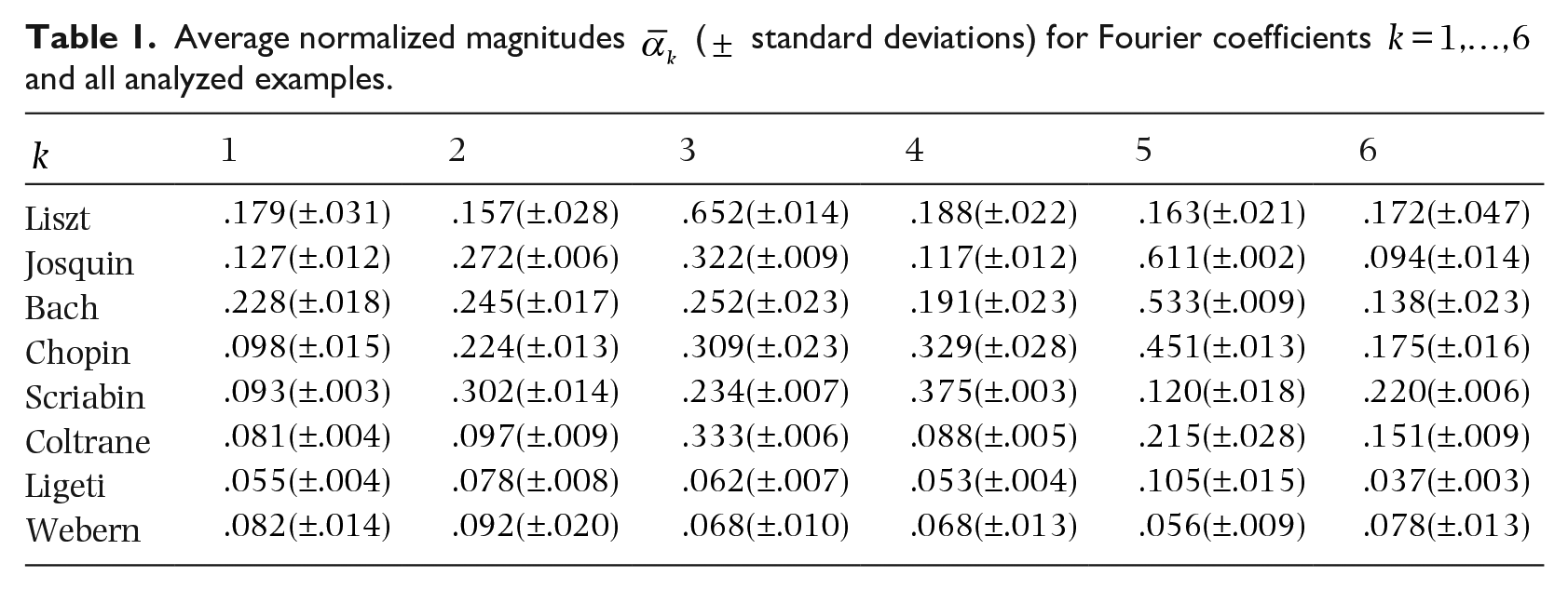
The examples are not presented in historical order; the focus of each case study is rather to highlight interesting analytical details of the individual pieces. Also, not all pieces are discussed at the same level of detail. The Faust Symphony is discussed most extensively. For the remaining case studies, we present selected observations and show only the corresponding wavescapes in the main text. The wavescapes for all six coefficients and all pieces are shown in Figures 19 –26 in the Appendix. Moreover, Table 1 in the Appendix shows the average normalized magnitudes for all pieces and coefficients.

Liszt’s Faust Symphony, S. 108

The opening of the first movement of Liszt’s Faust Symphony (bars 1–22, Lento assai, 4/4 time signature) presents harmonic material that reflects Liszt’s shift from a diatonic towards a chromatic conception of tonality during the second half of the 19th century.⁸ For the visualization in the wavescapes we chose a resolution of one quarter-note.

Previous analyses of this symphony likewise focus on the first movement and consider its global structure to be determined by three main pitches, C, E and A(Longyear & Covington, 1986), which together form the A♭augmented triad. Since augmented triads are not contained in the natural diatonic scale (Bribitzer-Stull, 2006; Weitzmann, 1853), keyscapes that rely on on diatonic key-finding algorithms do not generate a satisfying analysis of this piece (see Figure 2 and the discussion there).

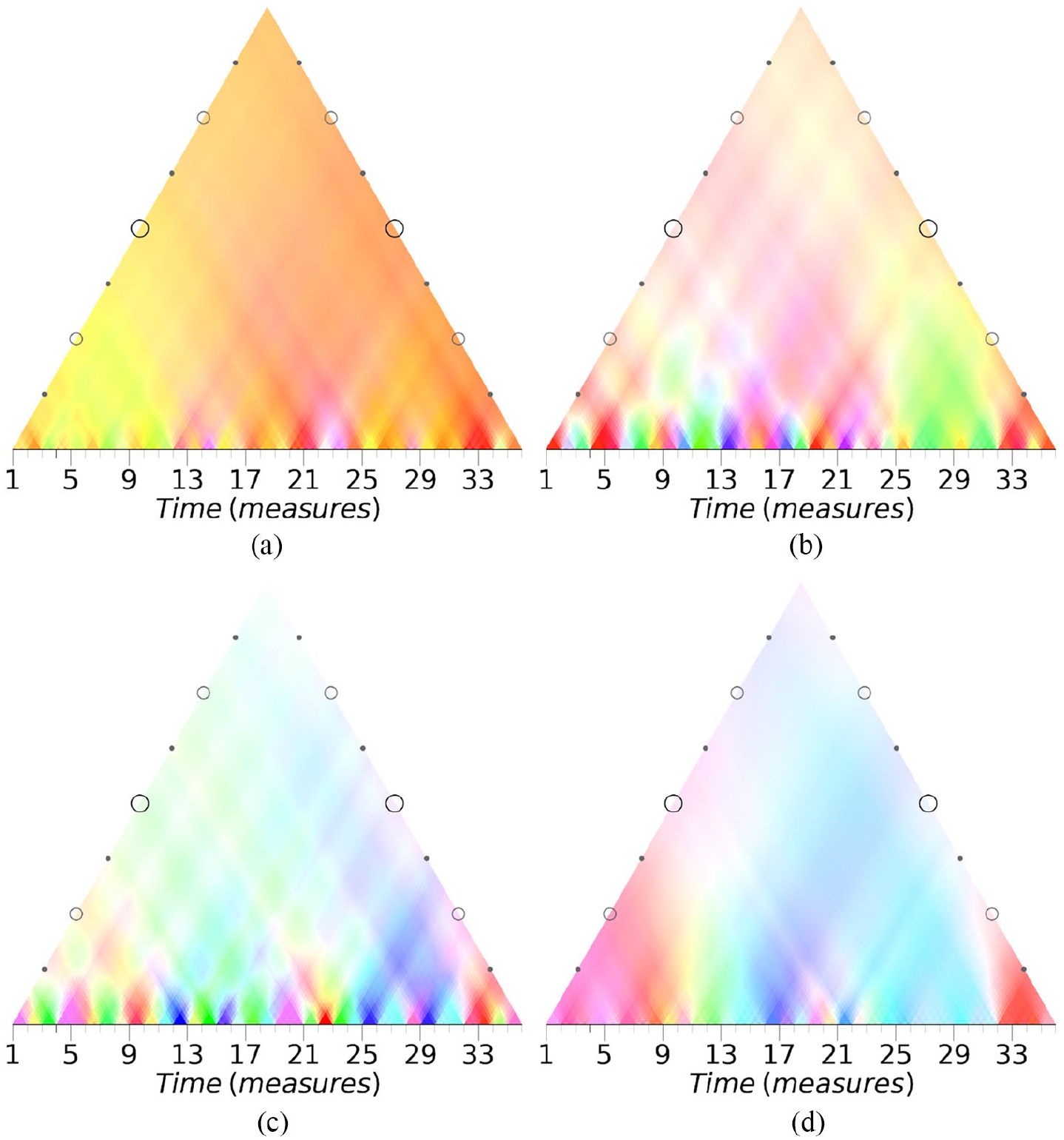
In contrast to Longyear and Covington (1986), Cohn (2012) and Argentino (2018) analyze the opening as an example for the usage of hexatonic scales, composed of the two augmented triads A♭-C-E and C♯-F-A. The wavescapes can help to evaluate these similar but different analyses. Augmented triads are prototypes for the third and sixth coefficient (see “Prototypes and their musical interpretation”). If the augmented triad were the most significant harmonic structure, one would expect maximal magnitudes for both the third and sixth coefficients (Figures 9a and 9b). 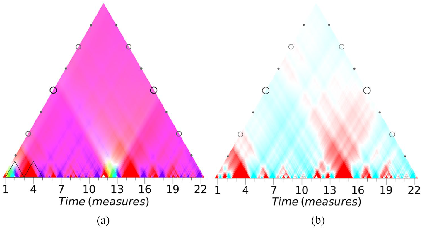A comparison of the average normalized magnitudes of these coefficients ( ${\bar{α}}_{3} = . 652$ and ${\bar{α}}_{6} = . 172$ ) reveals that the third coefficient is more relevant, as indicated by the overall high opacity in Figure 9a. This color represents the hexatonic scale $H_{0, 1} = (1, 1, 0, 0, 1, 1, 0, 0, 1, 1, 0, 0)$ , which supports the hexatonic analysis.

Figure 9.

Wavescape for Liszt’s Faust Symphony (S. 108), third and sixth coefficient (resolution of an eighth-note).

For the other coefficients (see Figure 19 in the Appendix), the wavescapes increasingly fade out towards the upper levels. This implies that larger and larger segments of the opening become dissimilar to the prototypes for all coefficients except the third. The large-scale structure of the opening is thus governed by the hexatonic scale $H_{0, 1}$ .

In order to illustrate the analytical usefulness of wavescapes also on local levels, we now focus on bars 1–2 (without upbeat) and bars 3–4, which introduce the main motive of the first movement that represents the character of Faust. These regions are highlighted in Figure 9a by black triangles and shown individually in Figures 10a and 10b, alongside a piano transcription.

Figure 10.

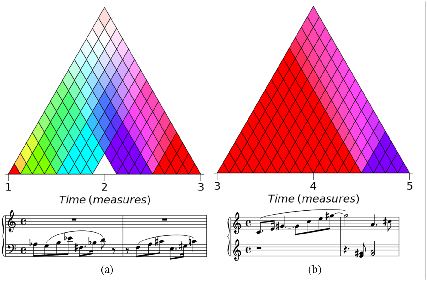
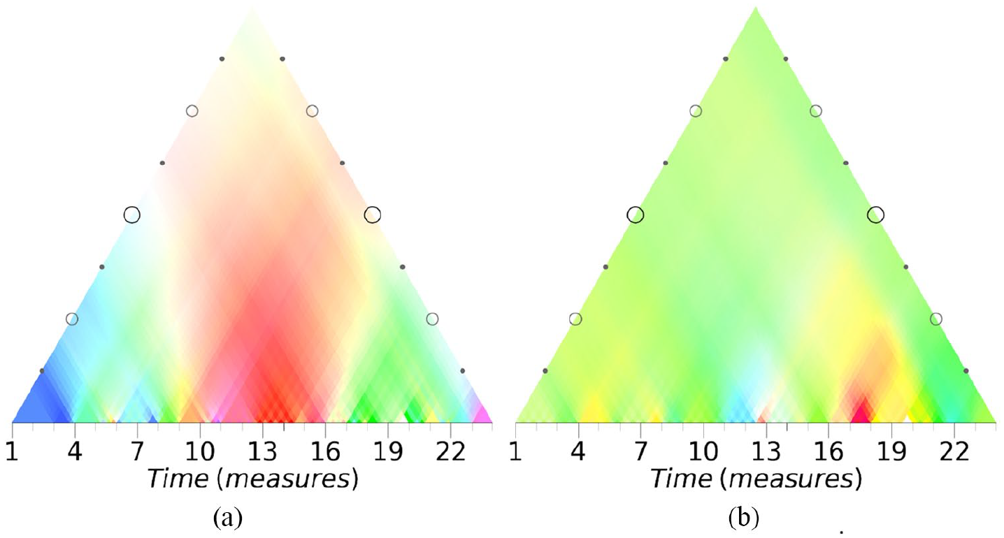
Wavescape and scores for the opening of Liszt’s Faust Symphony (S. 108), third coefficient (resolution of an eighth-note).

The first two measures are remarkable in that they use all 12 pitch classes in a very systematic fashion. With the exception of the initial A♭, the Faust motive comprises four augmented triads that together form the chromatic scale, effectively resulting in a 12-tone row. Each segment at the bottom of the wavescape shown in Figure 10a corresponds to the duration of an eighth-note. Segments that correspond to the single notes as well as to augmented triads are completely opaque since both maximize the normalized magnitudes for the third coefficient. Moreover, notes that belong to a common augmented triad are colored identically. The colors green, cyan, purple, and red correspond to D+ ( $ϕ_{3} = π$ ), D♯+ ( $ϕ_{3} = \frac{3}{2} π$ ), C+ ( $ϕ_{3} = 0$ ), and C♯+ ( $ϕ_{3} = \frac{1}{2} π$ ), respectively (see Figure 7). Bar 1 contains the augmented triads D♯+ and D+ that together form the hexatonic scale $H_{2, 3} = (0, 0, 1, 1, 0, 0, 1, 1, 0, 0, 1, 1)$ . The diamond that corresponds to bar 1 is therefore colored turquoise (see Figure 7c). Analogously, bar 2 expresses $H_{0, 1} = (1, 1, 0, 0, 1, 1, 0, 0, 1, 1, 0, 0)$ and is colored pink. Moreover, these hexatonic scales are complementary; they partition the full chromatic scale. Consequently, the leftmost diamond on third topmost row that represents the entire first two bars (except the final C) is completely white with a normalized magnitude of $0$ .⁹ Including the final C produces the light red color of the topmost diamond in Figure 10a.

Bars 3 and 4 consist almost entirely of an arpeggiation of C+, followed by C♯ + in the second half of bar 4. As before, those are reflected in the maximal opacity of the corresponding red and purple areas in the wavescape in Figure 10b. Together, these augmented triads form the hexatonic scale $H_{0, 1}$ whose phase corresponds to pink. As mentioned above, this pink hue is also the dominating color for the opening of the symphony. In contrast to the first two bars (see Figure 10a) where Liszt rotates through all augmented triads, the tonal material used in bars 3–4 presents the overall tonality of the piece (Longyear & Covington, 1986; Cohn, 2012; Argentino, 2018), so that the initial four bars of the first movement can be interpreted as establishing a hexatonic tonality, in analogy to the establishment of a key at the beginning of tonal pieces (e.g. Bach’s C-major prelude, see Figure 3 and the analysis below).

The motivic material of bars 1–11 is repeated in bars 12–22 in a transposed version. Specifically, the repetition of bars 1–2 in bars 12–13 is transposed down a major third. In bar 14, the repetition of the arpeggiated C+ from bar 3, Liszt repeats the penultimate note, which results in the transposition of the subsequent material by a major third up. The changes obtained by major-third transpositions are not visible in the wavescape for the third coefficient in Figure 9a because they remain within the same hexatonic and thus do not change the overall tonality.

However, the major-third transpositions are clearly visible through the wavescape of the first coefficient (Figure 11) that represents the chromatic circle. The main pitch classes A♭, E, and C correspond to the green, blue, and red areas, respectively, according to the color mapping in Figure 7a. The upper part of the first coefficient’s wavescape fades into white because the main pitch classes form a symmetric chord (an augmented triad) and are used similarly often in the opening bars—they cancel each other out.

Figure 11.

Wavescape for Liszt’s Faust Symphony (S. 108), first coefficient (resolution of an eighth-note).

Josquin: Motet Ave Maria (1475)

Josquin’s motet Ave Maria serves as a model for for Renaissance counterpoint.¹⁰ The time signature of this piece is 2/1 and it consists of 163 bars in modern notation; we chose a resolution of one breve (two whole-notes) for the wavescape plots of this motet. As one would expect, the tonal material in this piece is largely diatonic with some exceptions where accidentals (ficta) are used for particular cadential circumstances, for instance to strengthen leading-tone tensions.

Consequently, the fifth coefficient has the strongest average normalized magnitude ( ${\bar{α}}_{5} = . 61$ ). This indicates that the piece’s tonal material is predominantly drawn from Guido’s hexachord ( ${\bar{α}}_{5} = . 64$ ) rather than from a diatonic scale ( ${\bar{α}}_{5} = . 53$ ; see Figure 7). This value is large in comparison with the other excerpts, only rivalled by the value for the third coefficient of the Faust Symphony ( ${\bar{α}}_{3} = . 65$ ). As we have seen above, the introduction of the symphony is particularly systematic in its use of the augmented triad, reflecting early characteristics of Liszt’s “experimental idiom” (Forte, 1977, p. 209). In the case of Josquin’s motet, the relatively high average normalized magnitude indicates that it is an almost entirely diatonic composition. This, of course, is highly conventional for the Renaissance.

The overall tonal unity of the piece, its close adherence to a single diatonic scale, and the lack of modulations are immediately evident in Figure 12 as shown by the dominance of the orange color. On the lower levels of the wavescape one can see patches of red and green. While the overall key of this piece is C major, its internal cadences may refer to scale degrees other than the tonic. Moreover, cadences in the Renaissance often conclude on perfect sonorities such as octaves or fifths and not on major or minor triads as in later epochs. The bright green and red areas correspond to local cadences on E and C, respectively, where the pitch-class set consists only of a perfect fifth (E-B and C-G, see Figure 7e). The latter is particularly prominent at the end of the piece where the fifth C-G is held for six entire bars. Note that the coloring of this interval is different than the one for the C major key (see Figure 8). Anticipating what the analyses of the following pieces will show, we conclude that this piece is very homogeneous with only some minor local deviations from the key of C major that governs its overall structure.

Figure 12.

Wavescape for Josquin’s Ave Maria (c. 1484), fifth coefficient (resolution of a whole-note).

Bach: Prelude in C major BWV 846 (1722)

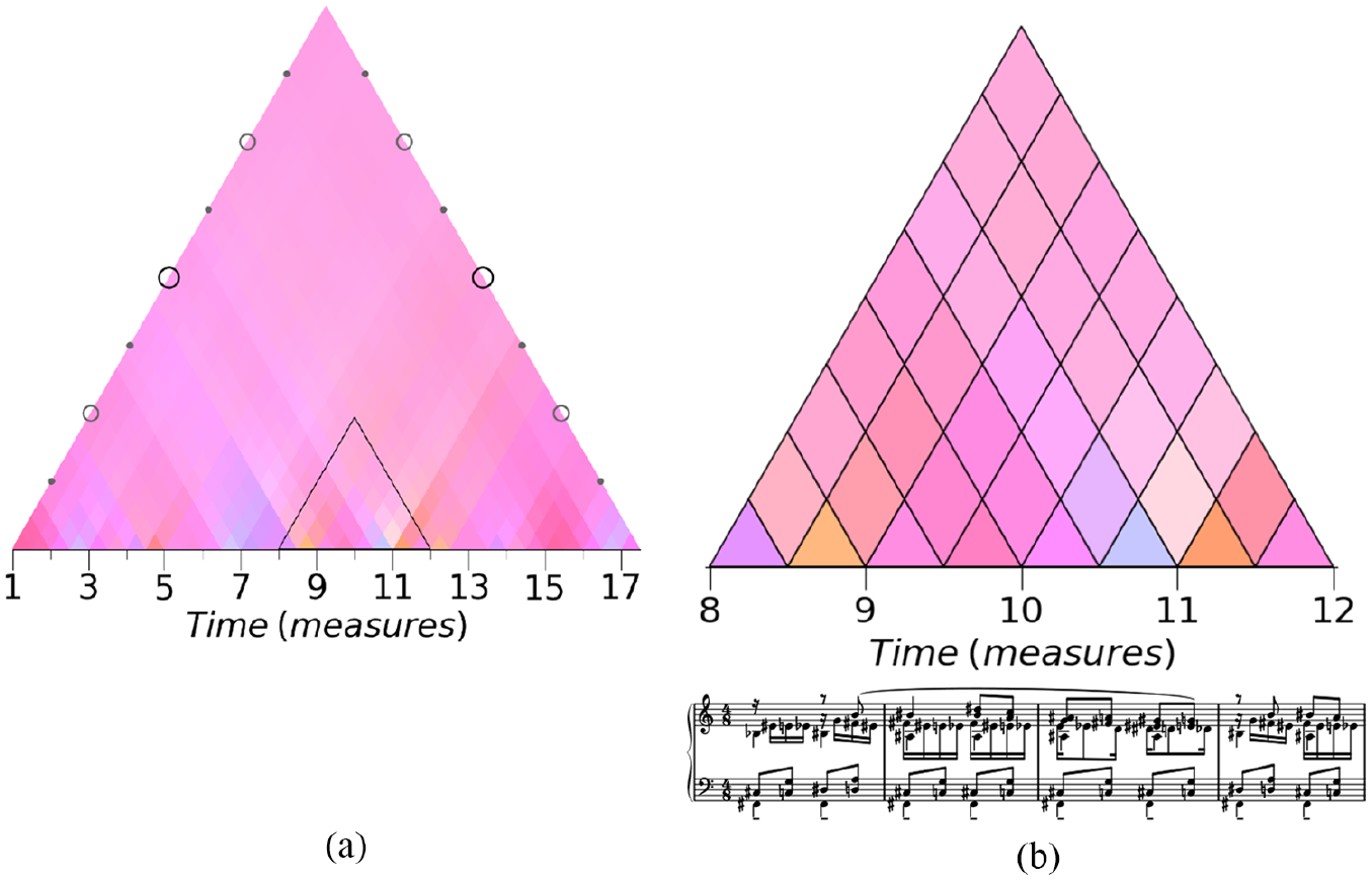
Bach’s Prelude in C major from the Well-Tempered Clavier I (1722) is a popular piece for analysis (e.g., Schenker, 1933).¹¹ Its time signature is 4/4 and it consists of 35 bars. We focus our analysis on the fifth coefficient using a resolution of one quarter-note. This coefficient has highest average normalized magnitude ( ${\bar{α}}_{5} = . 533$ , see also Table 1) because the prelude is a largely diatonic piece. Figure 13a shows the wavescape for the fifth coefficient of the prelude; it resembles that of Josquin’s Ave Maria, in particular on the higher levels colored in bright orange.

Figure 13.

Wavescape for Bach’s Prelude in C major Prelude (BWV 846), fifth, third, fourth and first coefficient (resolution of a quarter-note).

However, the harmonic structure of the two pieces differs in several details, which become apparent upon a closer look at the more local levels of the wavescapes. The initial four bars of the prelude consist of a cadence in C major, thus establishing its main key, which is then prolonged in the following bars until another cadence in the tonic key in bar 19. The corresponding section of the wavescape in Figure 13a displays a yellow sub-triangle, visualizing the key of C major with some green parts which stand for dominant chords or tonicizations of G major (see Figure 7e). The overall color of this section is yellow or a very bright orange, as one would expect from a Baroque piece in C major. Subsequently, the piece shifts to the plagal side of C (towards F) in bars 20–21, shown in bright red. A similar shift appears again shortly before the end of the piece in bars 32–33 before the final cadence on the global tonic. An other interesting detail is that the wavescape distinguishes between the modulation to G major in bars 5–11 (shown in yellow-green) and the extended dominant in bars 24–31 (shown in orange-red), caused by the presence of F $#$ and F natural, respectively.

The wavescapes for the third and fourth coefficients (Figures 13b and 13c, respectively) provide further analytical insights about the local harmonic structure of the prelude. Even though the global opacity of the colors is generally lower than in the fifth coefficient, the lower levels have very high opacities. This indicates that almost each bar in the piece contains a triad or a seventh chord (see Figure 6). Moreover, these two wavescapes show much more frequent phase changes, reflecting the fast harmonic rhythm (change of harmony every bar, applied dominants, etc.).

The pedal point on G in bars 24–31 leads in the third coefficient to a large greenish region towards the end of the piece. In accordance with Schenkerian theory (Cadwallader & Gagné, 1998), this represents the harmonic function of a prolonged dominant of the chords involved. Whereas this region was not prominent in the fifth coefficient because the G7 chord is part of the main key of the piece, it does stand out in the third coefficient because here we observe local changes between triads.

A final insight into the harmonic structure of this piece can be drawn from the wavescapes of the first coefficient. It shows a smooth color transition from pink in bar 1 to dark blue in bar 16 (see Figure 13d), encompassing all the colors on the spectrum between these two poles in a counter-clockwise phase change (see Figure 7a). This transition is mainly caused by the diatonically descending line in the bass and tenor (left hand). The pattern is broken in bars 9–10 and 17–18 where G major and C major are approached by two falling fifths to strengthen the cadential arrivals on the dominant and the tonic, respectively.

Chopin’s Prelude in A minor op. 28 no. 2

Chopin’s Prelude op. 28 no. 2 is an unusual piece. With only 23 bars in a 4/4 time signature, it is one of the shortest of Chopin’s preludes.¹² Its key signature is A minor but the tonality of the piece is notoriously difficult to determine (Hoyt, 1985). For the visualization in the wavescapes we chose a resolution of one quarter-note. The wavescapes with the highest normalized magnitudes for the Prelude are the fourth ( ${\bar{α}}_{4} = . 329$ ) and the fifth ( ${\bar{α}}_{5} = . 451$ ) coefficients.

The fourth coefficient (Figure 14a) displays few colors with strong opacity which are, from left to right, blue, green-cyan, red, green, and finally pink. These hues indicate the diminished seventh chords or octatonic scales that the respective segments resemble most closely (see Figure 7). For example, the blue area in bars 1–3 is an E minor chord plus an A♯that can also be seen as a diminished triad on E plus B. The segment in bars 4–8 is more heterogeneous on the local level but on higher levels groups to a green-cyan part of the wavescape, indicating that the diminished chord on D is salient in this region. The subsequent red section from bar 9 to bar 15 is largely governed by pitch classes from the diminished chord C-D♯-F♯-A. This chord never occurs in its entirety in this section but only in parts, and the wavescape reveals how its member notes tie the segment together in bars 9–15, even though they are never present at the same time. This diminished chord thus lies at a structurally higher level than the surface of the music. The following green region in bars 17–22 is relatively strong, which indicates that the pitch classes F, D and B occur relatively frequently. The A minor chord that concludes the piece in bar 23 is shown in pink.

Figure 14.

Wavescape for Chopin’s Prelude in A minor op. 28 no. 2, fourth and fifth coefficient (resolution of a quarter-note).

The wavescape for the fourth coefficient shows the existence of a mirror axis around the the center of the piece (only approximately, since the pink parts of the end do not mirror the blue parts of the beginning). This symmetry is easy to overlook in a traditional analysis of the score since it is somewhat disguised by different textures. Because wavescapes only consider the tonal content, they abstract from the concrete realizations of the musical material and are able to capture more general relations.

The fifth coefficient shown in Figure 14b displays mainly green and yellow colors. This indicates the use of notes predominantly from the keys of A minor and E minor (see Figure 8). Bar 17 stands out with its bright red color. The melodic line in this bar contains the pitch classes F, A, C and G, which form an F major triad (plus ninth) that is not part of the E minor scale. This segment thus deviates strongly from the overall green color. The deviation marks an important point in the piece, which is further supported by a change of texture to a monophonic line in the right hand.

As mentioned before, the prelude is known for being ambiguous in terms of its key. While its key signature indicates A minor, its first bars appear to be in E minor, the right-hand melody does not emphasize a tonal center clearly, and triadic harmonies are perturbed by chromatic neighbor notes (except in the final bars of the piece). However, the relatively homogeneous color of the wavescape for the fifth coefficient indicates that the pitch-class content of A minor is used on multiple levels in the prelude. This supports the view that the piece can be regarded, overall, as being in A minor.

Scriabin’s Prelude op. 74 no. 2

Scriabin’s Prelude op. 74 no. 2 for piano (Très lent, contemplatif)¹³ was written in 1914, shortly before the composer’s death. Its time signature is 4/8 and it consists of 17 bars. For the visualization in the wavescapes, we chose a resolution of one quarter-note. Overall, this short piece has a homogeneous tonality and largely features unconventional harmonies and melodic lines. Both aspects are expressed in the particular color patterns of the corresponding wavescapes that reveal many details of the tonal structure of the piece. The largest average normalized magnitudes is ${\bar{α}}_{4} = . 375$ (see Table 1 in the Appendix). Visually, this corresponds to the high opacity of the fourth coefficient’s wavescape shown in Figure 15a.

Figure 15.

Wavescape for Scriabin’s Prelude op. 74 no. 2, fourth coefficient (resolution of a quarter-note).

The high magnitude ${\bar{α}}_{4}$ suggests that diminished seventh chords and octatonic scales are of high relevance for the tonal structure of the piece. The score of the prelude shows that, indeed, the piece is governed by an overarching octatonic scale, namely $O_{0, 1} = (1, 1, 0, 1, 1, 0, 1, 1, 0, 1, 1, 0)$ . The fact that the wavescape of the fourth coefficient is relatively homogeneous both in hue and opacity confirms that an octatonic scale governs this piece on virtually all hierarchical levels. The dominant pink color in this wavescape corresponds exactly to the mentioned octatonic scale, as can be seen in Figure 7d. Additionally, there are four pitch classes that are not part of the octatonic scale $O_{0, 1}$ , namely B, D, F and G♯, all of which do eventually occur in the piece. Those pitch classes form a fully diminished triad ${D \circ}^{7}$ that is exactly opposite to $O_{0, 1}$ according to the fourth coefficient, as shown in Figure 7d.

One might be misled by the almost uniform character of the piece to overlook some of the more intricate harmonic aspects that become apparent upon a closer look at the wavescape. Figure 15b shows the wavescape for bars 8–11 of Scriabin’s prelude. The members of the D diminished-seventh chord appear in those bars, but the wavescape of the section does not contain any shades of green—the color of Dº⁷ for the fourth coefficient (see Figure 7d). Instead, some triangles are colored in shades of purple and orange. A close reading of the pitch-class content of bars 10 and 11 explains the absence of a green hue despite the presence of out-of-scale pitch classes. The second half of bar 10 contains G♯, E♯and D, thus all members of Dº⁷ except B, whereas the first half of bar 11 contains B, E♯ and D, thus all members of the fully diminished chord except G♯. The members of the diminished chord pull the color from the octatonic pink in the green direction towards the white center (see Figure 7d). The absence of pitch classes B and G♯corresponds to a slightly leftward (in the blue direction, resulting in a purple hue) and rightward (in the red direction, resulting in an orange hue) direction, respectively.

While this piece is locally volatile and features chromatic passing notes and fluctuations between the octatonic scale and its complementary diminished seventh chord, its overall tonal stability is remarkable and clearly expressed by the homogeneous color of the wavescape for the fourth coefficient.

Coltrane’s Giant Steps

The next case study focuses on the jazz tune Giant Steps by John Coltrane.¹⁴ The time signature is 4/4 and one chorus consists of 16 bars. For the visualization of the wavescapes, a resolution of one quarter-note was chosen. Similarly to the Faust Symphony, the wavescape standing out the most is the one of the third coefficient with an average normalized magnitude of ${\bar{α}}_{3} = . 333$ . The second strongest is the fifth coefficient with ${\bar{α}}_{5} = . 215$ . We therefore concentrate our analysis on those two wavescapes.

The harmonic structure of the piece is very regular. It consists of ii-V-I progressions in the keys of G, E♭ and B which are related by major thirds, to which the title of the piece might allude (Weiskopf & Ricker, 1991; Goodheart, 2001). Since each ii-V-I progression establishes a local key, the PCVs representing those progressions each have a homogeneous but distinct coloring for the fifth coefficient. They are clearly visible as regularly alternating green, purple and blue areas on the lower levels of Figure 16a.

Figure 16.

Wavescape for Coltrane’s Giant Steps, fifth and third coefficient (resolution of a quarter-note).

The almost uniform coloring of the wavescape for the third coefficient shown in Figure 16b is remarkable. The tonics of the local keys form an augmented triad—the prototype of the third coefficient—which explains the large average magnitude ${\bar{α}}_{3}$ . The augmented triad E♭-G-B corresponds to the mint color (see Figure 7c) and the wavescape elegantly visualizes the extent to which this triad is characteristic of the piece.

Webern and Ligeti

We now investigate whether the wavescape visualizations are useful for the analysis of 20^th-century post-tonal music. Specifically, we compare the wavescapes of Webern’s serial composition Variations for Piano op. 27 no. 1 (Sehr mäßig),¹⁵ and Ligeti’s Études pour Piano no. 2 (Cordes à vide).¹⁶

Webern’s piece has a time signature of 3/16 with 54 bars in total and we chose a resolution of one 16th note. For Ligeti’s piece, which has no written time signature but contains 39 bars of a 4/4 duration,¹⁷ we chose a resolution of one quarter-note.

The purpose of the 12-tone technique, employed in Webern’s Variations, is to avoid establishing a key or any sense of key. In the words of Schoenberg, “[a] style based on this premise treats dissonances like consonances and renounces a tonal center” (Schoenberg, 1950, p. 105). This compositional technique defines the succession of all 12 pitch classes a priori without any further tonal considerations such as consonance, dissonance, or stacked thirds (Covach, 2002; Wason, 1987). Consequently, the average normalized magnitude for the fifth coefficient is very small ( ${\bar{α}}_{5} = . 046$ ) and indeed minimal among all the coefficients for this piece (see Table 1).

Since each 12-tone row consists of all chromatic pitch classes, their corresponding color is almost white (not entirely due to varying note durations). This also affects the overall opacity of all wavescapes for this piece; the largest average normalized magnitude is ${\bar{α}}_{2} = . 080$ and the smallest is ${\bar{α}}_{5} = . 046$ (shown in Figure 17 for comparison with Ligeti). Only on a very local level can one observe larger magnitudes, caused by consonant co-occurrences of certain pitch-classes. The colored patches at the lower levels of this composition do not extend to larger time spans because their tonal material is not diatonic (in contrast to previous analyses of the fifth coefficient). The keyscape analyses of this piece by Sapp (2001, 2005) also show a lack of structure. Our approach generalizes this finding by showing that the piece does not lead to high magnitudes for any of the Fourier coefficients.

Figure 17.

Wavescape for Webern’s Variations for Piano, fifth coefficient (resolution of a 16th note).

The wavescapes for Ligeti’s étude look very similar at first sight (compare Figures 26 and 25 in the Appendix). All wavescapes are rather faded out due to overall small average normalized magnitudes (largest: ${\bar{α}}_{5} = . 105$ , smallest: ${\bar{α}}_{6} = . 037$ ). This is somewhat surprising since the étude largely consists of chains of perfect fifths (Polth, 2016) that should give rise to high magnitudes in the fifth coefficient. For example, the first group of notes in the right hand is A-D-G-D-A-D, and the first one in the left hand is C-F-E♭-B♭. Although the union of these two chains would fit perfectly into the diatonic scale of B♭ major, longer chains as well as the superposition of several chains introduce chromatic steps that obfuscate the underlying organization by fifths. The only exception occurs in the final two bars (37–38), where the left hand plays alone and the magnitudes are very high (see Figure 18) because they contain only the notes B♭-F-E-A. These notes span the F major diatonic scale B♭-F-C-G-D-E-A. Since G is in its center, the hue of the wavescape in these two bars corresponds to the hue for G (see Figure 7e).

Figure 18.

Wavescape for Ligeti’s Études pour Piano no. 2, fifth coefficient (resolution of a quarter-note).

A limitation of the present approach is caused by the vertical partitioning of the pieces into contiguous segments in time, which fragments horizontal structures such as the chains of fifths in Ligeti’s étude and the 12-tone rows in Webern’s variation. However, because chains of fifths generally have high magnitudes in the fifth coefficient (see Figure 7e), the respective wavescape shows a succession of colors that loosely corresponds to the structure of the étude (see also the wavescape of the first coefficient, shown in Figure 25 in the Appendix). In contrast, Webern’s 12-tone rows cause lower magnitudes already on low levels of the fifth coefficient (shown in Figure 17). Furthermore, none of the coefficients for Webern’s variation exhibit high magnitudes because of the equal usage of all twelve pitch classes in this piece. If it were additionally the case that, for some segments, each pitch class would also have the same duration, the corresponding parts of the wavescape would be perfectly white. We expect other serial compositions to have similarly transparent and colorful wavescapes. More insightful analyses thus require additional tools such as set theory or voice-leading analysis (e.g., Straus, 2005).

Discussion

As the case studies have demonstrated, wavescapes extend the methodological toolkit of music analysis in several ways. They combine the hierarchical representation of a piece of music (such as in keyscapes) with the insights obtained from the application of the DFT to pitch-class sets. Since the DFT maps pitch-class sets to a continuous color space, wavescape plots are more fine-grained than keyscapes based on templates that rely on categorical labels. Wavescapes offer a new methodology for analyzing the tonality of a piece without relying on predefined templates (such as major/minor key profiles) and thus expand the application also to extended tonal styles. As such, they do not rely on relatively narrow music-theoretical concepts that are most appropriate only for the common-practice era (such as “key”) but offer a more general approach to the tonality of pieces through the different Fourier coefficients.

However, the wavescape methodology is somewhat limited in the scope of its possible applications. For example, it might not provide many insights into atonal works or musical styles that are based on musical properties other than pitch, for instance rhythm or timbre. Furthermore, the quality and thus the interpretability of wavescapes relies on an accurate representation of the pitch-class content of a piece which can either be extracted directly from a symbolic encoding or inferred from audio data. Whether one considers note durations or counts can also influence the wavescapes considerably.

A quantitative comparison of multiple wavescapes—either of different coefficients for the same piece or of the same coefficient for different pieces—might also be challenging. While wavescapes are derived deterministically from their pitch-class input, they are difficult to interpret on their own, and one is often required to consult the score or a recording of the piece. Moreover, the DFT requires a circular representation such as pitch classes for its input. This entails the assumption of octave and enharmonic equivalence, which might be a serious limitation for some music-analytical aims.

However, the fact that the DFT is applied to circular data enables the potential application of wavescapes to other domains, in particular meter and rhythm where circular representations are commonplace (Milne et al., 2015, 2017). The perceptual relevance of the DFT for rhythms has been demonstrated by Milne and Herff (2020) and it is promising to apply the DFT in psychological studies in the domain of pitch. The cognitive relevance of the DFT in this domain is plausible because it separates the transpositionally invariant structure of chords and scales form their realization in absolute pitches.

One can also conceive of further benefits of wavescapes apart from visualization. The colors of the segments in a wavescape provide numerical values for the phases and magnitudes of the involved pitch-class sets from which a number of statistics can be derived (see e.g., Table 1 in the Appendix for the average normalized magnitudes). This can constitute a basis for large-scale corpus studies and applications of more rigorous statistical methods, for example to compare composers and historical periods (for a related approach based on interval classes, see Weiß et al., 2019, and Harasim et al., 2021).

Another possible adaptation could be applications to music that are based on tuning systems other than 12-tone equal temperament or that divide the octave by numbers other than 12. This would result in new prototypes for the coefficients, as they would represent new even chords in those tuning systems and might provide novel insights into non-Western musical styles.

Conclusion

This article presented a novel visualization method for hierarchical music analysis using the discrete Fourier transform (DFT) called wavescapes. Wavescapes permit the relevance of particular tonal structures in pieces of music to be observed easily at several hierarchical levels. This bottom-up approach augments and complements detailed analyses of a score. With the added knowledge of the interpretations of the respective Fourier coefficients, the tonality of a composition can be understood by comparing the wavescapes for the different coefficients. In particular, it is possible to disentangle complementary aspects of a piece by considering several wavescapes. Since the DFT is a deterministic mapping from pitch-class content into Fourier space, it provides an objective summary of the piece. However, music-theoretical expertise is still required for analysis and interpretation. Finally, we provide a free open-source visualization library that enables this method to be used easily, for example by music theorists in their own research or students in the classroom.

Footnotes

Appendix

Table 1.

Average normalized magnitudes ${\bar{α}}_{k}$ (± standard deviations) for Fourier coefficients $k = 1, \dots, 6$ and all analyzed examples.

$k$	1	2	3	4	5	6
Liszt	$. 179 (\pm . 031)$	$. 157 (\pm . 028)$	$. 652 (\pm . 014)$	$. 188 (\pm . 022)$	$. 163 (\pm . 021)$	$. 172 (\pm . 047)$
Josquin	$. 127 (\pm . 012)$	$. 272 (\pm . 006)$	$. 322 (\pm . 009)$	$. 117 (\pm . 012)$	$. 611 (\pm . 002)$	$. 094 (\pm . 014)$
Bach	$. 228 (\pm . 018)$	$. 245 (\pm . 017)$	$. 252 (\pm . 023)$	$. 191 (\pm . 023)$	$. 533 (\pm . 009)$	$. 138 (\pm . 023)$
Chopin	$. 098 (\pm . 015)$	$. 224 (\pm . 013)$	$. 309 (\pm . 023)$	$. 329 (\pm . 028)$	$. 451 (\pm . 013)$	$. 175 (\pm . 016)$
Scriabin	$. 093 (\pm . 003)$	$. 302 (\pm . 014)$	$. 234 (\pm . 007)$	$. 375 (\pm . 003)$	$. 120 (\pm . 018)$	$. 220 (\pm . 006)$
Coltrane	$. 081 (\pm . 004)$	$. 097 (\pm . 009)$	$. 333 (\pm . 006)$	$. 088 (\pm . 005)$	$. 215 (\pm . 028)$	$. 151 (\pm . 009)$
Ligeti	$. 055 (\pm . 004)$	$. 078 (\pm . 008)$	$. 062 (\pm . 007)$	$. 053 (\pm . 004)$	$. 105 (\pm . 015)$	$. 037 (\pm . 003)$
Webern	$. 082 (\pm . 014)$	$. 092 (\pm . 020)$	$. 068 (\pm . 010)$	$. 068 (\pm . 013)$	$. 056 (\pm . 009)$	$. 078 (\pm . 013)$

Acknowledgements

The authors thank Christoph Finkensiep, Johannes Hentschel, Steffen Herff, Robert Lieck and Andrew McLeod, as well as Thomas Noll and Jason Yust for their support and valuable feedback. We also thank the editor Jane Ginsborg and two anonymous reviewers for their helpful comments and suggestions.

Declaration of conflicting interests

The authors declared no potential conflicts of interest with respect to the research, authorship, and/or publication of this article.

Funding

The authors disclosed receipt of the following financial support for the research, authorship, and/or publication of this article: This project has received partial funding from the European Research Council (ERC) under the European Union’s Horizon 2020 research and innovation program under grant agreement no. 760081-PMSB. It was also partially funded through the Swiss National Science Foundation (SNF) within the project “Distant Listening – The Development of Harmony over Three Centuries (1700–2000)” (grant no. 182811). The authors thank Claude Latour for supporting this research through the Latour Chair in Digital Musicology at EPFL.

ORCID iDs

Cédric Viaccoz

Fabian C. Moss

Notes

References

Abdallah

Gold

Marsden

(2016). Analysing symbolic music with probabilistic grammars. In Meredith

(Ed.), Computational music analysis (pp. 157–189). Springer.

Albrecht

Shanahan

(2013). The use of large corpora to train a new type of key-finding algorithm: An improved treatment of the minor mode. Music Perception: An Interdisciplinary Journal, 31(1), 59–67. https://doi.org/10.1525/mp.2013.31.1.59

Aldwell

Schachter

Cadwallader

(2010). Harmony and voice leading (4th ed.). Cengage Learning.

Amiot

(2007). David Lewin and maximally even sets. Journal of Mathematics and Music, 1(3), 1–21. https://doi.org/10.1080/17459730701654990

Amiot

(2016). Music through Fourier space: Discrete Fourier transform in music theory. Springer International Publishing AG.

Amiot

(2020). Entropy of Fourier coefficients of periodic musical objects. Journal of Mathematics and Music. https://doi.org/10.1080/17459737.2020.1777592

Arbib

M. A.

(Ed.). (2013). Language, music, and the brain: A mysterious relationship. MIT Press.

Argentino

(2018). Schoenberg and Liszt: Hexatonic collections across the great tonal divide. Music Analysis, 37(2), 184–202. https://doi.org/10.1111/musa.12093

Bribitzer-Stull

(2006). The Ab-C-E complex: The origin and function of chromatic major third collections in nineteenth-century music. Music Theory Spectrum, 28(2), 167–190. https://doi.org/10.1525/mts.2006.28.2.167

10.

Cadwallader

Gagné

(1998). Analysis of tonal music: A Schenkerian approach. Oxford University Press.

11.

Caplin

W. E.

(1998). Classical form: A theory of formal functions for the instrumental music of Haydn, Mozart and Beethoven. Oxford University Press.

12.

Clough

Douthett

(1991). Maximally even sets. Journal of Music Theory, 35(1), 93–173. https://doi.org/10.2307/843811

13.

Cohn

(1996). Maximally smooth cycles, hexatonic systems, and the analysis of late-romantic triadic progressions. Music Analysis, 15(1), 9–40. https://doi.org/10.2307/854168

14.

Cohn

(2012). Audacious euphony: Chromatic harmony and the triad’s second nature. Oxford University Press.

15.

Covach

(2002). Twelve-tone theory. In Christensen

(Ed.), The Cambridge history of Western music theory (pp. 603–627). Cambridge University Press.

16.

Forte

(1977). The structure of atonal music. Yale University Press.

17.

Gárdonyi

Nordhoff

(2002). Harmonik. Möseler Verlag.

18.

Gilbert

Conklin

(2007). A probabilistic context-free grammar for melodic reduction. In Proceedings of the 20th International Workshop on Artificial Intelligence and Music (pp. 83–94).

19.

Goodheart

(2001). The “Giant Steps” fragment. Perspectives of New Music, 39(2), 63–95. https://www.jstor.org/stable/833564

20.

Granroth-Wilding

Steedman

(2012). Statistical parsing for harmonic analysis of jazz chord sequences. In Proceedings of the International Computer Music Conference (pp. 478–485).

21.

Haas

(2004). Die neue Tonalität von Schubert bis Webern: Hören und Analysieren nach Albert Simon. Florian Noetzel.

22.

Harasim

(2020). The learnability of the grammar of jazz: Bayesian inference of hierarchical structures in harmony. [Doctoral dissertation, École polytechnique fédérale de Lausanne]. EPFL scientific publications. http://doi.org/10.5075/epfl-thesis-10404

23.

Harasim

Moss

F. C.

Ramirez

Rohrmeier

(2021). Exploring the foundations of tonality: Statistical cognitive modeling of modes in the history of Western classical music. Humanities and Social Sciences Communications, 8(5), 1–11. https://doi.org/10.1080/17459737.2019.1696899

24.

Harasim

O’Donnell

T. J.

Rohrmeier

(2019). Harmonic syntax in time: Rhythm improves grammatical models of harmony. In Flexer

Peeters

Urbano

Volk

(Eds.), Proceedings of the 20th International Society for Music Information Retrieval Conference (pp. 335–342). https://doi.org/10.5281/zenodo.3527812

25.

Harasim

Rohrmeier

O’Donnell

T. J.

(2018). A generalized parsing framework for generative models of harmonic syntax. In Gómez

Humphrey

Benetos

(Eds.), Proceedings of the 19th International Society for Music Information Retrieval Conference (pp. 152–159). https://doi.org/10.5281/zenodo.1492367

26.

Harasim

Schmidt

S. E.

Rohrmeier

(2020). Axiomatic scale theory. Journal of Mathematics and Music, 14(3), 223–244. https://doi.org/10.1080/17459737.2019.1696899

27.

Harding

J. D.

(2020). Computer-aided analysis across the tonal divide: Cross-stylistic applications of the discrete Fourier transform. In De Luca

Flanders

(Eds.), Proceedings of the Music Encoding Conference (pp. 95–104). http://doi.org/10.17613/2n0b-1v04

28.

Hoffman

(2008). On pitch-class set cartography: Relations between voice-leading spaces and Fourier spaces. Journal of Music Theory, 52(2), 219–249. https://doi.org/10.1215/00222909-2009-016

29.

Honingh

Bod

(2010). Pitch class set categories as analysis tools for degrees of tonality. In Downie

J. S.

Veltkamp

R. C.

(Eds.), Proceedings of the 11th International Society for Music Information Retrieval Conference (pp. 459–464). https://doi.org/10.5281/zenodo.1417533

30.

Honingh

Bod

(2011). Clustering and classification of music by interval categories. In Agon

Andreatta

Assayag

Amiot

Bresson

Mandereau

(Eds.), Mathematics and computation in music: Lecture notes in computer science (pp. 346–349). Springer. https://doi.org/10.1007/978-3-642-21590-2_30

31.

Horton

(2018). Form and orbital tonality in the finale of Bruckner’s seventh symphony. Music Analysis, 37(3), 271–309. https://doi.org/10.1111/musa.12124

32.

Hoyt

R. J.

(1985). Chopin’s prelude in A minor revisited: The issue of tonality. Theory Only, 8(6), 7–16.

33.

Katz

(2017). Harmonic syntax of the twelve-bar blues form. Music Perception: An Interdisciplinary Journal, 35(2), 165–192. https://doi.org/10.1525/mp.2017.35.2.165

34.

Keiler

(1978). Bernstein’s “The unanswered question” and the problem of musical competence. Musical Quarterly, 62(2), 195–222.

35.

Kirlin

P. B.

Jensen

D. D.

(2011). Probabilistic modeling of hierarchical music analysis. In Klapuri

Leider

(Eds.), Proceedings of the 12th International Society for Music Information Retrieval Conference (pp. 393–398). https://doi.org/10.5281/zenodo.1417119

36.

Kopp

(2002). Chromatic transformations in nineteenth-century music. Cambridge University Press.

37.

Krumhansl

C. L.

(1990). Cognitive foundations of musical pitch. Oxford University Press.

38.

Lendvai

(1971). Béla Bartók: An analysis of his music. Kahn & Averill.

39.

Lerdahl

(2001). Tonal pitch space. Oxford University Press.

40.

Lerdahl

Jackendoff

R. S.

(1983). A generative theory of tonal music. MIT Press.

41.

Lewin

(1959). Re: Intervallic relations between two collections of notes. Journal of Music Theory, 3(2), 298–301. https://doi.org/10.2307/842856

42.

Lewin

(2001). Special cases of the interval function between pitch-class sets X and Y. Journal of Music Theory, 45(1), 1–29. https://doi.org/10.2307/3090647

43.

Lieck

Rohrmeier

(2020). Modelling hierarchical key structure with pitch scapes. In Cumming

Lee

J. H.

McFee

Schedl

Devaney

McKay

Zangerle

de Reuse

(Eds.), Proceedings of the 21th International Society for Music Information Retrieval Conference (pp. 811–818). https://doi.org/10.5281/zenodo.4245558

44.

Lieck

Moss

F. C.

Rohrmeier

(2020). The tonal diffusion model. Transactions of the International Society for Music Information Retrieval, 3(1), 153–164. https://doi.org/10.5334/tismir.46

45.

Longyear

R. M.

Covington

K. R.

(1986). Tonal and harmonic structures in Liszt’s Faust symphony. Studia Musicologica Academiae Scientiarum Hungaricae, 28(1), 153–171.

46.

Manning

Schütze

(2003). Foundations of statistical natural language processing (6th ed.). MIT Press.

47.

Marr

(1982). Vision: A computational investigation into the human representation and processing of visual information. W. H. Freeman and Company.

48.

Mavromatis

(2012). Exploring the rhythm of the Palestrina style: A case study in probabilistic grammar induction. Journal of Music Theory, 56(2), 169–223. https://doi.org/10.1215/00222909-1650406

49.

Messiaen

(1944). Technique de mon langage musical. Alphonse Leduc.

50.

Milne

A. J.

Herff

S. A.

(2020). The perceptual relevance of balance, evenness, and entropy in musical rhythms. Cognition, 203, Article 104233. https://doi.org/10.1016/j.cognition.2020.104233

51.

Milne

A. J.

Bulger

Herff

S. A.

(2017). Exploring the space of perfectly balanced rhythms and scales. Journal of Mathematics and Music, 11(2–3), 101–133. https://doi.org/10.1080/17459737.2017.1395915

52.

Milne

A. J.

Bulger

Herff

S. A.

Sethares

W. A.

(2015). Perfect balance: A novel principle for the construction of musical scales and meters. In Collins

Meredith

Volk

(Eds.), International Conference on Mathematics and Computation in Music (pp. 97–108). Springer. https://doi.org/10.1007/978-3-319-20603-5_9

53.

Noll

(2019). Insiders’ choice: Studying pitch class sets through their discrete Fourier transformations. In Montiel

Gomez-Martin

Agustín-Aquino

O. A.

(Eds.), Mathematics and computation in music (pp. 371–378). Springer International Publishing. https://doi.org/10.1007/978-3-030-21392-3_32

54.

Ong

Khoo

H. K.

(2014). Generalization of hue in the RGB cube space. In Baozong

Qiuqi

Xiaofang

(Eds.), Proceedings of the 12th International Conference on Signal Processing Proceedings (pp. 631–636). https://doi.org/10.1109/ICOSP.2014.7015080

55.

Park

Kwon

Lee

Kim

Nam

(2019). A cross-scape plot representation for visualizing symbolic melodic similarity. In Flexer

Peeters

Urbano

Volk

(Eds.), Proceedings of the 20th International Society for Music Information Retrieval Conference (pp. 423–430). https://doi.org/10.5281/zenodo.3527834

56.

Polth

(2016). Nicht tonal und nicht atonal: Zur Bedeutung der Quinten in Ligetis Etüde Nr. 8 “Fém.” Studia Musicologica, 57(1–2), 121–138. https://doi.org/10.1556/6.2016.57.1-2.9

57.

Polth

(2018). The individual tone and musical context in Albert Simon’s Tonfeldtheorie. Music Theory Online, 24(4). https://doi.org/10.30535/mto.24.4.15

58.

Quinn

(2006). General equal-tempered harmony: Introduction and part I. Perspectives of New Music, 44(2), 114–158. https://www.jstor.org/stable/25164630

59.

Quinn

(2007). General equal-tempered harmony: Parts 2 and 3. Perspectives of New Music, 45(1), 4–63. https://www.jstor.org/stable/25164642

60.

Rebuschat

Rohrmeier

Hawkins

J. A.

Cross

(Eds.). (2012). Language and music as cognitive systems. Oxford University Press.

61.

Reisenweaver

A. J.

(2013). Guido of Arezzo and his influence on music learning. Music and Worship, 3(1), 37–59. http://doi.org/10.15385/jmo.2012.3.1.4

62.

Rohrmeier

(2020). The syntax of jazz harmony: Diatonic tonality, phrase structure, and form. Music Theory and Analysis, 7(1), 1–63.

63.

Rohrmeier

(2011). Towards a generative syntax of tonal harmony. Journal of Mathematics and Music, 5(1), 35–53. https://doi.org/10.1080/17459737.2011.573676

64.

Rohrmeier

Neuwirth

(2015). Towards a syntax of the classical cadence. In Neuwirth

Bergé

(Eds.), What is a cadence? (pp. 285–336). Leuven University Press.

65.

Sapp

C. S.

(2001). Harmonic visualizations of tonal music. In Proceedings of the International Computer Music Conference (pp. 423–430).

66.

Sapp

C. S.

(2005). Visual hierarchical key analysis. Computers in Entertainment, 3(4). https://doi.org/10.1145/1095534.1095544

67.

Sapp

C. S.

(2007). Comparative analysis of multiple musical performances. In Proceedings of the 8th International Conference on Music Information Retrieval (pp. 497–500). https://doi.org/10.5281/zenodo.1417693

68.

Schenker

(1933). Five graphic music analyses (Fünf Urlinie-Tafeln). Dover Books on Music Series. Dover Publications.

69.

Schoenberg

(1950). Style and idea. Philosophical Library.

70.

Schoenberg

(1969). Structural functions of harmony. Faber and Faber.

71.

Segnini

Sapp

(2005). Scoregram: Displaying gross timbre information from a score. In Kronland-Martinet

Voinier

Ystad

(Eds.), Proceedings of Computer Music Modeling and Retrieval (pp. 54–59). https://doi.org/10.1007/11751069_5

72.

Steedman

(1984). A generative grammar for jazz chord sequences. Music Perception: An Interdisciplinary Journal, 2(1), 52–77. https://doi.org/10.2307/40285282

73.

Steedman

(1996). The blues and the abstract truth: Music and mental models. In Garnham

Oakhill

(Eds.), Mental models in cognitive science: Essays in honour of Phil Johnson-Laird (pp. 305–318). Psychology Press.

74.

Straus

J. N.

(2005). Introduction to post-tonal theory (3rd ed.). Pearson Prentice Hall.

75.

Temperley

(1999). What’s key for key? The Krumhansl-Schmuckler key-finding algorithm reconsidered. Music Perception, 17(1), 65–100. https://doi.org/10.2307/40285812

76.

Tresize

(Ed.) (2017). The Cambridge companion to Debussy. Cambridge University Press.

77.

Tymoczko

(2003). Root motion, function, scale-degree: A grammar for elementary tonal harmony. Musurgia. Analyse et Pratique Musicales, X(3–4), 35–64.

78.

Tymoczko

(2008). Set-class similarity, voice leading, and the Fourier transform. Journal of Music Theory, 52(2), 251–272. https://doi.org/10.1215/00222909-2009-017

79.

Tymoczko

Yust

(2019). Fourier phase and pitch-class sum. In Montiel

Gomez-Martin

Agustín-Aquino

O. A.

(Eds.), Mathematics and computation in music: lecture notes in computer science (pp. 46–58). Springer International Publishing. https://doi.org/10.1007/978-3-030-21392-3_4

80.

Wason

R. W.

(1987). Webern’s “Variations for piano,” op. 27: Musical structure and the performance score. Intégral, 1, 57–103. https://www.jstor.org/stable/40213898

81.

Weiskopf

Ricker

(1991). Coltrane: A player’s guide to his harmony. Jamey Aebersold.

82.

Weiß

Habryka

(2014). Chroma-based scale matching for audio tonality analysis. In Proceedings of the 9th Conference on Interdisciplinary Musicology.

83.

Weiß

Mauch

Dixon

Müller

(2019). Investigating style evolution of Western classical music: A computational approach. Musicae Scientiae, 23(4), 486–507. https://doi.org/10.1177/1029864918757595

84.

Weitzmann

C. F.

(1853). Der übermäßige Dreiklang. Verlag der Trautwein’schen Buch- und Musikalienhandlung.

85.

Yust

(2015). Schubert’s harmonic language and Fourier phase space. Journal of Music Theory, 59(1). https://doi.org/10.1215/00222909-2863409

86.

Yust

(2017). Probing questions about keys: Tonal distributions through the DFT. In Agustín-Aquino

O. A.

Lluis-Puebla

Montiel

(Eds.), Mathematics and computation in music: Lecture notes in computer science (pp. 167–179). Springer International Publishing. https://doi.org/10.1007/978-3-319-71827-9_13

87.

Yust

(2019a). Generalized Tonnetze and Zeitnetz, and the topology of music concepts. Journal of Mathematics and Music, 14(2), 170–203. https://doi.org/10.1080/17459737.2020.1725667

88.

Yust

(2019b). Stylistic information in pitch-class distributions. Journal of New Music Research, 48(3), 217–231. https://doi.org/10.1080/09298215.2019.1606833

Wavescapes: A visual hierarchical analysis of tonality using the discrete Fourier transform

Abstract

Keywords

Visual hierarchical music analysis

Analysing music using the discrete Fourier transform (DFT)

The present approach

Methods

A hierarchy of pitch-class vectors

Discrete Fourier transform

Color mapping of Fourier coefficients

Wavescapes

Prototypes and their interpretation

Analytical case studies

Liszt’s Faust Symphony, S. 108

Josquin: Motet Ave Maria (1475)

Bach: Prelude in C major BWV 846 (1722)

Chopin’s Prelude in A minor op. 28 no. 2

Scriabin’s Prelude op. 74 no. 2

Coltrane’s Giant Steps

Webern and Ligeti

Discussion

Conclusion

Footnotes

Appendix

Acknowledgements

Declaration of conflicting interests

Funding

ORCID iDs

Notes

References