
Abstract
We allow for a stochastic capital share into a real-business-cycle setup with a government sector. We calibrate the model to Bulgarian data for the period following the introduction of the currency board arrangement (1999–2018). We investigate the quantitative importance of the variability in capital share for cyclical fluctuations in Bulgaria. In particular, allowing for a stochastic capital share in the model increases variability of investment and employment, at the cost of decreasing the volatility of wages, and causing employment to become countercyclical.
Introduction and Motivation
The standard real-business-cycle (RBC) model was introduced in modern macroeconomics as a way to create artificial economies, which approximate real ones along important dimensions, and use those model environments to generate simulated time series, which are then compared to the properties of empirical (observed) time series. In this way the models could be interpreted as disciplined data-generating mechanisms. Furthermore, the important transmission mechanisms in these model economies are explicit, so researchers could gain a deeper insight about how the real economy works. Finally, those models could be used for computational experiments, which could produce quantitative assessments of policies and reforms that are not yet implemented.
The technical procedure used in the literature to assign values of the parameters in the model is called ‘calibration’. In particular, calibration is preferred to estimation in cases when we already have data for certain parameters, or we have a ‘target’ that we need to match, which will constraint and determine the value of that parameter. For example, the capital share in an RBC model can be relatively easily obtained from data as a share of capital income to output/income. Since that results in a series of estimates for each time period, calibration then suggests to set the parameter equal to the average value of capital income share in total income. Then, after calibrating the other parameters, we can proceed to simulate the model to produce artificial time series.
With regard to the variability of the capital share series above, the question ‘why choose the average?’ may be raised. In particular, the core of the criticism raised by some economists is that by giving up the variability in the parameter (or parameters), researchers are giving up information, which might be potentially useful. 1 We can thus argue that holding the capital share fixed over the cycle might lead researchers to wrong conclusions. We thus allow the share of physical capital to vary in order to evaluate the importance of the information contained in the variability of the parameter. 2
In addition, given the Cobb–Douglas production function utilized in the model, the capital and labour share are linked, so a positive shock to the capital share is simultaneously a negative shock to the labour share. Therefore, this setup can generate potentially interesting interactions among model variables. 3 We thus incorporate a stochastic capital share in a standard real-business-cycle (RBC) model with a government sector, and then proceed to evaluate the effect of that stochasticity for business cycle fluctuations. In order to produce a quantitative assessment, we calibrate the model for Bulgaria in the period 1999–2018. The period was chosen to reflect the introduction of a currency board arrangement in Bulgaria, which brought overall macroeconomic stability, as compared to earlier years. 4 We compare and contrast our results to a model driven by shocks to total factor productivity (TFP), and featuring a constant capital share. Introducing a stochastic capital share in the model increases variability of investment and employment, at the cost of decreasing the volatility of wages, and causing employment to become countercyclical. To the best of our knowledge, this is the first study on the issue using modern macroeconomic modelling techniques, and thus an important contribution to the field.
The rest of the article is organized as follows: Section 2 describes the model framework and describes the decentralized competitive equilibrium system, Section 3 discusses the calibration procedure and Section 4 presents the steady-state model solution. Sections 5 proceeds with the out-of-steady-state dynamics of model variables, and compared the simulated second moments of theoretical variables against their empirical counterparts. Section 6 concludes the article.
Model Description
There is a representative household, which derives utility out of consumption and leisure. The time available to households can be spent in productive use or as leisure. The government taxes consumption spending, and levies a common tax on labour and capital income to finance purchases of government consumption goods, and government transfers. On the production side, there is a representative firm, which hires labour and capital to produce a homogeneous final good, which could be used for consumption, investment or government purchases.
Households
There is a representative household, which maximizes its expected utility function

where E0 denotes household’s expectations as of period 0, ct denotes household’s private consumption in period t, ht is hours worked in period t, 0 < β < 1 is the discount factor and 0 < γ < 1 is the relative weight that the household attaches to leisure.
The household starts with an initial stock of physical capital k0 > 0, and has to decide how much to add to it in the form of new investment. The law of motion for physical capital is

and 0 < δ < 1 is the depreciation rate. Next, the real interest rate is rt, hence the before-tax capital income of the household in period t equals rtkt. In addition to capital income, the household can generate labour income. Hours supplied to the representative firm are rewarded at the hourly wage rate of wt, so pre-tax labour income equals wtht. Lastly, the household owns the firm in the economy and has a legal claim on all the firm’s profit, πt.
Next, the household’s problem can be now simplified to

s.t.

where τc is the tax on consumption, τy is the proportional income tax rate (0 < τc,τy < 1) and
The first-order optimality conditions are as follows:
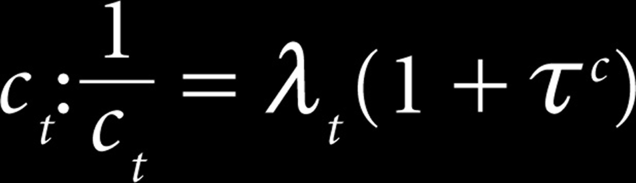
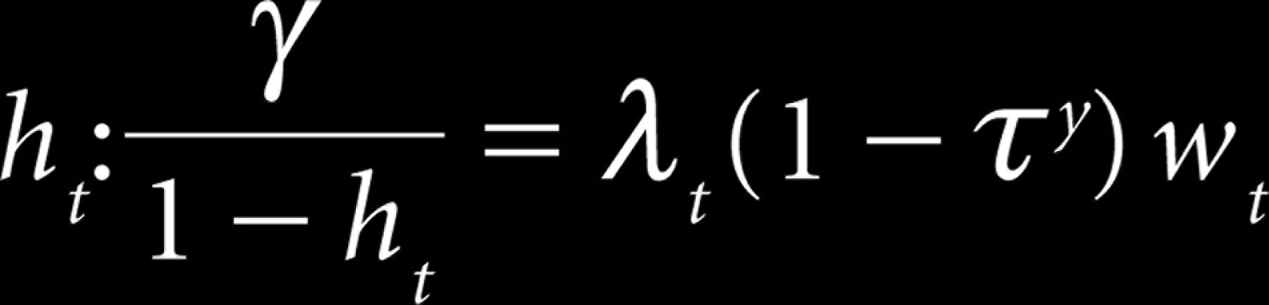


where λ t is the Lagrangean multiplier attached to household’s budget constraint in period t. The interpretation of the first-order conditions aforementioned is as follows: the first one states that for each household, the marginal utility of consumption equals the marginal utility of wealth, corrected for the consumption tax rate. The second equation states that when choosing labour supply optimally, at the margin, each hour spent by the household working for the firm should balance the benefit from doing so in terms of additional income generates, and the cost measured in terms of lower utility of leisure. The third equation is the so-called ‘Euler condition,’ which describes how the household chooses to allocate physical capital over time. The last condition is called the ‘transversality condition’ (TVC): it states that at the end of the horizon, the value of physical capital should be zero.
There is a representative firm in the economy, which produces a homogeneous product. The price of output is normalized to unity. The production technology is Cobb–Douglas and uses both physical capital, kt, and labour hours, ht, to maximize static profit

where At denotes the level of technology in period t. Note that we allow for the capital share to be time-varying.
Since the firm rents the capital from households, the problem of the firm is a sequence of static profit maximizing problems. In equilibrium, there are no profits, and each input is priced according to its marginal product, that is:
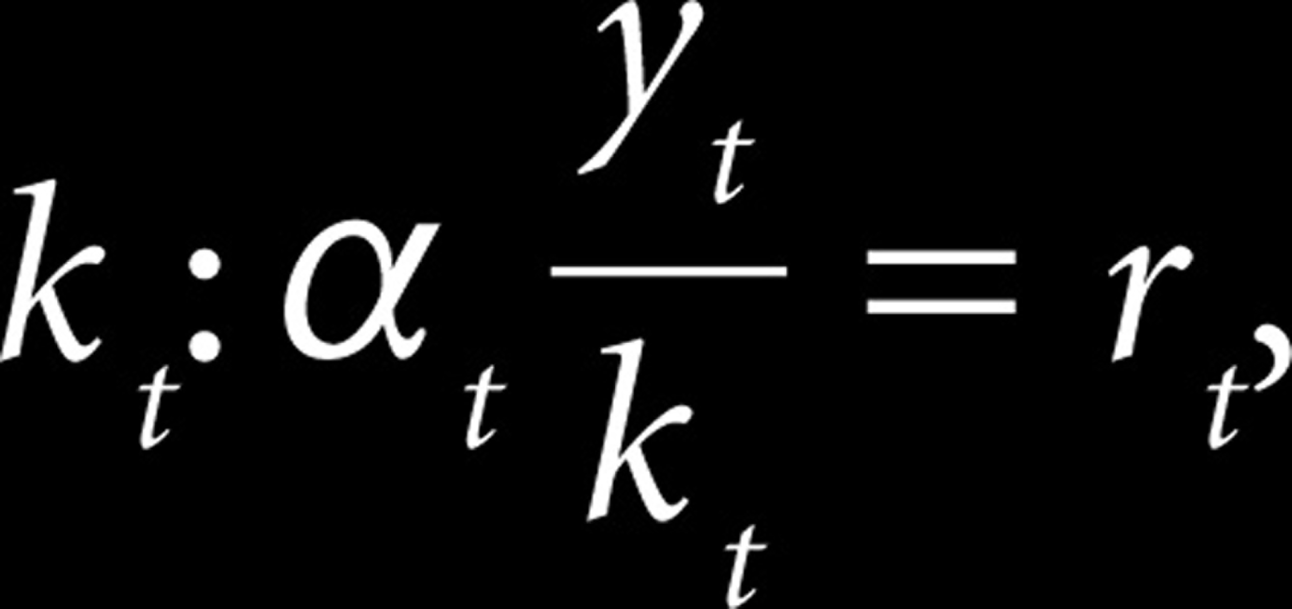
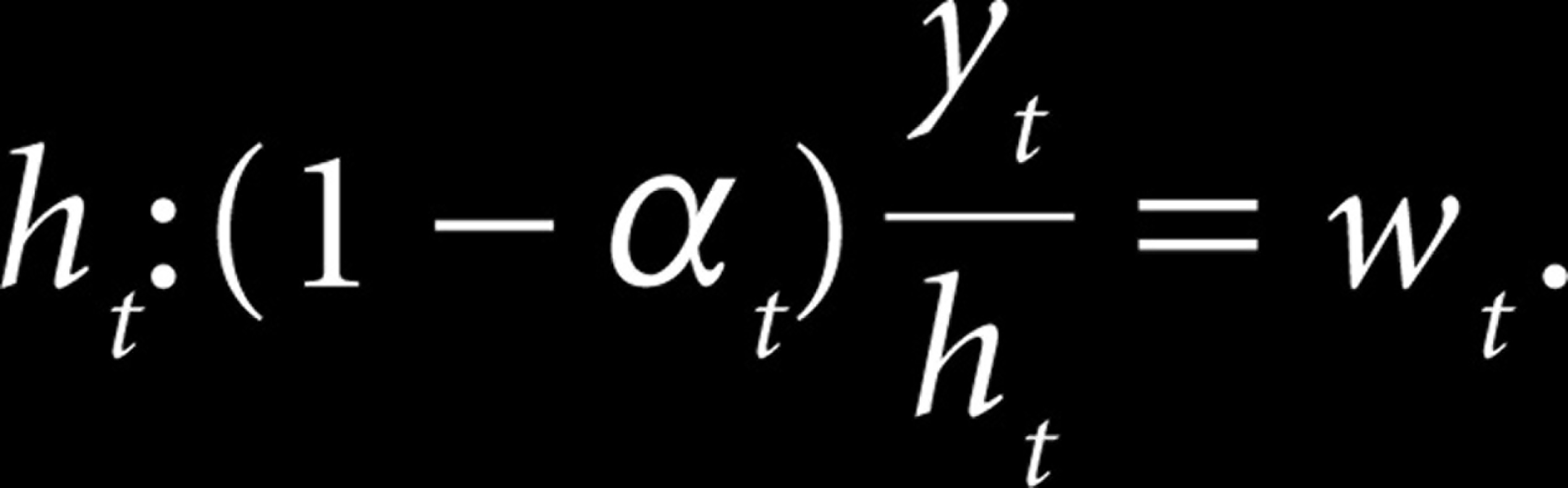
It is evident from the optimality conditions aforementioned that a positive shock to capital share directly (and indirectly—through output) increases the interest rate, and at the same time decreases the wage rate. This would have an immediate effect on the supply of the factors of production. Still, in equilibrium, given that the inputs of production are paid their marginal products, πt = 0, t.
In the model setup, the government is levying taxes on labour and capital income, as well as consumption, in order to finance spending on wasteful government purchases, and government transfers. The government budget constraint is as follows:

consumption tax, income tax rate and government consumption-to-output ratio would be chosen to match the average share in data. Finally, government transfers would be determined residually in each period so that the government budget is always balanced.
The exogenous processes for total factor productivity, At, and capital share, αt, will follow AR(1) processes in natural logarithms:


where A,θ are the steady-state values of the two processes, 0 < ρA, ρα < 1 are the respective persistence parameters, and the productivity innovations and changes to institutional quality are drawn from the following distributions:
For the given process followed by technology and capital share
Data and Model Calibration
To characterize business cycle fluctuations in Bulgaria, we will focus on the period following the introduction of the currency board (1999–2018). Quarterly data on output, consumption and investment were collected from National Statistical Institute (2019), while the real interest rate is taken from Bulgarian National Bank Statistical Database (2019). The calibration strategy described in this section follows a long-established tradition in modern macroeconomics: first, as in Vasilev (2016), the discount factor, β = 0.982, is set to match the steady-state capital-to-output ratio in Bulgaria, k / y = 13.964, in the steady-state Euler equation. The labour share parameter in steady-state, 1–α = 0.571, is obtained as in Vasilev (2017d), and equals the average value of labour income in aggregate output over the period 1999–2018. This value is slightly higher as compared to other studies on developed economies, due to the over-accumulation of physical capital, which was part of the ideology of the totalitarian regime, which was in place until 1989. Next, the average income tax rate was set to τy = 0.1. This is the average effective tax rate on income between 1999 and 2007, when Bulgaria used progressive income taxation, and equal to the proportional income tax rate introduced as of 2008. Similarly, the average tax rate on consumption is set to its value over the period, τc = 0.2.
Next, the relative weight attached to the utility out of leisure in the household’s utility function, γ, is calibrated to match that in steady-state consumers would supply one-third of their time endowment to working. This is in line with the estimates for Bulgaria (Vasilev, 2017a) as well over the period studied. Next, the steady-state depreciation rate of physical capital in Bulgaria, δ = 0.013, was taken from Vasilev (2016). It was estimated as the average quarterly depreciation rate over the period 1999–2014. Finally, the TFP process, and the process followed by capital share are estimated from the corresponding detrended series by running an AR(1) regression and saving the residuals. Table 1 beneath summarizes the values of all model parameters used in the article.
Model Parameters
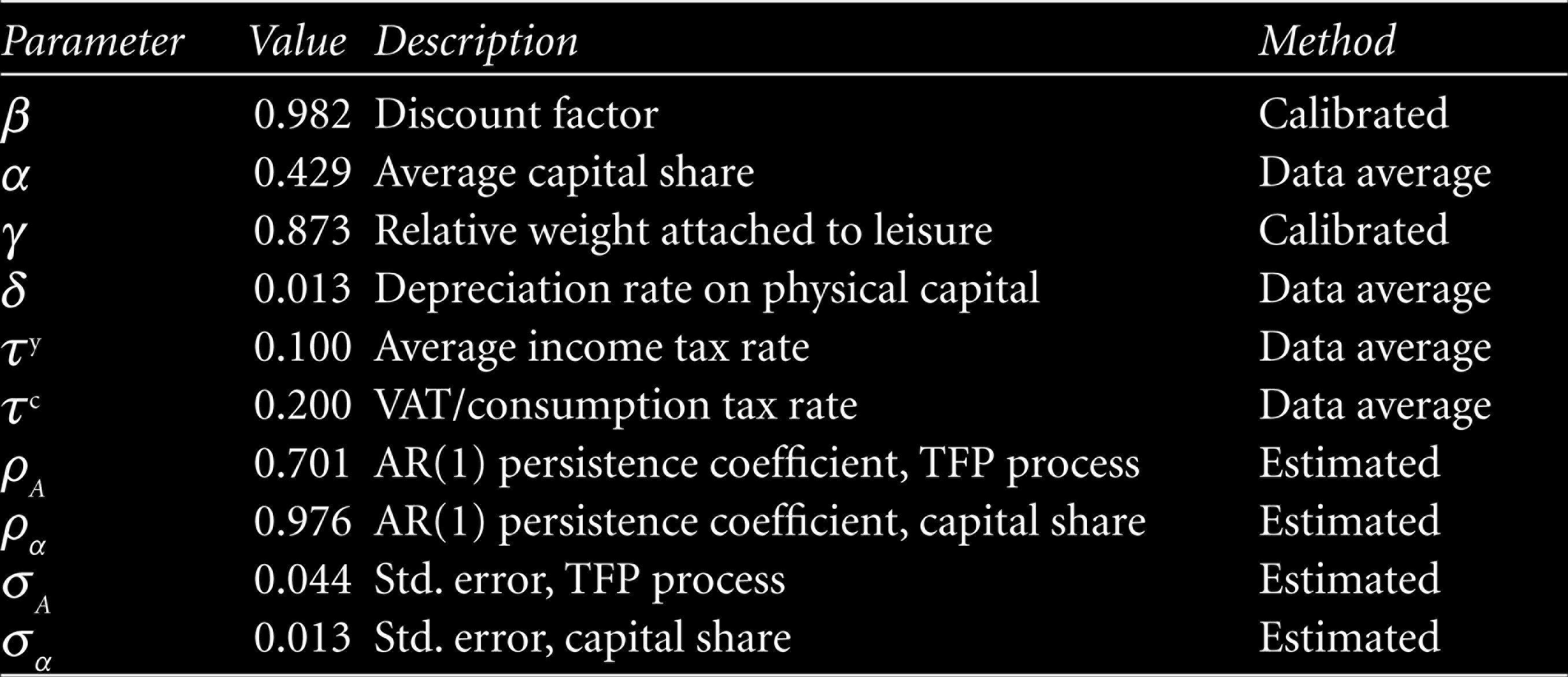
Model Parameters
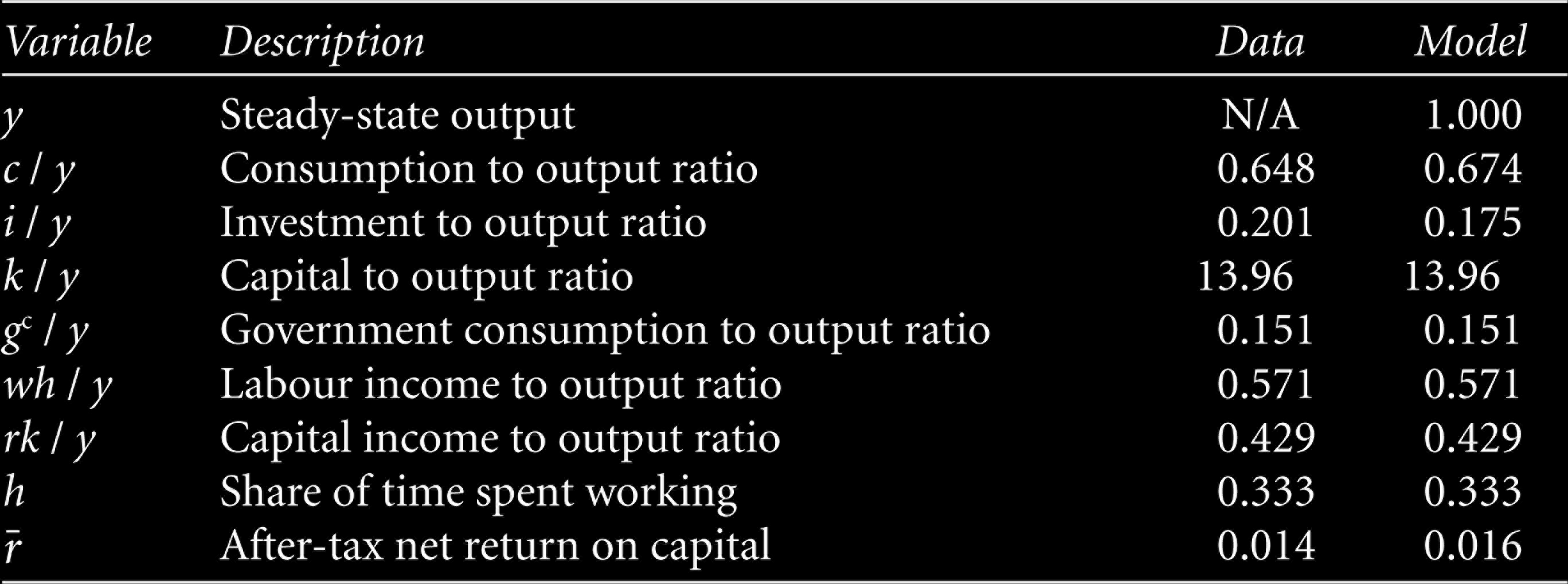
Once the values of model parameters were obtained, the steady-state equilibrium system solved, the ‘big ratios’ can be compared to their averages in Bulgarian data. The results are reported in Table 2 beneath. The steady-state level of output was normalized to unity (hence the level of technology A differs from one, which is usually the normalization done in other studies), which greatly simplified the computations. Next, the model matches consumption-to-output and government purchases ratios by construction. The investment ratios are also closely approximated, despite the closed-economy assumption and the absence of foreign trade sector. The shares of income are also identical to those in data, which is an artefact of the assumptions imposed on functional form of the aggregate production function. The after-tax return, where
Data Averages and Long-run Solution
Data Averages and Long-run Solution
Since the model does not have an analytical solution for the equilibrium behaviour of variables outside their steady-state values, we need to solve the model numerically. This is done by log-linearizing the original equilibrium (non-linear) system of equations around the steady-state. This transformation produces a first-order system of stochastic differential equations. First, we study the dynamic behaviour of model variables to an isolated shock to the total factor productivity process, and then we fully simulate the model to compare how the second moments of the model perform when compared against their empirical counterparts.
Impulse Response Analysis
This subsection documents the impulse responses of model variables to a 1% surprise innovation to the capital share. The impulse response functions (IRFs) are presented in Figure 1 on the next page. As a result of the one-time unexpected positive shock to the capital share, output increases upon impact directly. At the same time, interest rate increases, while wages decrease upon impact. The shock to the capital share is thus not just like a capital-biased technological progress, because at the same time it is biased against labour; A positive shock to the capital share is thus equivalent to a negative shock to the labour share. In other words, the increase in capital share increases the marginal return to capital and decreases the marginal return to labour. Those results follow from the Cobb–Douglas specification adopted for the production function.
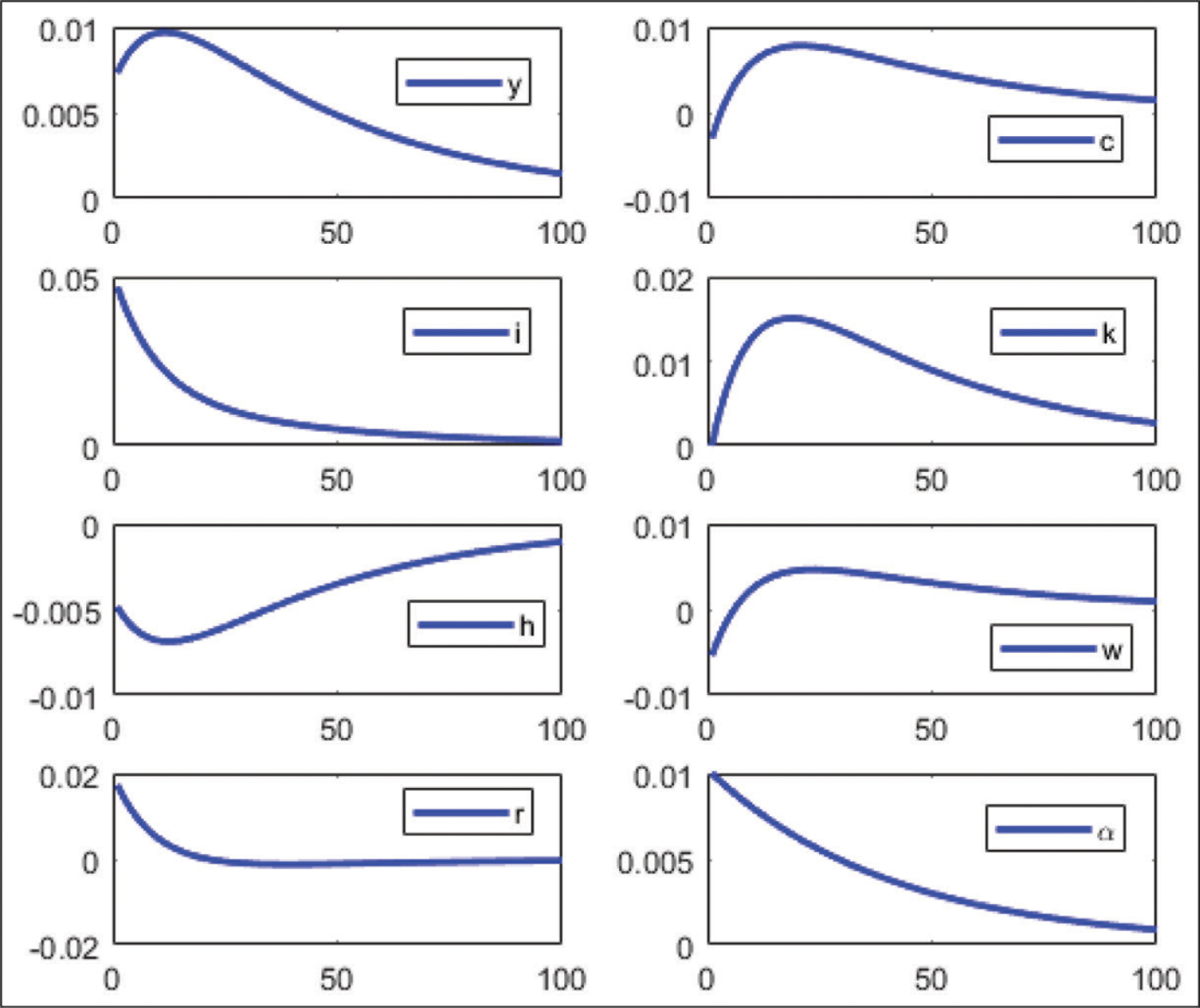
The increase in the after-tax return to capital motivates the household to increase investment and accumulating capital. In turn, the increase in capital input feeds back in output through the production function and that further adds to the positive effect of the capital share shock. On the other hand, the negative effect on the after-tax return to labour discourages the household from working, so hours fall. This effect feeds back into output through the production function and negatively reflects output. However, since a positive shock to capital share decreases the labour share in the production of output, the overall effect on output is still positive. Still, the counter-cyclical behaviour of labour supply creates a puzzle, as in data hours co-move with output. 6
Note that the increase in saving after the shock requires the household to temporarily decrease consumption. Thus, consumption drops upon impact of the shock, but then recovers as future output is still above its steady-state. As in the standard model, the transition dynamics of consumption follows the path of physical capital.
Over time, as capital is being accumulated, its after-tax marginal product starts to decrease, which lowers the households’ incentives to save. As a result, physical capital stock eventually returns to its steady-state, and exhibits a hump-shaped dynamics over its transition path. The rest of the model variables return to their old steady-states in a monotone fashion as the effect of the one-time surprise innovation in the capital share dies out.
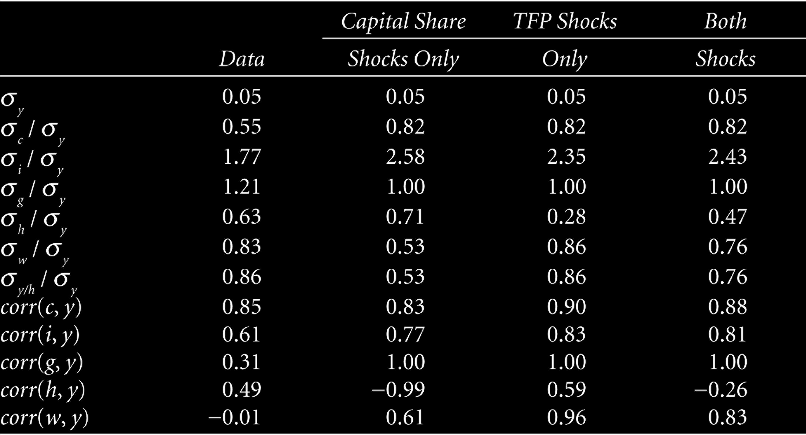
As in Vasilev (2017b, 2017e), we will now simulate the model 10,000 times for the length of the data horizon. Both empirical and model simulated data are detrended using the Hodrick and Prescott (1980) filter. Table 3 on the next page summarizes the second moments of data (relative volatilities to output, and contemporaneous correlations with output) versus the same moments computed from the model-simulated data at quarterly frequency. They simulate three specification: the first is with shocks to the capital share and no technology shocks, the second is the standard model with a fixed capital share parameter and technology shocks and the third specification is a set-up with both technology innovations and variations in the capital share.
Business Cycle Moments
Business Cycle Moments
In addition, to minimize the sample error, the simulated moments are averaged out over the computer-generated draws. As in Vasilev (2016, 2017b, 2017c), all models match quite well the absolute volatility of output. By construction, government consumption in the model varies as much as output. In addition, all three models generate consumption and investment volatilies that are too high as compared to data. In particular, with shocks to the capital share, investment volatility is larger. Still, the model is qualitatively consistent with the stylized fact that consumption generally varies less than output, while investment is more volatile than output.
With respect to the labour market variables, the variability of employment predicted by the model with varying capital share is a bit higher than that in data, but much larger than the volatility generated in a model with a fixed capital share. In addition, the increase in variability comes at the expense of the co-movement, as employment becomes counter-cyclical in the setup with shocks to the capital share parameter. In terms of wage volatility, the model with stochastic capital share generates too little variability, and is dominated by the model driven by technology shocks. These results are yet another confirmation that the perfectly competitive assumption (e.g., Vasilev, 2009) as well as the benchmark calibration here does not describe very well the dynamics of labour market variables, even when we allow for stochasticity in the capital share parameter.
Next, in terms of contemporaneous correlations, all models systematically over-predicts the pro-cyclicality of the main aggregate variables—consumption, investment and government consumption. This, however, is a common limitation of this class of models. The model with shocks to the capital income share even gets the cyclicality of hours completely wrong. With respect to wages, all models predict moderate to strong pro-cyclicality, while wages in data are acyclical. Again, this shortcoming is well known in the literature and an artefact of the wage being equal to the labour productivity in the model.
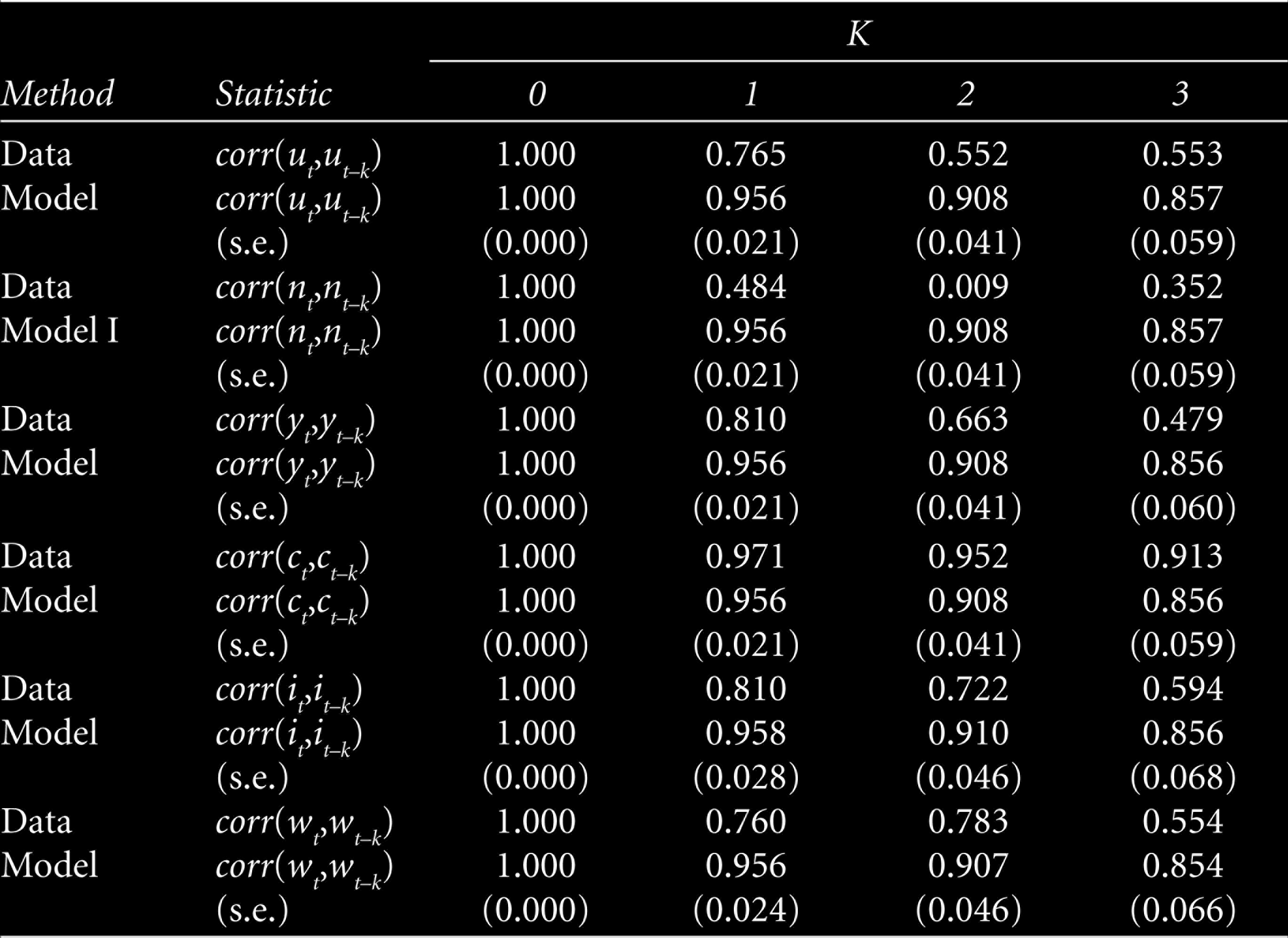
In the next subsection, as in Vasilev (2015), we investigate the dynamic correlation between labour market variables at different leads and lags, thus evaluating how well the model matches the phase dynamics among variables. In addition, the autocorrelation functions (ACFs) of empirical data, obtained from an unrestricted VAR(1), are put under scrutiny and compared and contrasted to the simulated counterparts generated from the model.
This subsection discusses the auto-(ACFs) and cross-correlation functions (CCFs) of the major model variables. The coefficients empirical ACFs and CCFs at different leads and lags are presented in Table 4 beneath against the averaged simulated AFCs and CCFs. 7 To economize on space, we only present the model with stochastic capital income, and no technology shocks.
Autocorrelations for Bulgarian Data and the Model Economy
Autocorrelations for Bulgarian Data and the Model Economy
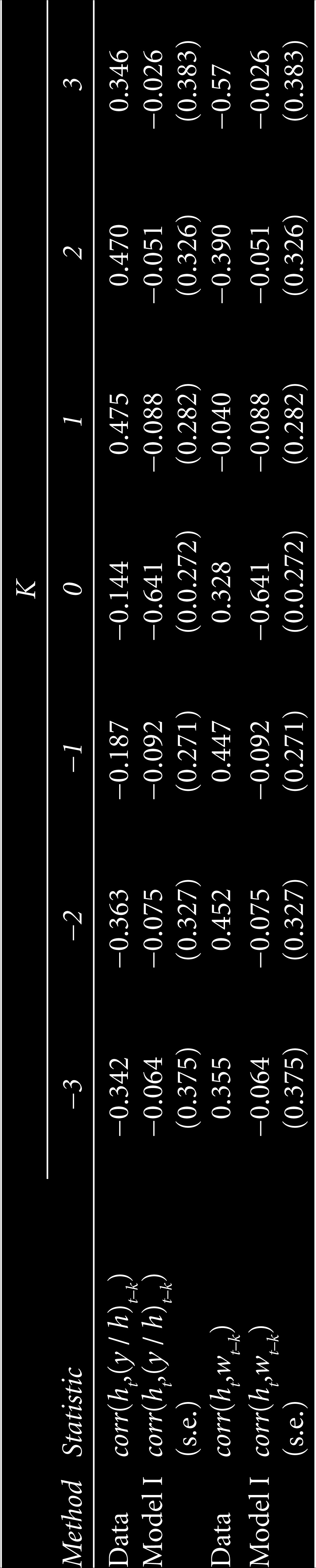
As seen from Table 4 earlier, the model compares relatively well vis-a-vis data. Empirical ACFs for output and investment are slightly outside the confidence band predicted by the model, while the ACFs for total factor productivity and household consumption are well-approximated by the model. The persistence of labour market variables are also relatively well-described by the model dynamics. Overall, the model with a stochastic capital share generates too much persistence in output and both employment and unemployment, and is subject to the criticism in Nelson and Plosser (1982), Cogley and Nason (1995) and Rotemberg and Woodford (1996b), who argue that the RBC class of models do not have a strong internal propagation mechanism besides the strong persistence in the TFP process. In those models, for example, Vasilev (2009), and in the current one, labour market is modelled in the Walrasian market-clearing spirit, and output and unemployment persistence are low. Next, as seen from Table 5 beneath, over the business cycle, in data labour productivity leads employment. The model with stochastic capital income share, however, cannot account for this fact. 8 As in the standard RBC model, the shock to the capital share parameter in this article can be also regarded as a factor shifting the labour demand curve, while holding the labour supply curve constant. Therefore, the effect between employment and labour productivity is only a contemporaneous one.
Dynamic Correlations for Bulgarian Data and the Model Economy
We allow for a time-varying capital share into a real-business-cycle setup with a government sector. We calibrate the model to Bulgarian data for the period following the introduction of the currency board arrangement (1999–2018). We investigate the quantitative importance of the variability in capital share for cyclical fluctuations in Bulgaria. In particular, allowing for a stochastic capital share in the model increases variability of investment and employment, at the cost of decreasing the volatility of wages, and causing employment to become countercyclical.
Footnotes
Declaration of Conflicting Interests
The author declared no potential conflicts of interest with respect to the research, authorship, and/or publication of this article.
Funding
The author received no financial support for the research, authorship, and/or publication of this article.