
Abstract
Objective
To investigate the capability of various study designs to determine the sensitivity of a disease screening test.
Methods
Quantities that can be calculated from these designs were derived and examined for their relationship to true sensitivity (the ability to detect unrecognized disease that would surface clinically in the absence of screening) and overdiagnosis.
Results
To examine the sensitivity of one test, the single cohort design, in which all participants receive the test, is particularly weak, providing only an upper bound on the true sensitivity, and yields no information about overdiagnosis. A randomized design, with one control arm and participants tested in the other, that includes sufficient post-screening follow-up, allows calculation of bounds on, and an approximation to, true sensitivity and also determination of overdiagnosis. Without follow-up, bounds on the true sensitivity can be calculated. To compare two tests, the single cohort paired design in which all participants receive both tests is precarious. The three arm randomized design with post screening follow-up is preferred, yielding an approximation to the true sensitivity, bounds on the true sensitivity, and the extent of overdiagnosis of each test. Without post screening follow-up, bounds on the true sensitivities can be calculated. When an unscreened control arm is not possible, the two-arm randomized design is recommended. Individual test sensitivities cannot be determined, but with sufficient post-screening follow-up, an order relationship can be established, as can the difference in overdiagnosis between the two tests.
Introduction
Sensitivity, the proportion of screened subjects with the target condition with a positive screening result, is one of the key operating characteristics of screening tests. Although high sensitivity is not sufficient or necessary for a screening test to improve disease outcome, it is important to determine sensitivity accurately before the test is used, because of the high costs associated with an inaccurate test.
A number of study designs can be contemplated to determine the sensitivity of a single test, or to compare the sensitivities of two or more tests 1 , but many have limitations.2–4 This paper aims to investigate several study designs for determining test sensitivity in a screening programme. It is envisioned that a study involves multiple screening rounds, and the entire screening episode from test result to diagnostic confirmation is considered. The term sensitivity as used in this paper is therefore the episode sensitivity in a screening programme with several rounds.
It is assumed that a test detects cases early, does not prevent clinical disease by detecting true precursor lesions, that compliance with screening is perfect, and that preliminary estimates of test operating characteristics are available.5–9 The focus is on determining true test sensitivity (the ability to detect disease before it progresses to recognizable, symptomatic stages), or comparing the sensitivities of two tests, in those screened. Another important goal is to determine the amount of overdiagnosis (detection of disease that would not surface clinically in the absence of screening) from a test, or the difference in overdiagnosis between two tests. Our focus is the application of screening for cancer, though most of the principles we discuss apply to screening for other diseases.
Methods
Standard mathematical manipulations are used to investigate the limitations of various study designs for determining sensitivity. Designs of decreasing rigour, from multi-arm randomized trials to single cohort studies, are sequentially considered. Quantities that can be calculated from each design are scrutinized for their relationship to true sensitivity. The capability of the designs to determine overdiagnosis is also examined. For purposes of illustration, random variation is ignored.
Results
Determining the sensitivity of a single test
Single Test Disease Case Subset Definitions.
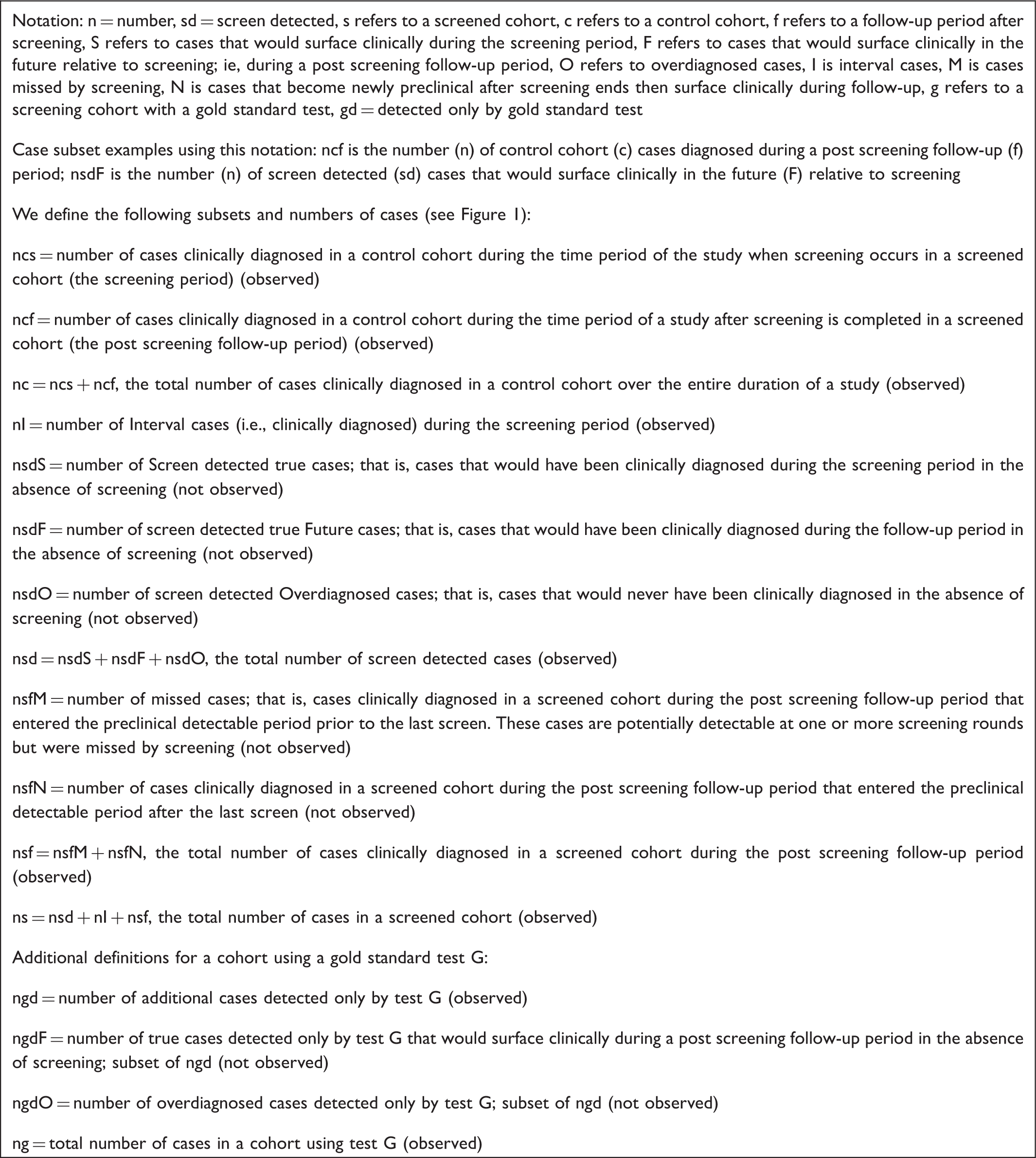
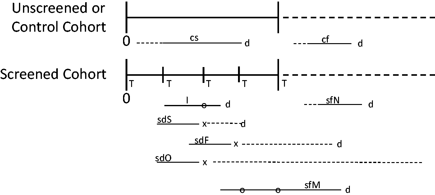
Subgroups of cases in screened and unscreened cohorts relevant to determining the sensitivity of a single test. Five rounds of screening are depicted, designated by T. x = time of screen detection; d = time of clinical diagnosis; o = false negative screen. Horizontal lines represent the duration of the pre-clinical detectable phase (PDP) of the disease. For the cf cases, the PDP could have started before screening began, during the screening period, or after screening ended. The sfN cases enter the PDP after screening ended. For all other case subgroups, the PDP could have started before screening began or during the screening period. For screen detected cases sdS and sdF, the dotted horizontal portion of the PDP after the x is the lead time. See Box 1 for subgroup definitions.
A true clinical case is defined as one that would be clinically diagnosed due to signs or symptoms during the time frame of a particular study, if there were no screening. The true sensitivity of a test (ST) is then the number of screen-detected true clinical cases in the preclinical detectable phase (PDP) during the screening period or screening phase of a study, divided by the number of all true clinical cases in the PDP during the screening period.
10
The numerator is the sum of the number of screen detected cases that would have surfaced clinically during the screening period (nsdS), and those that would have surfaced during post screening follow-up (nsdF), if there were no screening. The denominator includes these cases, plus the interval cases (nI), plus the cases that were in the PDP at the time of one or more of the screens but were missed by screening, and are clinically diagnosed during post screening follow-up (nsfM). Therefore,

ST cannot be calculated directly because nsdS, nsdF, and nsfM are not observed. The sdS and sdF cases cannot be individually identified as they are subsets of all the screen detected cases (nsd), that also includes any overdiagnosed cases (nsdO). Similarly, the sfM cases are a subset of the totality of clinical cases that are diagnosed after screening ends. These are also not identifiable because this totality of cases comprises cases missed by the screen (sfM cases) plus cases that entered the PDP after the last screen but then surfaced clinically (sfN cases).
We aimed to determine study designs that can provide the necessary information to calculate ST and to identify shortcomings in study designs that preclude such calculation.
Ideal three arm randomized design
A three arm randomized design that, in principle, yields the necessary information, is depicted in Figure 2. Participants in the control arm are not screened. Those in the T arm are screened using test T for some time period. The third arm (G) duplicates the T arm, but additionally a gold standard test G with 100% true sensitivity relative to test T is performed on all participants at the last screening round. In an ideal setting, all participants are followed to death to identify all clinically diagnosed cases. We assume all arms are of equal size.
Three arm randomized design to determine the sensitivity of a screening test. R = randomization; T = screening test T performed; G = gold standard screening test G performed.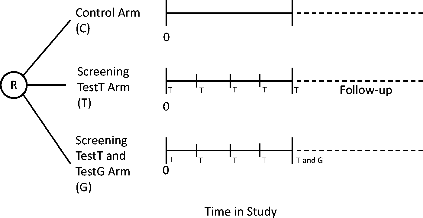
In the numerator of expression [1], nsdS and nsdF are not individually observable, but it is possible to observe the total number of screen detected cases nsd. The number of overdiagnosed cases can be determined as the difference between the total numbers of cases in arms T and C, ie:

From the definition of nsd and expression [2], the numerator of ST is then nsdS + nsdF = nsd − nsdO = nc − nI − nsf. Again using expression [2] and the definition of nsf in Box 1, the denominator of ST is nsdS + nsdF + nI + nsfM = nc − nI − (nsfM + nsfN) + nI + nsfM = nc − nsfN. Thus:

Only nsfN in expression [3] is not directly observed. The additional information required to determine nsfN can be obtained from arm G in this design (Appendix 1, available online). The resulting expression for the true sensitivity in terms of observable quantities is:

Two arm randomized design
The three arm design will rarely, if ever, be feasible, due to the non-existence of a 100% sensitive test G, the impracticality of performing two tests in one of the study arms, or the cost of a third arm. An alternative is the two arm randomized design, involving only arms T and C, in Figure 2. Both arms are assumed to be of equal size and all participants are followed to death.
Because the information from arm G is not available in this design, nsfM cannot be determined and ST cannot be calculated. However, after several screens, most of the detectable cases will have been identified, so nsfM would be small. An approximation is nsfMA = the number of clinical cases diagnosed in the screened arm in the first two years after screening ends. Two years is arbitrary, and a sensitivity analysis could be performed.
In practice all study participants are never followed to death. However, if follow-up is sufficiently long after screening stops, and the cumulative number of cases in each study arm becomes the same, nsdO = 0. 11 Alternatively, if the difference in total cases between the two arms becomes constant, nsdO follows from expression [2].12–14
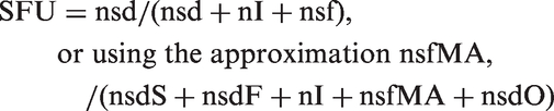
A practical design then is a two arm randomized trial with sufficiently long follow-up to determine nsdO. From expression [1], an approximation to the true sensitivity is

Although only an approximate true sensitivity is obtained, it is possible to determine bounds on ST (Appendix 2, available online). An upper bound is STU = (nsd − nsdO)/(nsd − nsdO + nI) and a lower bound is STL = (nsd − nsdO)/(nsd − nsdO + nI + nsf).
If there is no post screening follow-up, nsdO and nsfM cannot be determined, nor ST, STU, or STL. ST, STU and STL all reduce to SR = 1 − (nI/ncs). An upper bound can be calculated SU = nsd/(nsd + nI) > STU. If there is no follow-up, but the number of cases in each inter-screening interval stabilizes to some value, substituting this value for nsf in the expression for STL yields an approximate lower bound.
Single cohort design
Available information is limited to that from the T Arm in Figure 2, so the missed cases and the overdiagnosed cases cannot be determined. Referring to expression [1], the only term that can be obtained is nI. Therefore ST cannot be calculated in this design. If there is follow-up, a candidate sensitivity value is:
If there is no follow-up, SU can be calculated as above. Comparing with expression [1], it is clear that neither quantity is equal to ST. This design provides little useful information.
Comparing the sensitivities of two tests
Ideal five arm randomized design
When two tests are to be compared, and there is no screening test of proven benefit, an unscreened control group is desirable. Based on the above single test discussion, the full information needed to determine the true sensitivities of each test can be obtained by randomizing participants into one of five arms (Figure 3). One arm serves as a control, participants in the T1 arm are screened with test1, participants in the G1 arm are screened with test1 and also at the last round with a gold standard test G1, participants in the T2 arm are screened with test2, and participants in the G2 arm are screened with test2 and also at the last round with a gold standard test G2. All are followed to death. We assume equal numbers of participants and equal periods of screening in each arm.
Five arm randomized design to determine the sensitivities of two screening tests. R = randomization; T1 = screening test1 performed; T2 = screening test2 performed; G1 = gold standard screening test G1 performed; G2 = gold standard screening test G2 performed.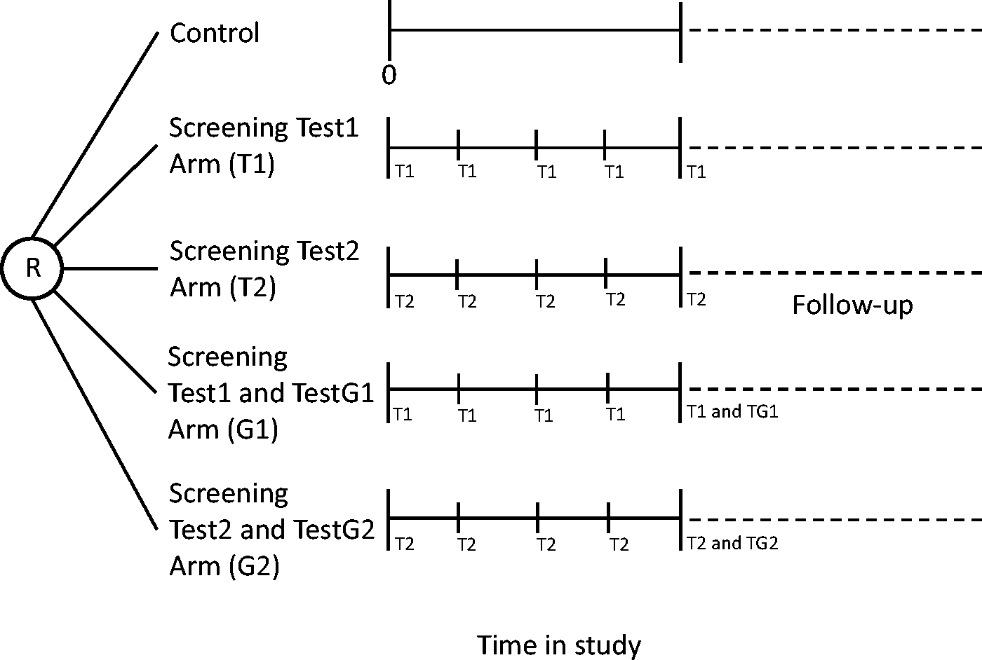
The types of cases are defined as for the single test situation. From the control arm there is ncs and ncf, and their sum nc. Let i = 1,2 index the two tests and all the component terms in expressions [1–4] be defined as for the single test designs, except relative to test Ti. Each test arm is compared with the control arm, to determine nsdOi = nsi − nc. From expression [1], the true sensitivity of Ti is:

This can be expressed using information from arm Ti, arm Gi, and the control arm in terms of observable quantities as STi = (nc − nsfi − nIi)/(nc − nsfi + nsi + ngdi − ngi).
This design thus allows the determination of the true sensitivity of each test, direct comparison of the true sensitivities, and observation of the number of cases overdiagnosed by each test.
Four arm randomized design
If one of the tests has been shown to improve health outcomes, an unscreened control arm is not ethical. A possible design involves the four screening arms in Figure 3 and post-screening follow-up of sufficient duration to establish equivalence or a constant difference in total cases among the arms. Without control arm information, it is not possible to determine the individual test sensitivities (STi), nor the numbers of overdiagnosed cases (nsdOi).
Let the difference in interval cases between the two tests be ΔnI = nI2 − nI1, the difference in overdiagnosed cases be ΔnsdO = ns2 − ns1, and the difference in missed cases be ΔnsfM = nsfM2 − nsfM1. All three quantities can be calculated in this design, potentially enabelling the two tests to be ranked (Appendix 3, available online). Specifically, if all three differences have the same sign, one of the tests has more interval cases, more missed cases, and more overdiagnosed cases than the other. The other test would be preferred.
It is also possible to rank the sensitivities of the two tests in this design. It can be shown (Appendix 3, available online) that:
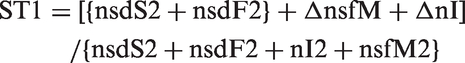
The part of expression [7] in curly brackets is the definition of ST2 from expression [6]. Therefore if ΔnsfM + ΔnI is positive, ST1 > ST2 and vice versa.
Three arm randomized design
The five and four arm designs described above would rarely be feasible for reasons noted in the discussion of the three arm trial for a single test. We are not aware of any that have been conducted; they were presented for illustrative reasons. If a control arm is feasible, a three arm randomized design for comparing two tests is the next best choice. 15 This design comprises arms T1, T2, and Control in Figure 3. Again, it is assumed that the numbers of participants in each arm are equal, and that follow-up is sufficiently long to establish either equivalence or a constant difference in total cases between each screened arm and the control arm.
The individual numbers of overdiagnosed cases can be calculated from observed quantities as nsdOi = nsi − nc. However, without gold standard test information, the missed cases nsfMi are not known, so the true sensitivities STi cannot be found, but an approximation, bounds, and ranking are possible. By analogy with the one test setting, the approximate quantities nsfMAi can be determined to yield approximate sensitivities STAi = (nsdi − nsdOi)/(nsdi − nsdOi + nIi + nsfMAi), and upper and lower bounds STUi and STLi can be obtained for each test as in Appendix 2, available online. If the intervals (STL1, STU1) and (STL2, STU2) are very narrow and substantially overlap, it can be concluded that ST1 and ST2 are equal for all practical purposes. Alternatively, if STU2 < STL1 then STL2 < = ST2 < = STU2 < STL1 < = ST1 < = STU1 and it follows that ST2 < ST1 (or vice versa).
If there is no post-screening follow-up, STi, STAi, and nsdOi cannot be determined, again analogous to the two-arm design in the one test setting, but upper and lower bounds can be calculated.
Two arm randomized design
If an unscreened control arm is not ethical, the two-arm randomized design with follow-up still has utility for guiding screening policy. 16 The types of cases considered are the same as for the T1 and T2 arms of the four-arm design. The screen detected (nsdi), interval (nIi) and follow-up (nsfi) cases for both tests are observed, but it is not possible to determine the overdiagnosed cases or missed cases, because there are no control arms or gold standard test arms. Therefore, true and approximate sensitivities cannot be determined.
The difference in overdiagnosed cases can be calculated as ΔnsdO = ns2 − ns1, and an ordering of the sensitivities is possible. An argument similar to that for the four-arm design (Appendix 3, available online) applies here as well, and the relationship in expression [7] holds. Although nsfMi cannot be determined, in the numerator of expression [7] the sum ΔnsfM + ΔnI can be obtained as the observable quantity (ns2 − ns1) − (nsd2 − nsd1) using the definition of nsi and the fact that nsfN1 = nsfN2. If this quantity is non-negative, ST1 ≥ ST2. Otherwise, ST2 > ST1.
If there is no post-screening follow-up, the only available data are nsdi and nIi. The difference in interval cases is observed, but without knowing the difference in overdiagnosed cases, this is of questionable value. The upper bounds SUi = nsdi/(nsdi + nIi) can be calculated, but no lower bound other than zero is apparent, so the order relationship between the STi cannot be determined.
Single cohort paired design
Using the concepts developed above, it is possible to identify shortcomings in the most frequently used design.17–22 All participants are in one cohort and each receives both screening tests. Overdiagnosed cases cannot be determined because there is no control arm, and post-screening follow-up provides no useful information because the subsequent occurrence of disease cannot be related to the effect of screening by either test individually. The cases missed individually by each test also cannot be determined, even if there were follow-up, because the cases that surface clinically after screening ends are a mixture of those missed by both tests plus newly developing cases, and the components cannot be separated in this design.
The individual interval cases for each test and the difference in interval cases between the tests are not observable because the observed interval cases are either missed by both tests, or are newly preclinical during the interval. As two tests are used on the same people, some cases detected by only one of the tests would not be detectable if only the other test were used, while some cases that would be detected by one test are found earlier by the other test and so are censored relative to the first test. There are 17 types of cases to be considered (Appendix 4, available online).
We consider the relationship between a candidate sensitivity quantity for test1 that can be calculated from this design versus ST1. Results for test2 follow similarly. The true sensitivity of test1 cannot be determined, but a frequently reported result from such studies is all cases detected by test1 divided by all cases identified during the study, designated SP1. 1 However, ST1 and SP1 are not equivalent, and the order relationship between them is not obvious (Appendix 4, available online).
Thus although this study design is the least expensive comparison of two or more screening tests, it cannot yield reliable true sensitivities of either test individually, nor any order relationship between the sensitivities. This design also provides no information on the magnitude of overdiagnosis of either test.
Discussion
Determining the true sensitivity of a screening test and comparing the sensitivities of two screening tests are difficult. For evaluating a single test, the single cohort design provides data for only an upper bound on the true sensitivity, and yields no information about overdiagnosis. A randomized design with sufficiently long post screening follow-up allows calculation of an approximate true sensitivity, bounds on the true sensitivity, and determination of the level of overdiagnosis. Without post screening follow-up, it is still possible to calculate weaker bounds on the true sensitivity.
For comparing the sensitivities of two screening tests, the single cohort paired design is problematic, as individual test sensitivities and overdiagnosed cases cannot be determined. Formulating screening policy based on this study design is precarious. The three arm randomized design is superior when there is no standard, but two proposed tests. Using this design with post screening follow-up, the extent of overdiagnosis of each test can be determined. Approximate true sensitivities of each test can be obtained and compared directly, as can bounds on the true sensitivities. Without post screening follow-up, only weaker bounds on the true sensitivities are available, and there is no information on overdiagnosis. When circumstances do not permit an unscreened control arm, a practical design is the two arm randomized design. Individual test sensitivities cannot be determined, but an order relationship can be established, as can the difference in overdiagnosed cases between the two tests, provided post screening follow-up data are collected.
One limitation of our approach is the assumption of 100% attendance at screening. In a real life screening setting this is unlikely to occur, and the resulting nonresponse is well known to cause selection bias between attenders and non-attenders, often in the form of healthy screenee bias. This can pose both practical and theoretical problems, especially when a study extends over several rounds of screening. In the two arm design for comparing two tests, for example, if the disease target was colorectal cancer and one arm used an invasive test such as colonoscopy while the other used a blood based test, the different characteristics of the two tests could influence the willingness of potential participants to enter the study, or cause differential drop out as the study progressed. While imperfect compliance is a very real practical issue, it is likely to occur with whatever study design is used. Low compliance could affect the absolute value of the sensitivity, but it is not clear that this bias affects the relative strengths of the various designs we have discussed. We have assumed ideal compliance only for the purpose of simplifying the illustration of the relationships among the designs.
We have not addressed the issue that the relationships among the various components of sensitivity are likely to depend on the design parameters of the screening study, such as the number of screening rounds and the interval between screens. The magnitude of non-diagnosed preclinical cases, in particular the missed (M) cases in this formulation, decreases compared with the accumulated number of screen detected cases with longer study duration. Hence, the contribution of these cases becomes proportionately less important, and overdiagnosis becomes an increasing problem as the number of screening rounds increases. Assessment of these relationships is an important subject for future investigation.
A prevalent assumption is that a test with greater sensitivity than another is necessarily better, but the test with lower sensitivity might be as good, if it can detect the subset of cases whose outcome is improved by early therapy. Determining the sensitivity of a screening test for true, not overdiagnosed, disease is only one consideration when assessing a new screening test. Other process measures should also be determined, in particular, the specificity of the test, in order fully to evaluate test performance. Ultimately, the most important consideration is whether use of the test results in improved disease outcome, even though this may require considerable time and a large study to determine unequivocally. Although demonstration that a new test has greater sensitivity than an old test is often touted as an important approach to decision-making, our findings indicate the danger of relying exclusively on this approach.
Conclusion
For determining the sensitivity of a single test, the single cohort design provides data for only an upper bound on the true sensitivity, and yields no information about overdiagnosis. A randomized design with sufficient post screening follow-up is superior. To compare the sensitivities of two tests, the single cohort paired design is problematic, as individual test sensitivities and overdiagnosed cases cannot be determined. Formulating screening policy based on this study design is precarious. The three arm randomized design is better when there is no standard, but two proposed tests. If an unscreened control arm is not feasible, the two arm randomized design is a practical choice.
Footnotes
Acknowledgements
This research received no specific grant from any funding agency in the public, commercial, or not-for-profit sectors.
Conflicts of interest
None
References
Supplementary Material
Please find the following supplemental material available below.
For Open Access articles published under a Creative Commons License, all supplemental material carries the same license as the article it is associated with.
For non-Open Access articles published, all supplemental material carries a non-exclusive license, and permission requests for re-use of supplemental material or any part of supplemental material shall be sent directly to the copyright owner as specified in the copyright notice associated with the article.