
Abstract
The decision on whether to implement a 20-year screening programme for a cancer requires weighing the harms and costs against the health benefits (such as the number of cancer deaths averted every year). The evidence of the benefits is often based on a single-number summary, such as the mortality reduction over the entire follow-up time in a single trial, or an average of such one-number measures from a meta-analysis of several trials. There are several problems associated with using the traditional one-number summaries from trials to deduce the yearly mortality reductions expected from a sustained screening programme. We here propose using a rate ratio curve, and its complement (a mortality reduction curve), to address the mortality impact (timing, magnitude, and duration) of a screening programme. This curve is easy to interpret, as it shows when mortality reductions begin, how big they are, and how long they last. We illustrate when and how such rate ratio curves from screening trials could be computed, and how they could be used to compare reduction patterns expected with different screening regimens. We encourage trialists to report the necessary data to arrive at such projections.
Introduction
Making a decision on whether or not to implement a 20-year screening programme for a cancer requires weighing the harms and costs against the health benefits (such as the number of cancer deaths averted every year). The evidence of the benefits is often based on a single-number summary, such as the mortality reduction over the entire follow-up time in a single trial, or an average of such one-number measures from several trials. We recommend against using such one-number summaries to deduce the yearly mortality reductions expected from a sustained screening programme.
As detailed below, we base this recommendation on several reasons, all stemming from the characteristic time-pattern of the mortality reductions produced by any particular screening programme, and the affected time-window in question. First, the reductions do not begin in year one, and if/when they do reach a ‘constant’ level, they do not remain at this level indefinitely. Thus the full pattern (ie. the timing, magnitude and duration of the reductions) cannot be adequately quantified by one number. In addition, the pattern is specific to the screening regimen (eg. the number of screens and spacing between them) employed. For example, 20 annual screens might produce yearly reductions that start at year 5, and extend over possibly 25 years; 10 annual rounds would produce similar yearly reductions starting at about the same time, but extending over a shorter span, possibly 15 years. Compared with 10 annual screenings, the yearly reductions produced by 10 biennial screenings are expected to be smaller but over a longer period of time.
We here address the task of projecting the mortality impact of a screening programme. In Section 1, we propose using a rate ratio curve, instead of a single-number summary, to fully describe the expected timing, magnitude and duration of this impact. In Section 2, we identify trials that have had sufficient rounds of screening allowing us to estimate the asymptote of the curve for a programme with similar spacing of screens. We also give examples to illustrate how much underestimation is involved in the traditional measure. In Section 3, we show how it is possible to use an existing model (previously used for other purposes), and available trial data to project the programme impact, as well as compare reduction patterns produced by regimens with different spacings from those used in trials. Finally, we call on trialists to report necessary data to compute this rate ratio curve.
1 The mortality reduction curve, and its shape
The time lag and the affected age window
Consider a cohort of persons who, beginning at age 50, are invited to be screened
annually for a cancer until they reach age 69. The mortality impact of the programme is
the difference in the yearly number of cancer deaths in the absence of screening (when no
one is invited to be screened) versus in the presence of screening (when everyone is). We
graph this impact in the affected age window in Figure 1(a). Impact of a hypothetical 20-year
screening programme measured (a) in absolute numbers of cancer-specific deaths
averted and (b) as rate ratios and as percentage reductions.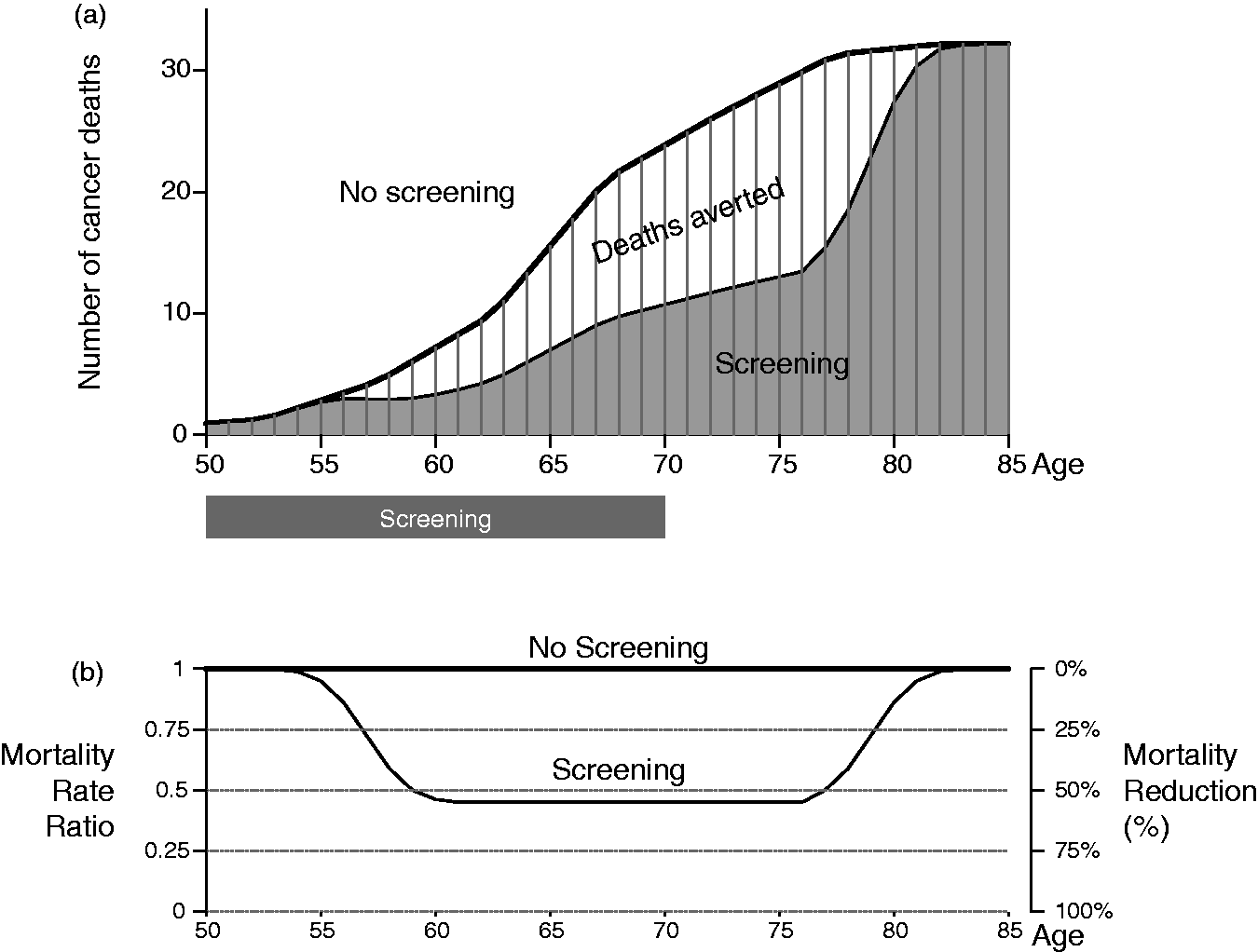
The first notable feature is the time lag between when a screening programme starts and when the mortality reduction first manifests. Unlike most medical interventions those produce a virtually immediate effect (within hours, days or weeks), cancer screening generates mortality reductions that only become evident several years after the onset of screening.1–5 The first screen (say at age 50) detects, and the resulting earlier therapy eradicates, some cancers that otherwise would have proved fatal several years later (from say 55 to 63). Presumably, the average delay would be longer for cancers of the breast and prostate, and shorter for more aggressive cancers, such as that of the lung. The width of the reduction ‘wave’ (8 years in our example) reflects the variation in cancer stages at detection and in the rates at which cancers would have progressed otherwise.
Mortality reductions produced by subsequent annual screens (at ages 51, 52, … , 69) occur even later (from say 56 to 64, 57 to 65, … , 74 to 82). After the effect of the last screen disappears, cancer mortality rates return gradually (from say 78 to 85) to those in the absence of screening. Thus, the 20 screens affect possibly 35 age-bins in the age-span 50 to 85.
The total number of deaths averted in that span is shown as the white area in Figure 1(a). The total number of years gained is the sum of the products of the age-specific number of deaths averted and the age-specific remaining life expectancies. For costing purposes, this total can be averaged over the number averted, invited, or screened.
The mortality rate ratio curve
Another way to display the same mortality reductions in Figure 1(a) is through a rate ratio curve, as in Figure 1(b). The yearly ratio is calculated as the yearly number (or rate) of cancer deaths in the presence of screening divided by the yearly number (or rate) of cancer deaths in the absence of screening. Each yearly ratio can be thought of as the fraction of fatal cancers that could not be helped by screening. Their complements, usually expressed as percentages, represent the yearly mortality reductions.
If the yearly number of fatal cancers remains constant throughout the screening programme, the rate ratio curve should exhibit a bathtub shape: it would be close to constant for a large portion of the age-window where the effect of sustained screening is manifest. Little mortality impact is expected in the early portion, ie. before the deaths averted by the first screen would have otherwise occurred, and again in the late portion, ie. long after the deaths averted by the last screen would have otherwise occurred. By describing the timing, magnitude and duration of the yearly reductions over the full time window that would be affected by a screening programme, the curve shows when reductions begin, how big they are, and how long they last.
The rate-ratio curve in Figure
1(b) is not new: Morrison
1
introduced a schematic version, entitled “changes in the
disease-specific mortality rate”, to graphically illustrate and emphasize the time lag
between the first screen and the beginning and end of the mortality reductions. Early
trialists
6
were
also keenly aware of the waning effect after the termination of screening. A more
comprehensive version, showing what affects the shape, is presented in a theoretical piece
by Miettinen et al
2
,
and then in an application to mammography with the asymptote as the ‘estimand’.
Hanley
3
showed
how a rate ratio curve could arise as the convolution of the effects of 10 annual rounds
of screening, and also studied the asymptote in colon cancer screening; Baker
et al
5
simulated
rate ratio curves under screening of large, moderate and little effect. These four
versions are shown in Figure 2.
Hypothetical rate-ratio curves, as depicted in textbooks and
other publications. (a), (b) and (d) invoke the bathtub shape, while (c) derives it
from the convolution of the separate effects of 10 annual rounds of screening. The 4
panels (a--d) correspond to references #1, 2, 3 and 5.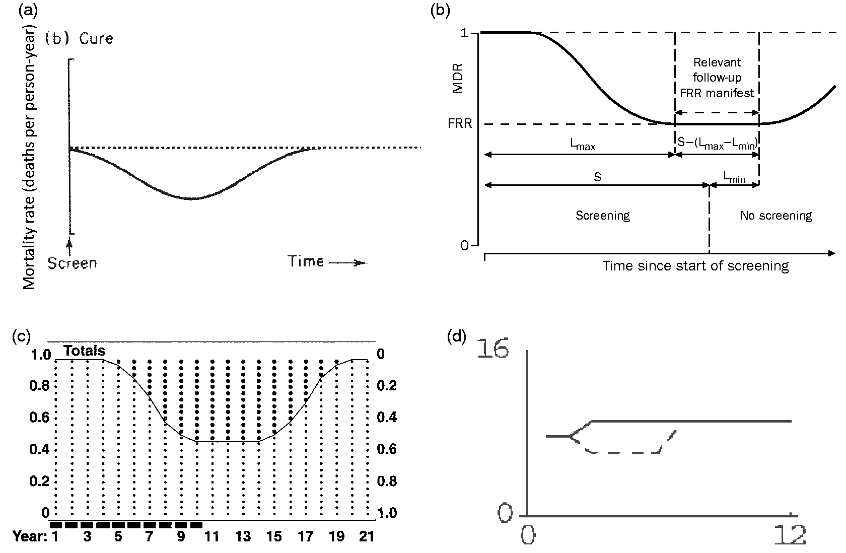
Much of the statistical work that has addressed this non-proportional hazards time pattern has focused on statistical tests applied to data from screening trials, and thus on maximizing statistical power7,8 dealing with the non-proportionality 9 , and selecting the optimal time at which the analysis of trial data should be carried out. 10 The data analysis in each actual trial tested a regimen-specific null hypothesis over some (un-predetermined) follow-up period: “does the amount and spacing of screening used in this trial have a non-zero impact on cancer mortality?” There has been much less focus on deducing the impact of a sustained screening programme.
2 Distinction between nadir in a trial and asymptote in a programme
Trial nadir and programme asymptote
Our focus is on identifying the asymptote of the rate ratio curve, as it represents the sustained reduction that could be expected from a screening programme. In the following, we describe how it is possible – but only in some instances – to estimate the programme asymptote from trial data.
Figure 3 shows the distinctive
patterns produced by a trial of 3 annual screenings versus by a programme of 20 annual
screenings. If each round of screening reduces mortality over 5 future years, then three
rounds would produce 3 waves of such reductions. The affected time window spans over a
total of 7 years, with a maximum reduction of 35% in year 6. In contrast, a programme of
20 screenings would produce 20 such waves, affecting many more years, with a sustained
reduction of 46% for 16 years, much longer and deeper than the width and the maximum depth
of the reductions seen in a trial. As is seen by comparing panels (a) and (b), the nadir
seen in a trial usually underestimates the asymptote in a programme. However, even if all
that was required was to measure the nadir carefully by, for example, smoothing
11
to avoid overestimation
resulting from the yearly statistical fluctuations, few trials have provided yearly data
that might allow this to be done. Instead, the universal practice is to report an averaged
reduction, computed over the entire follow-up time of the trial. Because this average
includes the almost-zero reductions outside the affected time window, it is even smaller
than the nadir, and thus an even greater underestimate of the programme asymptote of
interest. The 35% maximal mortality reduction produced by a
(hypothetical) trial of 3 annual screenings (a) does not necessarily reach the 46%
asymptote produced by a programme of 20 annual screenings (b), particularly if the
impact of each round is spread over more than 3 years. Shown in (a) is a
hypothetical trial of 3 annual rounds of cancer screening
(S1, S2, S3) compared with no screening. The
depth of the white rectangle in each year represents the percentage mortality
reduction, relative to an unscreened group, for the year shown on the horizontal
axis. Annual mortality reductions produced by screening only begin to be expressed
in year three (when the first effect of S1 is discernible); they are
greater in years 4 and 5, reaching a maximum of 35% in year 6 (when the combined
effect of S1, S2 and S3, denoted by ‘1’ , ‘2’ and
‘3’ respectively, is maximal); in year 7 the combined effects begin to wear off, and
the mortality in the screening arm begins to revert to that in the non-screening
arm; in year 9, the last effect of S3 is discernible. Thus the maximum
reduction is 35% and it would have been greater than if screening had not been
discontinued at year three. By contrast the average effect of
screening over the 13 years of observation (the metric used by task forces) would be
12%. Shown in (b) is a hypothetical screening programme with annual
screening beginning at age 50 and continuing until age 69, compared with no
screening. Again, the depth of the white rectangle represents the percentage
mortality reduction for the age shown on the horizontal axis. The mortality
reduction reaches 46% at age 56 and is maintained at that level for many age-bins –
until three years after the last screen when it starts to decrease
again.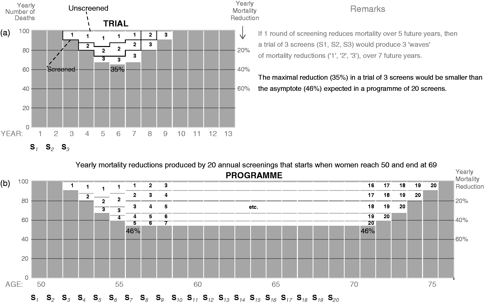
Lung cancer deaths in the NLST report.
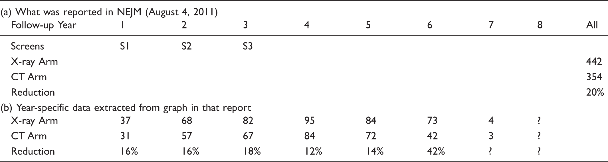
The additional numbers of cancer deaths in years 7 and 8 were unknown at the time of the report, because the causes of the deaths that occurred in these latter years had not all been adjudicated by the time the overall mortality reduction became statistically significant. This is a striking example of the distinction between getting a statistical significant result with just 3 screens, and providing evidence on what a screening programme (of possibly many more screens) would achieve.
The importance of using time-specific rates to pursue the asymptote of the curve was also highlighted in a recent review of screening trials in colon and prostate cancer. Whereas the overall reduction in the largest colon trial been reported to be 20%, the re-analysis, which took account of the timing of, and interruptions in, screening, found that an uninterrupted programme would yield reductions with an asymptote of 40%. 3 In screening trials for prostate cancer, where the time lag between screening and when the mortality deficits manifest are even longer, the deficits produced by the first screen would not be expected for at least six years; however the majority of the follow-up has only extended to about year 11 in the European Randomized Study of Screening for Prostate Cancer (ERSPC). 13 A re-analysis 14 showed that the reductions only began in year 7, and reached an asymptote of approximately 50% by year 12. One commentator 15 put it well: “perhaps a better summary of the European trial result is not the 20% overall reduction in prostate cancer mortality, but the combination of no reduction in the first seven or so years and a reduction of about 50% after 10 years”.
Several task forces have examined screening programmes for breast, lung, colon and prostate cancers. Although their stated purpose was to estimate what a sustained programme would do, all of the meta-analyses they used merely averaged the overall reductions seen in different trials. Thus they all greatly underestimated the asymptotes that would characterize the programmes they considered. 4
A few authors have explicitly dealt with the delay, either by using the hazard ratio from a certain time point onwards 16 , or (in those trials with a sufficiently long duration of screening), by ‘letting the data speak for themselves’ as to when the asymptote begins.2,13
An alternative metric
An alternative approach, that indirectly addresses the asymptote and directly acknowledges the time-pattern of the reductions produced by a limited number of rounds of screening, is to examine the mortality impact only in cancers diagnosed during the screening period. This avoids the dilution, which Baker 5 refers to as “post screening noise”, described above: cancers that arise long after the screening is discontinued could not have been affected by the screening carried out in the trial. In one version 17 of this alternative approach, where the cumulative incidence of cancers deaths - in those diagnosed in this screening period - in the two study arms are compared, it is assumed that there is no over-diagnosis in the screening arm. The other version 18 avoids having to make this assumption by using the number of cancers that were diagnosed in the non-screening arm during the screening period. The efficacy of the 3 rounds of CT screening is then determined by calculating the `deficit’ of (442-354 =) 88 cancer deaths, and expressing this 88 as a percentage, not of 442, but of the number that could possibly have been helped by screening (the 88 who were, and the xxx whose cancers, despite being diagnosed in the screening period in the screening arm, proved fatal nevertheless). Unfortunately, as of the time of writing, this number xxx is not known.
The approaches described above do not allow projections to be made for a programme that uses a different spacing of screening examinations than was used in a trial. We therefore here describe some (necessarily-model-based) that do. This round-by-round approach also makes it possible to deal with trials in which the nadir may not have reached the asymptote.
3. Projecting the reduction patterns that would be produced by different regimens from those used in trials
Approaches
Because a trial usually does not contain sufficient rounds of screening, the nadir observed in it would underestimate the asymptote expected in a sustained programme with the same spacing of screenings. Thus, modeling assumptions are required to extrapolate from a trial of say 3 annual screens to a programme with say 20 annual screens. The ‘round by round approach’ we have described in Figure 3 can also be immediately applied to programmes with different durations and spacings (eg. 20 annual screens versus 10 biennial screens).
Several projections of the mortality reductions due to cancer screening have been based on extensive modeling of the natural histories of cancers and how their progress is altered by earlier detection and therapy. Many of these efforts19–21 have also quantified the associated costs and use very sophisticated simulation modeling to examine the impact of prevention, screening, and treatment on cancer incidence and mortality at the population level. These approaches usually require a very large number of parameter inputs, obtained from diverse data sources (such as trials, registries and surveys).
We first illustrate a round-by-round approach, using the model proposed by Hu and
Zelen.
10
Previously, it has mostly been used for planning early-detection trials, including the
recent NLST, where the yearly numbers were aggregated for the power calculation for the
interim and ultimate statistical tests performed during and at the end of the trial. We
use it here to generate and display the rate ratio curve proposed in Section 1, to show
the projected timing, magnitude and duration of the yearly reductions in a
programme (the yearly numbers that the software aggregates for power
calculations do not appear to have been previously used for this purpose). Hu and Zelen
model the mortality in each year under the screening and no-screening scenarios via a
total of seven parameters (see Figure
4) quantifying the sensitivity of the screening test, the natural (and altered)
course of cancer from initiation to normal clinical diagnosis and post clinical diagnosis.
A
35-year projection of lung cancer mortality reductions for a programme of (a) 20
annual and (b) 10 biennial screenings, based on the same Hu-Zelen model used to plan
the NLST trial but with the 7 indicated input parameters (see text re the
sensitivity and survival inputs), together with the associated (almost-bathtub
shaped) rate ratio curves. The comparison is between screening with low-dose CT
screening and Chest X-Ray (shown to be virtually ineffective in the PLCO trial). The
‘excess’ deaths after years 25 are a consequence of the exponential survival
assumption in the Hu-Zelen model, in which cancer deaths are merely postponed, not
averted – similar to the pattern shown in Figure 2-5(a) in Morrison’s textbook.
Newer programme projections will be made once we have extracted parameter values
from the NLST data.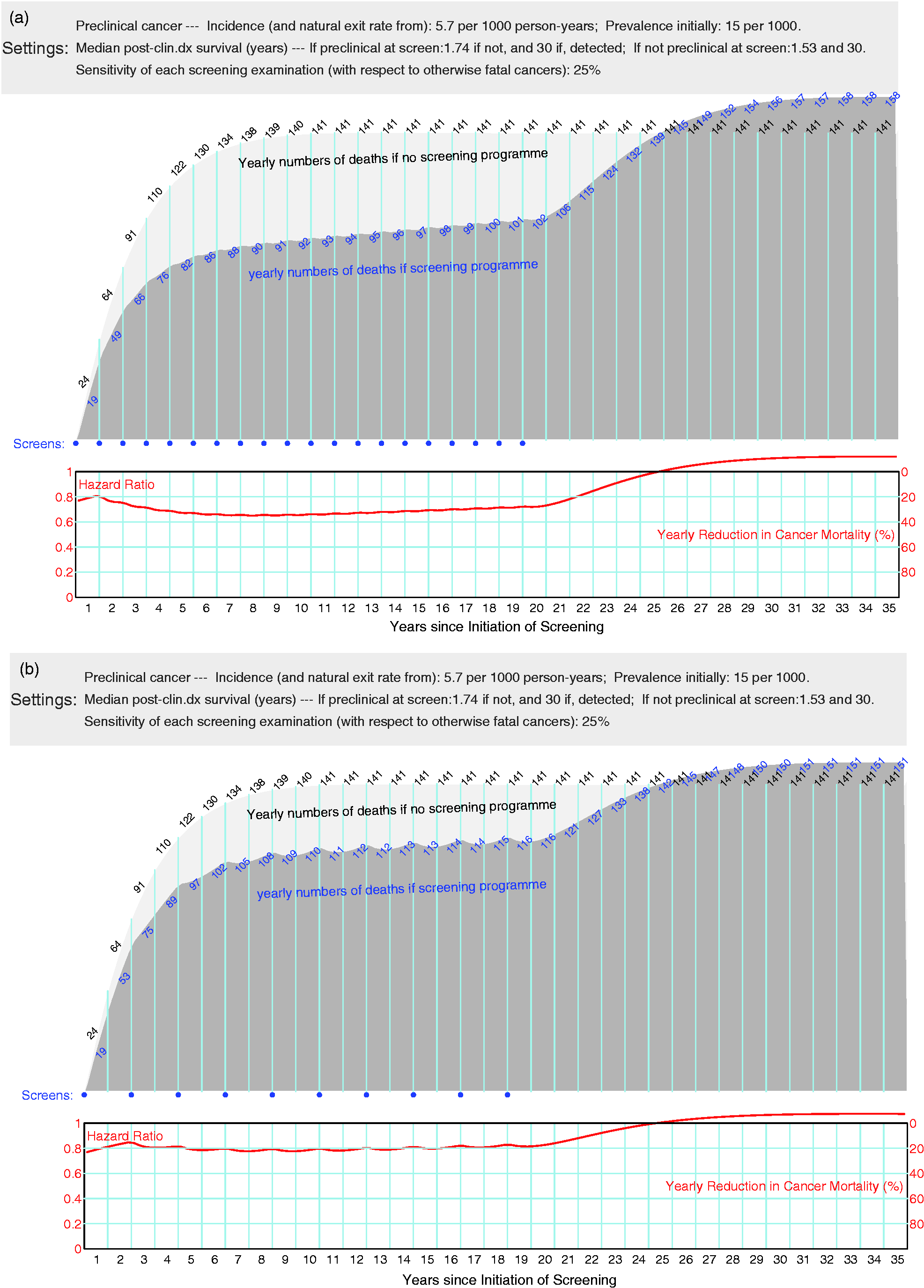
Illustration
As sufficient information to fit new parameter values has not yet been extracted from the completed NLST, we will use some modifications of the input values 22 used to plan the trial. Rather than use the FORTRAN software the trial statisticians used to implement the Hu-Zelen integrals, we re-programmed them in R. The only modifications we made were to two of the input parameters, to better represent how the cancer deaths are averted. In the planning, the authors assumed the ‘average’ CT sensitivity would be 85%, and that those whose cancers were detected by screening would have their (counterfactual) post-clinical-diagnosis survival altered from an exponential distribution with a median 1.53 or 1.74 years to one where the median was 2.42 or 2.21 years: (the planning calculations assumed that all would eventually die of their cancer; moreover, there was no possibility of a ‘cure’, unless by a ‘cure’ one means that one dies of another cause). Instead, in light of the very rapid progression of many lung cancers, and the possibility of over-diagnosis, we assumed that the ‘real’ sensitivity was much less, and that the possibility of cure (rather than a very short extension of a few months of life) was confined to subgroup of screen-detected cancers; the remainder, even if detected by screening, would continue to have virtually the same mortality rates as their counterparts who were not screened. Thus, we set the ‘sensitivity’ at 25% rather than 85%, and the median survival of 30 years (‘cure’) for those whose otherwise fatal cancers were found at a curable stage.
Figure 4(a) shows the resulting 35-year projection for a programme of 20 annual screenings. With the exception of the slightly unrealistic (but numerically inconsequential) pattern at the front end (see below), the rate ratio curve, and its complement the reduction curve, resemble the anticipated bathtub-shape presented in Figure 1. The curve stays close constant for the middle part where there was sustained screening, and it gradually tails off after screening was stopped. The ‘excess’ deaths after years 25 are a consequence of the assumed exponential survival model in which cancer deaths are merely delayed, not averted – in keeping with the corresponding pattern shown in version (b) of the Figure in Morrison’s textbook.
Figure 4(b) shows the projection for a biennial programme; it is a little shallower than the annual one, but the reductions persist for almost the same duration. The oscillations in the ‘round by round’ waves are more prominent than in (a), and reflect the local effects of variations in the progression rates of different cancers together with the intra-individual variability in their stages at each examination time. The considerably smaller morality reductions than in (a) emphasize the fact that two year screening intervals allow many more lung cancers to progress to the incurable stage in the interim.
Possible reasons why the early portion of the projected curve does not show the anticipated time lag more clearly may include (i) the numbers of cancer-specific deaths are expected to be very small in the first few years, which lead to large uncertainty in the early portion of the rate ratio curve; (ii) the exponential form, assumed for the sojourn time distribution, does not take into account the time lag between screenings and their induced mortality reductions, (iii) the assumption of independence between an individual’s sojourn time and their post-clinical diagnosis survival time: we would expect a strong correlation, that is, a relatively fast-growing cancer would be aggressive both pre- and post-detection; and (iv) the mortality rates do not explicitly accommodate cures from cancer nor deaths from other causes.
In order to deal with these front-end and back-end issues, considerably more refinements would need to be incorporated into the model, such as stage-specific sensitivities, transition rates, and survival distributions, as well as age-specific competing risks. While Zelen and colleagues, and other CISNET investigators, have indeed incorporated such refinements, they now face the reality of having to deal with the over-diagnosis that accompanies the newer screening tools, and the added model complexity and uncertainty. Instead, we are currently exploring a minimalist model that focuses only on the mortality reductions.
Conclusion
Unlike therapeutic trials in patients, cancer screening trials in asymptomatic persons generate mortality reductions that can only manifest several years after the onset of screening. The often reported single-number cumulative mortality reduction, in either a trial or a meta-analysis of trials, is of limited use in projecting the timing, duration and magnitude of the mortality reductions that would be expected from a sustained screening programme, of longer duration and possibly with a different screening regimen.
Instead, we propose using a rate ratio curve, and its complement, the mortality reduction curve, to address the mortality impact (timing, magnitude, and duration) of a screening programme. This curve is easy to interpret, as it shows when reductions begin, how big they are, and how long they last. We illustrate, using an existing model, how such rate ratio curves could be computed and how it is possible to quantitatively compare the impact of different screening regimens over the appropriate time-window.
Our message is two-fold: we (1) recommend against using one-number summaries to deduce the yearly mortality reductions expected from a sustained screening programme, and (2) call on trialists to report necessary time-specific mortality data to allow the appropriate computation of rate ratio curves that allow the mortality impacts of different screening programmes to be compared over the appropriate time horizon.
Footnotes
Funding
This work was funded by the Canadian Institutes for Health Research.