Sage Journals: Discover world-class research

Abstract

The proposed research explores Multi-Walled Carbon Nanotube’s (MWCNT’s) effect on the mechanical buckling behavior of glass fiber-enhanced thermosetting composites using UTM and the load vs displacement curve is plotted. Using the inflection point method, the critical buckling load is obtained from the load vs displacement curve for beams with three different volume fractions of MWCNT. The nonlinear finite element method is used to numerically obtain the load vs deflection curve and the numerical results are compared with the experimental results, and a close match is found with the experimental results. It is observed that the nonlinearity associated with the structure can significantly reduce the critical buckling load. The critical buckling load is found to increase and reported a 27.4% increase in buckling load with 0.3 wt.% of MWCNT which could be accounted for the increase in flexural modulus of the material.

Keywords

MWCNT composite linear buckling analysis nonlinear buckling analysis experimental analysis polymer composite

Introduction

Composites are materials consisting of two or more physically or chemically distinct phases combined macroscopically to yield a useful material. These materials have superior properties compared to an individual material. The synthesis, processing, and future application of polymer nanocomposites have drawn academic and industrial attention and interest due to their superior properties such as higher rigidity, higher strength, and excellent chemical resistance.¹ To improve the properties of the material, the polymer composites are supplemented with nanofiller materials. The incorporation of CNTs into a polymer matrix along with fiber reinforcements to produce hybrid composites have attracted significant attention in recent years. Nanofibers, metal nanoparticles, and nanoclays are commonly used nanofiller materials. The discovery of Carbon nanotubes (CNTs)² has stimulated intense research on its structure, properties and application. The exceptional properties of CNTs such as high thermal, electrical, and mechanical properties complimented by its low density has led to their use as filler material in nanocomposites.^3,4 As CNT possesses a higher area to volume ratio, it creates more interface with the epoxy matrix thus increasing the load-carrying capacity of the nanocomposite, which in turn increases the strength of the composite. The CNT-polymer composites have wide applications ranging from ultra-strong materials for bulletproof vests, flexible displays to electronic paper.⁵ Adding CNT to composites improve the mechanical property, decrease weight and act as heat conductor.⁶ Various methods such as compression molding, Resin Transfer Molding (RTM), Vacuum-Assisted Resin Transfer Molding (VARTM)^7–11 or wet hand lay-up process^12–14 are used for the manufacturing of nanocomposites. Compression molding is one of the most common processing technique to fabricate plastic and polymer composite products. Fiber-reinforced thermoplastic resins such as glass fiber reinforced thermoplastics (GMT) and long fiber reinforced thermoplastics (LFT) are attracting interest from the automotive industry. Their excellent toughness and recycling possibility led to a wide application of thermoplastic compression molding for the fabrication of nanocomposites. Advantages of compression-molded parts, such as exhibiting better dimensional stability along with the interior and exterior surface finish make this technique as one of the most promising methods for fabrication of polymer nanocomposite.¹⁵ Buckling is an instability that leads to structural elastic failure in which it is unable to take on the additional load. Buckling occurs after a certain point when a structure is subjected to compressive load and is characterized by a sudden sideways deflection.^16,17 The current research focuses on the influence of volume fraction of MWCNT’s on beam buckling behavior and the numerical results obtained using ANSYS have been validated with the experimental results.

Experimental details

Fabrication of nanocomposites

Materials

The nanocomposite specimen manufactured using compression molding consists of three constituents, the matrix, fiber, and the nanofiller. The matrix phase is Bisphenol A diglycidyl ether (DGEBA) epoxy with hardener Triethylenetetraamine (TETA) hardener available in their trade names Lapox L-12 and Hardener 301. The epoxy to hardener weight ratio is taken as 10:1.¹⁸ The glass fibers used are woven E-glass roving (360 GSM) fibers. To obtain the necessary thickness, 16 layers of glass fibers are stacked one over the other. The nanofiller used in this analysis is MWCNT with an average diameter of approximately 10–15 nm. It has a purity of 99% with an approximate length of 15 μm.

Fabrication of mold

The mold base of thickness $0.008 m$ is made using cast iron. The frame is made of mild steel which has good machinability to easily produce the cavity for the composite specimen. The frame and the base are welded together to prevent slippage while loading in the compression molding press. The mold is used to fabricate a composite having the dimensions of 0.24 m × 0.24 m × 0.004 m. To improve the composite surface finish, the polymer sheet is folded in cuboid shape and put within the mold. The use of these sheets made the removal of the nanocomposite from the mold easily achievable. Mansion wax is added to improve the consistency of the specimen so that any leakage of the adhesive epoxy does not bind on to the mold. The edges are supplemented with extra wax to facilitate the easy removal of the composite.

Fabrication of (glass epoxy) GE composite

The fabricated mold has a cavity depth of $0.004 m$ to yield a composite plate of dimension 0.24 m × 0.24 m × 0.004 m. Each layer of woven roving glass fiber mat is placed one over the other. Within the composite, the fraction of E-glass fiber and epoxy is held at a weight ratio of 60:40. Based on the estimates, it is found that it takes 0.22 kg of epoxy with a 0.022 kg hardener to fill the mold cavity and the epoxy and hardener are mixed in the ratio of 10:1 as per the datasheet. The ensuing suspension is stirred for a specific duration to ensure uniform distribution of hardener in epoxy, which leads to air bubbles formation. The thus formed air bubbles are removed from the suspension, to prevent the creation of void spaces in the formed composite. The bubbles are removed from the suspension by desiccating at 700 mm of Hg for 2 min. If care is not taken to eliminate these air bubbles, void spaces in the final cured composite can seriously affect the mechanical properties of the composite and can act as stress concentration inside the material. GE composite is manufactured using a hand lay-up process in which the epoxy is uniformly poured over the surface of the mold, backed by adding glass fiber on top of the epoxy poured in. Similarly, 16 layers of glass fiber are stacked with intermediate epoxy filling and followed by a hot press in a compression molding system (Santosh SHP-50) at a temperature of 80°C with a pressure gauge reading of $2 \times 10^{6} {N/m}^{2}$ for 1 hour. The parameters for curing in the hot press is selected based on the manufacturer’s catalog.

Fabrication of MWCNT-GE nanocomposite

The measured amount of epoxy is taken in a beaker and different weight fractions of MWCNT are added to the same. The epoxy/MWCNT suspension is sonicated in Vibra-Cell VCX 750 sonicator at a frequency of 20 kHz, a pulse time of 7 s, and a rest time of 3 s for a total duration of 1 hour. The sonication process allows MWCNT to be well dispersed in epoxy resin. The sonication process triggers the formation of air bubbles. The hardener is added to the suspension after the sonication process and is stirred for uniform hardener mixing resulting in further bubble formation. Entrapped air bubbles can result as void spaces in the finished nanocomposite and the desiccator removes them. The layup of glass fiber is similar to the manufacture of GE composite. The schematic of the fabrication technique is as shown in Figure 1.

Figure 1.

Fabrication of nanocomposite: (a) mixing of epoxy and MWCNT in their respective proportion, (b) sonication process using the probe sonicator, (c) desiccation, (d) hand lay-up of first layer, (e) uniform distribution of mixture on the glass fiber, (f) hand lay-up of 16 layers of epoxy + MWCNT mixture, (g) compression mold pressing, and (h) separation of the specimen from the mold.

Material characterization

The molded composite plates are cut using hand cutters into ASTM standard specimens to obtain mechanical properties such as flexural modulus and flexural strength. Beam specimen with $0.13 m$ length and $0.03 m$ width is used and a three-point bending test is carried out as per ASTM D790. Zwick Roell, Z020 UTM is used for testing purposes. A bar of rectangular cross-section is rested on the two supports and is loaded utilizing a loading nose midway between the supports. For the flexural test, the specimen is subjected to a preload of $0.1 MPa,$ and the displacement is given at a rate of 2 mm/min. The loading in the specimen is measured using a 20 kN load cell. The specimen is deflected until rupture occurs in the outer surface of the test specimen or until a maximum strain of 5% is reached, whichever occurs first.

A critical defect that is likely to occur in the matrix is voids i.e. its porosity. To improve the interlaminar shear strength, the porosity in the matrix of the nanocomposite should be significantly low.¹⁹ Void content in the fabricated nanocomposite is calculated by comparing experimental and theoretical densities calculated based on the rule of mixture. The densities of glass fiber and epoxy resin is $2550 {kg/m}^{3}$ and $16000 {kg/m}^{3}$ , respectively. The estimated theoretical density using the rule of mixture is found using the formula as shown in equation (1)²⁰

ρ_{c} = ρ_{m} V_{m} + ρ_{r} V_{r}

where, ρ designates the density and V represents volume fraction, with the subscripts c, m, and r denoting the composite, matrix and reinforcement, respectively. The experimental density test is carried out as per ASTM D 792-13. The density of the composite is determined by measuring the volume of water displaced by the Archimedes principle as the composite is put into water. The experimental densities of the composites are noted down. The void content is found using the following relation (equation (2))

Void (%) = \frac{ρ^{th} - ρ^{exp}}{ρ^{th}} \times 100

X-Ray powder Diffraction (XRD) technique to identify the phase identification of a crystalline material present in the composite have been utilized and provides information on unit cell dimensions. The XRD analysis is done using the X’PERT-PRO X-ray diffraction system with the PW3050/60 console (goniometer). The high voltage generator is set to 40 kV and 30 mA current. The anode was made of copper and the minimum step size 2θ is set as 0:001. The scan was done from 5° to 50°.²¹ The intensity (cps) v/s angle (2θ) is plotted using Origin® software. The marker is set at the highest peak in the plot and a Gauss fit is applied to derive the full-width at half-maximum (FWHM) value and the angle at which the highest first-order peak is located. The y-axis marker is used to derive the intensity at that point. The crystallite size is found using the Scherrer equation²² as shown in equation (3)

D = \frac{K λ}{β cos θ}

where, D is the crystallite size in nm. The value of K is 0.9 known as Scherrer constant, $λ$ is the wavelength of the X-ray source, $β$ is the FWHM in radians and $θ$ is the peak position in radians.

Buckling analysis

Analytical analysis

When a short column or strut is subjected to a gradually increasing compressive load, it will result in the crushing of the structure. The stress generated during this crushing phenomenon is P/A, and this happens when the load, P applied is purely centrally through the center of gravity of the cross-section, A or P/A + Pey/I when the load is off-center. Yet consider a situation where the column is long and the compressive strain on the structure tends to bend out sideways at a much smaller strain than is required to crush the material. It is shown that the column fails by bending near the middle depending upon the boundary conditions. According to Euler, the maximum compressive stresses that occurred during buckling should remain within the proportional limit of the material, when assumed the column to be slender.²³ The Euler’s buckling formula is given in equation (4)

P_{c r} = \frac{π^{2} E I}{{(0.7 L)}^{2}}

where, P_cr is the maximum force, E is the modulus of elasticity, I is the area moment of inertia, L is the unsupported length of the column and K = 0.7 represents the column effective length factor for the boundary condition analyzed.

Numerical analysis

Linear buckling analysis

Eigenvalue linear buckling is used to calculate the critical load of ideal structures and is comparable with the Euler buckling load. This analysis predicts the theoretical buckling strength of an ideal elastic structure. The structure is assumed as most ideal with homogenous composition and zero imperfections. The plastic behavior of the material is not considered and the stiffness matrix is zero after the bifurcation point. This method corresponds to the analytic approach to elastic buckling analysis. The governing finite element equation for the analysis is discussed assuming [K] as the stiffness matrix and is given by equation (5)

[K] = \int {[B]}^{T} [D] [B] d V

where, [B] is the matrix defined using the derivatives of the nodal shape functions. The strain vector {e} is given by equation (6)

{e} = [B] {u}

where, {u} is the displacement vector. The change in displacement vector {u} is assumed negligible, thus {u} is a constant. [D] is the stress displacement matrix that gets altered according to the changes in properties like Young’s modulus, Poisson’s ratio, etc. The volumetric integration of this constant displacement gives a constant [K] matrix. The stiffness equation of the system is given by equation (7)

[K] {u} = {F}

{F} represents the force vector that includes the boundary forces, weight, etc. For satisfying the equation [K] should be singular as shown in equation (8)

| [K] - λ [K_{g}] | = 0

[ $K_{g}]$ is the geometric stiffness matrix or linearly perturbed stress stiffening matrix and is given by equation (9)

[K_{g}] = \int {[B_{g}]}^{T} [D] [B_{g}] d V

The eigenvalue $λ$ is calculated and the lowest one is selected. In most symmetrical structures the first mode of buckling constitutes the lowest eigenvalue, $λ$ . The close approximation of the eigenvalue buckling load is used as the force applied during the nonlinear buckling analysis.

Nonlinear buckling analysis

The nonlinearity in the structure is unaccounted during the linear eigenvalue buckling analysis. A slender structure in practice may, therefore, have some form of nonlinearity that needs to be accounted for. Thus, a nonlinear buckling analysis is performed to consider the imperfections and nonlinearity and a load vs deflection curve is plotted. In the nonlinear buckling analysis, the irregularities and imperfections of a structure are taken into account. The imperfections are either due to geometric imperfections or material imperfection. Geometric imperfections include curvy nature, lack of parallel surfaces, initial perturbations, etc. Material imperfections are due to voids, internal defects, lattice distortion, etc. To account for these defects partial differential equations (PDE) are utilized in the nonlinear buckling analysis. More coefficients are added to the matrices that make it more complicated and results in truncation and round off errors. In a nonlinear buckling analysis, stiffness matrix [K] is assumed to be a function of displacement {u} as shown in equation (10)

[K] = f ({u})

Due to this reason, the stiffness matrix found by volumetric integration is not valid for the analysis. Moreover, the displacement vector is further dependent on the previous matrix i.e. ${u} \leftrightarrow [k (u_{0})]$ . An iterative approach is used to solve this interdependency. It is assumed that ${u} = {u_{0}} = 0$ . The value of $[k (u_{0})]$ is calculated and the stiffness equation is solved by equation (11)

[k (u_{0})] . {u_{1}} = {f}

The above equation is not exact as $[k (u_{1})] . {u_{1}} - {f} \neq 0$ , so it is iterated till equation (12)

[k (u_{n})] . {u_{n}} - {f} \approx 0

A nonlinear approach involves two methods for solving the problem. LBMI (Linear Buckling Mode-shape Imperfection) method²⁴ and the SPLI (Single Perturbation Load Imperfection) method.²⁵ In the LBMI method, the axially symmetric mode shapes generated using the linear buckling analysis (eigenvalue buckling) is used as the initial geometry for nonlinear analysis. In the SPLI method, a local distortion or local perturbation is generated in the structure by applying a lateral load and buckling was continued by applying an axial load. They found that after reaching a certain lateral load, the structure will lose its sensitivity to lateral load and the corresponding axial load to this lateral load is assigned as the critical buckling load.²⁶ The LBMI method is proven to give closer approximate solutions to the experiments and is used to solve the presented problem.

The critical buckling loads obtained using linear buckling analysis are over predicted values. The nonlinear buckling analysis is performed in tandem with the static structural and eigenvalue buckling analysis. Static structural analysis is performed to obtain the geometric stiffness matrix and is coupled to linear buckling analysis to obtain the critical buckling load and the fundamental buckling mode shapes. Large displacements for both static structural and eigenvalue buckling analysis are neglected, whereas they are considered for the nonlinear analysis performed. The results of linear buckling with first mode shape with scaling factor is set as initial geometry for nonlinear buckling analysis. A beam of a constant cross-sectional area of 0.01 × 0.004 m² (breadth × height) and a gauge length of 0.12 m is modeled using ANSYS Design Modeler with both ends fixed support in ANSYS®. The actual buckling load can be estimated from the load vs displacement curve of nonlinear buckling analysis using inflection point method.

Experimental analysis

The numerical analysis provides us the load corresponding to which buckling in specimens occurs. To carry out experimental analysis, composite column specimens of dimension 0.24 m × 0.01 m × 0.004 m (length × breadth × height) are used. The buckling test is carried out in Heico HL0693 UTM, where the composite specimens are inserted in jaws with a gauge length of 0.12 m as shown in Figure 2. A load cell of 25 kN is selected based on the results obtained from the numerical analysis. The end jaws are tightened and are assumed as a fixed boundary condition at both ends permitting one-dimensional translation at the moving jaw. Axial displacement is given in the vertical direction (movable jaw), at the rate of 2 mm/min. The specimens are loaded up to breakage and the load vs displacement graph is plotted for three specimens of 0 wt.% MWCNT-GE, 0.1 wt.% MWCNT-GE and 0.3 wt.% MWCNT-GE.

Figure 2.

Schematic representation and experimental setup of the specimen held in Heico HL0693 UTM for the buckling test.

Results and discussion

X-ray diffraction

The crystallite size and the presence of MWCNT are verified using XRD analysis by analyzing the peaks obtained in the plot between intensity vs degree of diffraction as shown in Figure 3. The presence of peaks in the plot obtained helps to identify the presence of carbon in the specimen tested.²¹ The crystallite size of the MWCNT is found using Scherrer equation.²² Figure 3 shows that the first peak of diffraction occurs at $2 θ = 25.68 ° .$ The result obtained is similar to the plot obtained by Jia-Jia et al.²⁷ and Sankal and Kaynak²¹ found for MWCNT. The plot rules out the presence of any impurities like Sulphur on the MWCNT which would alter from the present peak angle. Using the Scherrer’s equation, the first order peak corresponds to the MWCNT having d-spacing of 5.449 Å. The highest peak occurs at an intensity of 1932 cps which indicates the presence of s-MWCNT i.e. aminosilanized MWCNT. This range of intensity is due to the absorption coefficient of the elements present in aminosilane groups of s-MWCNT.²¹ The crystal structure of s-MWCNT is identical to that of MWCNTs.

Figure 3.

X-ray diffraction of MWCNT.

Density test

The volume fraction of the matrix, reinforcement and the filler material are calculated. Since the fiber reinforcement volume remains constant, the volume fraction of MWCNT (in wt.%) is plotted as shown in Figure 4.

Figure 4.

The fiber volume fraction of the nanocomposite specimens prepared.

The density test resulted in acquiring knowledge about the void content in the nanocomposite. These voids may be due to the manufacturing defects that occur due to blow holes during the exothermic reaction between the epoxy and the hardener and also due to the bubble formation during the stirring and sonication operation. The desiccation of the mixture after sonication reduces the air bubbles formed up to a limit. The result of the void test using the rule of the mixture is shown in Table 1.

Table 1.

Density values of nanocomposites fabricated.

Specimen (MWCNT-GE)	Experimental density, ${kg/m}^{3}$	Theoretical density, ${kg/m}^{3}$	Variation, %
0 wt.%	1701.34	1729.21	1.61
0.1 wt.%	1703.70	1729.44	1.49
0.3 wt.%	1712.80	1729.89	0.99

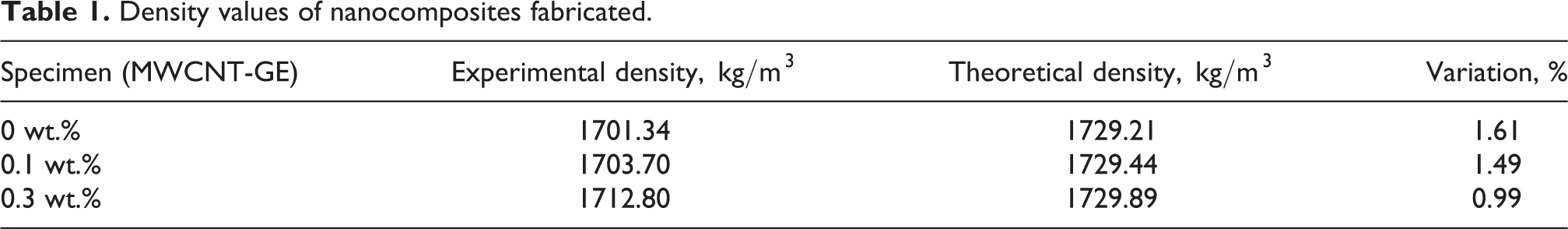
Table 1 shows that as the wt.% of MWCNT increases, the void presence reduces that results in a higher density of MWCNT-GE nanocomposite. This can be accounted for a decrease in viscosity due to the increase in temperature during the sonication process,²⁸ leading to its easy flow in the mold cavity during the compression molding process. Also, nanoparticles tend to act as fillers in the voids, which in turn reduces the void content of the nanocomposites²⁹ by 8.3% and 63.1% with the addition of 0.1 wt.% and 0.3 wt.% MWCNT respectively.

Flexural test

The specimens were loaded at a rate of 2 mm/min for a three-point bending test which resulted in the specimens bending. After the three-point bending test, it was seen that at about 1.5% to 2.0% deformation, the specimens encountered its first breakage as shown in Figure 5 and 0 wt.% MWCNT (GE-composite) had the highest flexural strength. Since the nanotubes may have formed a cluster or agglomerate among themselves, as the MWCNT content is increased the flexural strength decreases (Figure 6). This results in a filler–filler interaction and lower interfacial properties promoting an internal shear delamination.³⁰ The nanotubes should have occupied the voids in the nanocomposites,²⁹ which results in few points of agglomeration of MWCNT and they act as points of stress concentrations, thus providing sites for crack initiation.³⁰

Figure 5.

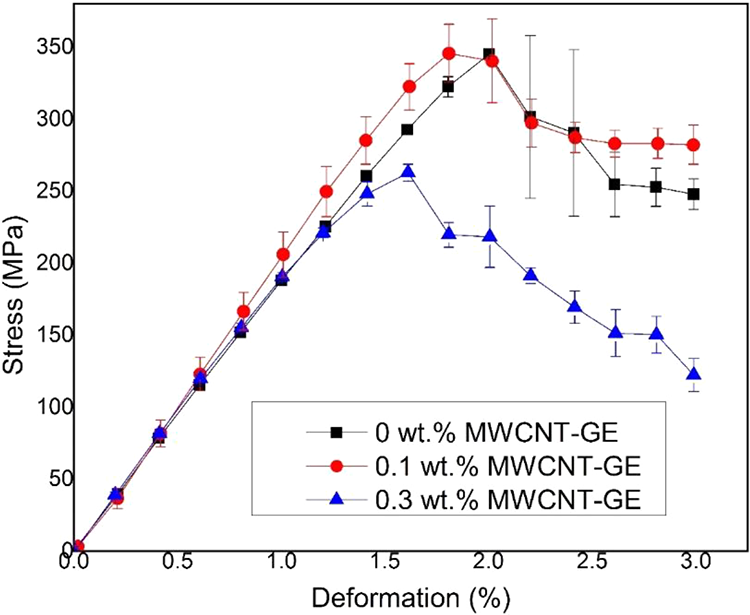
Stress vs deformation curve in a flexural test.

Figure 6.

(a) Flexural strength and (b) flexural modulus of the MWCNT-GE composite specimens.

On the contrary, the flexural modulus is seen to increase with the addition of MWCNT wt.% as shown in Figure 6. Hence, this proved that MWCNT takes up the load and the increase in contact area has helped the MWCNT-GE nanocomposite to withstand more load in the elastic region. Due to the presence of aminosilanised MWCNT (s-MWCNTs), leads to the formation of either hydrogen bonding or covalent bonding at the interface. Hence, the load transfer mechanism from the matrix to the reinforcement works efficiently, which allows it to withstand the compressive load.

Buckling test

Analytical solution

The Euler buckling load is calculated using the Euler buckling formula and the results are tabulated in Table 2.

Table 2.

Comparison between different buckling loads.

Sample (MWCNT-GE)	Euler equation, kN	Eigenvalue, kN	LBMI, kN	Experiment, kN	Stiffness, kN/m
0 wt.%	2.88	2.87	1.32	1.35	940
0.1 wt.%	2.89	2.89	1.57	1.55	960
0.3 wt.%	2.97	2.93	1.69	1.72	1040

Numerical analysis

The Poissons’ ratio of the composite specimens are assumed as 0.28.²⁶ The flexural modulus obtained from the three-point bending test is given as an input to the numerical analysis to solve linear and nonlinear buckling analysis. From mesh convergence study, it is found that the solution converges at 8309th node and 1600 elements. The directional deformation is seen to converge with 40 number of divisions along the gauge length. This means that it corresponds to the minimum number of divisions (keeping the number of divisions along the length and height constant) for assured convergence of the solution. Quadratic Hexahedron is selected as an element type for the beam, as it represented a simple structured grid with a tessellation of quadrilateral in 3D. The beam is divided into a finite number of divisions as 10 divisions along the length (X-axis), 4 divisions along the width (Z-axis) and that of height were 40 divisions (Y-axis).

Linear buckling analysis

From the eigenvalue buckling analysis carried out using ANSYS®, the load multiplier for each specimen were obtained. Hence, the eigenvalue buckling load is calculated and tabulated in Table 2. This eigenvalue buckling loads are applied as load in the nonlinear analysis. The nodal displacement solution for the fundamental buckling mode shape is extracted from the linear buckling analysis and using a scale factor to the mode shape, the initial geometry for the nonlinear buckling is modeled.

Nonlinear buckling analysis

The scale factor is selected as 5, 5.2 and 5.5 for 0 wt.% MWCNT, 0.1 wt.% MWCNT and 0.3 wt.% MWCNT to accommodate the nonlinearities and imperfections that may occur due to the geometric, material, and loading variations.

Physically scale factor refers to the fraction discontinuities in a material. It implies that lesser the discontinuities the structure can take up more load and will be elastically stable for a longer time. When the material imperfections or geometric imperfections increases, correspondingly critical buckling load decreases i.e. the structure becomes less stable and may buckle at lower loads than the predicted values. To accommodate the orthotropic nature of the material in the numerical scheme a higher scale factor is chosen. The best choice of scale factors are 5, 5.2, and 5.5. This means the structure assumes the shapes as that of the first mode of buckling, when loading is initiated in the nonlinear numerical analysis. The complete nodal solution is transferred to the nonlinear analysis so that the iteration is done for scale factors 5, 5.2, and 5.5. Figure 7 shows the variations in nonlinear buckling analysis on taking into account of the different scale factors.

Figure 7.

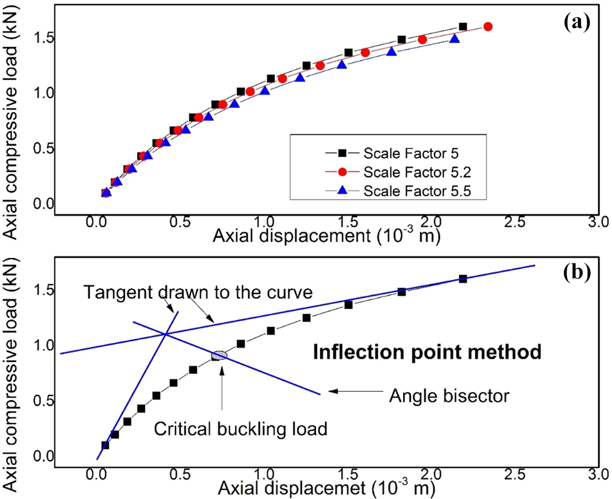
(a) Graph showing variations in nonlinear buckling analysis on taking into account scale factors (5, 5.2, 5.5) for 0.3 wt.% MWCNT-GE and (b) determination of critical load by inflection point method.

Experimental buckling test

The specimens are loaded as shown in Figure 2 and subjected to compressive load up to its fracture point. The load vs displacement graph is plotted for three specimens, 0 wt.% MWCNT-GE, 0.1 wt.% MWCNT-GE and 0.3 wt.% MWCNT-GE. The average of the test carried out on each specimen is plotted as shown in Figure 8. The buckling load was found out using the inflection point method (Figure 7)³¹ and its values are tabulated in Table 2. The stiffness in the composite column is captured using the slope of the tangent in the pre-buckling region. It is observed that stiffness increases with an increase in MWCNT, and is shown in Table 2.

Figure 8.

Average buckling curve.

It is found that by the addition of 0.1 wt.% MWCNT, the buckling load has increased by 14.81% and with 0.3 wt.% MWCNT the buckling load has increased by 27.4% in comparison to GE-Composite. Thus, the addition of MWCNT has improved the mechanical properties like stiffness, flexural modulus, and critical buckling load thereby increasing the buckling stability of the structure.

The presence of nanomaterials in very small proportions has enabled to distribute the load and reduce its effects. Due to the high aspect ratio of the MWCNT, the load gets distributed and hence acts as a reinforcement at the nano level. The fractured surfaces are as shown in Figure 9. It is seen that the composite is brittle even though it’s hard. After the elastic region the structure buckles and undergoes a very short plastic region for few millimeters and then ruptures. In Figure 9(b) shown, the structure still retains the fibers in it. The matrix fails but there are still links between the glass fibers that hold the structure together. This shows that the failure is initiated at the micro-levels of the epoxy matrix.

Figure 9.

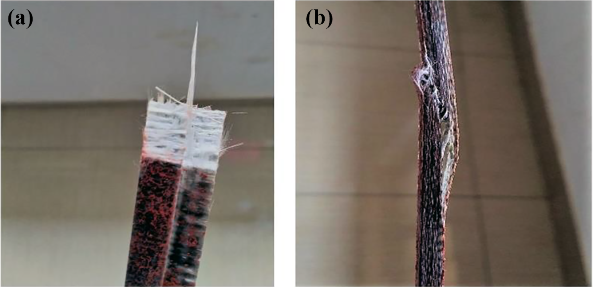
Fractured surface of the specimen: (a) front view after tearing and (b) side view after tearing.

Comparison study

The comparison study was done between the analytical, numerical, and experimental methods used to find the critical buckling load.

Scale factors of 5, 5.2, and 5.5 are used for the numerical simulation conducted to have a close comparison with experimental results and are plotted as shown in Figure 10. As the MWCNT concentration increases a deviation from numerical and experimental results is seen as the load sharing capacity between nanocomposites could not be accounted for in the numerical analysis. The buckling loads found using the inflection point method are shown in Table 2. The tabulated results obtained using the LBMI method showed that 0.1 wt.% MWCNT increases the buckling load by 19% and 0.3 wt.% MWCNT increases by 28%. The critical buckling loads obtained through different aforementioned methods are tabulated in Table 2.

Figure 10.

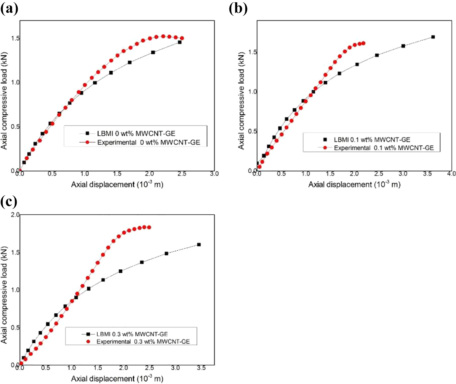
Numerical and experimental results comparison of specimens prepared: (a) scale factor 5 for 0 wt.% MWCNT-GE, (b) scale factor 5.2 for 0.1 wt.% MWCNT-GE and (c) scale factor 5.5 for 0.3 wt.% MWCNT-GE.

The analytical and eigenvalue buckling formulations over predicts the values of the critical buckling load. This can be attributed to the assumption of a structure without any imperfection. Since the values obtained are for the ideal case and the actual value of the buckling load could be 0–40% lower than the eigenvalue buckling. The trend is very evident from the experimental and nonlinear buckling analysis. The LBMI method that closely approximated the buckling value shows a similar trend to that of the experimental results. The errors are due to assumptions made (isotropic nature), and the end shortening effects that are not considered in the numerical scheme. The closeness of critical buckling values to the experimental proves that the numerical scheme LBMI approximates the solution correctly with some factor of safety.

Conclusion

The effect of different wt.% of MWCNT on the buckling behavior of MWCNT-GE nanocomposite is investigated. The XRD results revealed the presence of s-MWCNT embedded inside the composite specimen. The experimental investigations proved that with the increase in wt.% of MWCNT content, the critical buckling load is found to increase which could be attributed to the increase in flexural modulus with different wt.% of MWCNT. The LBMI method closely approximated the critical buckling load with that of the experimental value and the load vs displacement is comparable. It initiates the broader reach of nanocomposite technologies to be used in cases where compressive loads work. The presence of nanomaterials as fillers can improve the structural stability of different structures subjected to compressive loads.

Footnotes

Declaration of conflicting interests

The author(s) declared no potential conflicts of interest with respect to the research, authorship, and/or publication of this article.

Funding

The author(s) received no financial support for the research, authorship, and/or publication of this article.

ORCID iD

Nivish George

References

Chow

Tan

. Epoxy/multiwall carbon nanotube nanocomposites prepared by sonication and planetary mixing technique. J Reinf Plast Compos 2010; 29(15): 2331–2342.

Iijima

. Helical microtubules of graphitic carbon. Nature 1991; 354(6348): 56–58.

McNally

Pötschke

Halley

, et al. Polyethylene multiwalled carbon nanotube composites. Polymer 2005; 46(19): 8222–8232.

Thostenson

Ren

Chou

. Advances in the science and technology of carbon nanotubes and their composites: a review. Compos Sci Technol 2001; 61(13): 1899–1912.

Shonaike

Advani

. Advanced polymeric materials: structure property relationships. Boca Raton, FL: CRC Press, 2003.

Byrne

Gun’ko

. Recent advances in research on carbon nanotube–polymer composites. Adv Mater 2010; 22(15): 1672–1688.

Cho

Daniel

. Reinforcement of carbon/epoxy composites with multi-wall carbon nanotubes and dispersion enhancing block copolymers. Scripta Mater 2008; 58(7): 533–536.

Gojny

Wichmann

Fiedler

, et al. Influence of nano-modification on the mechanical and electrical properties of conventional fibre-reinforced composites. Compos A Appl Sci Manuf 2005; 36(11): 1525–1535.

Kim

Park

Okoli

, et al. Processing, characterization, and modeling of carbon nanotube-reinforced multiscale composites. Compos Sci Technol 2009; 69(3–4): 335–342.

10.

Thostenson

Chou

. Carbon nanotube networks: sensing of distributed strain and damage for life prediction and self healing. Adv Mater 2006; 18(21): 2837–2841.

11.

Wichmann

Sumfleth

Gojny

, et al. Glass-fibre-reinforced composites with enhanced mechanical and electrical properties—benefits and limitations of a nanoparticle modified matrix. Eng Frac Mech 2006; 73(16): 2346–2359.

12.

Garcia

Wardle

Hart

, et al. Fabrication and multifunctional properties of a hybrid laminate with aligned carbon nanotubes grown in situ. Compos Sci Technol 2008; 68(9): 2034–2041.

13.

Iwahori

Ishiwata

Sumizawa

, et al. Mechanical properties improvements in two-phase and three-phase composites using carbon nano-fiber dispersed resin. Compos A Appl Sci Manuf 2005; 36(10): 1430–1439.

14.

Seyhan

Tanoglu

Schulte

. Mode I and mode II fracture toughness of E-glass non-crimp fabric/carbon nanotube (CNT) modified polymer based composites. Eng Frac Mech 2008; 75(18): 5151–5162.

15.

Park

Lee

. Compression molding in polymer matrix composites. In: Advani

Hsiao

K-T

(eds) Manufacturing techniques for polymer matrix composites (PMCs). Sawston: Woodhead Publishing, 2012, pp. 47–94.

16.

Khang

Rogers

Lee

. Mechanical buckling: mechanics, metrology, and stretchable electronics. Adv Funct Mater 2009; 19(10): 1526–1536.

17.

Dasgupta

Haslach

. Mechanical design failure models for buckling. IEEE Trans Reliabil 1993; 42(1): 9–16.

18.

Rathore

Prusty

Kumar

, et al. Mechanical performance of CNT-filled glass fiber/epoxy composite in in-situ elevated temperature environments emphasizing the role of CNT content. Compos A Appl Sci Manuf 2016; 84: 364–376.

19.

Meyers

Chawla

. Mechanical behavior of materials. Cambridge: Cambridge University Press, 2008.

20.

Tam

Ruan

Gao

, et al. High-performance ballistic protection using polymer nanocomposites. In: Sparks

(ed) Advances in military textiles and personal equipment. Sawston: Woodhead Publishing, 2012, pp. 213–237.

21.

Sankal

Kaynak

. Using various techniques to characterize oxidative functionalized and aminosilanized carbon nanotubes for polyamide matrix. J Reinf Plast Compos 2013; 32(2): 75–86.

22.

Holzwarth

Gibson

. The Scherrer equation versus the ‘Debye-Scherrer equation’. Nat Nanotechnol 2011; 6(9): 534.

23.

Timoshenko

Gere

. Theory of elastic stability. North Chelmsford: Courier Corporation, 2009.

24.

Khot

Venkayya

. Effect of fiber orientation on initial postbuckling behavior and imperfection sensitivity of composite cylindrical shells. Wright-Patterson AFB, OH: Air Force Flight Dynamics Lab, 1970.

25.

Hühne

Rolfes

Breitbach

, et al. Robust design of composite cylindrical shells under axial compression—simulation and validation. Thin-Walled Struct 2008; 46(7–9): 947–962.

26.

Taheri-Behrooz

Omidi

Shokrieh

. Experimental and numerical investigation of buckling behavior of composite cylinders with cutout. Thin-Walled Struct 2017; 116: 136–144.

27.

Jia-Jia

Xin

Qiu-Jie

, et al. The preparation of nano-sulfur/MWCNTs and its electrochemical performance. Electrochim Acta 2010; 55(27): 8062–8066.

28.

Liu

Zhang

Wang

, et al. Effects of cure cycles on void content and mechanical properties of composite laminates. Compos Struct 2006; 73(3): 303–309.

29.

Chisholm

Mahfuz

Rangari

, et al. Fabrication and mechanical characterization of carbon/SiC-epoxy nanocomposites. Compos Struct 2005; 67(1): 115–124.

30.

Prashantha

Soulestin

Lacrampe

, et al. Masterbatch-based multi-walled carbon nanotube filled polypropylene nanocomposites: assessment of rheological and mechanical properties. Compos Sci Technol 2009; 69(11–12): 1756–1763.

31.

Czapski

Kubiak

. Selected problems of determining critical loads in structures with stable post-critical behaviour. Mech Mech Eng 2016; 20(2): 79–95.

Mechanical buckling of nanocomposites: Experimental and numerical investigations

Abstract

Keywords

Introduction

Experimental details

Fabrication of nanocomposites

Materials

Fabrication of mold

Fabrication of (glass epoxy) GE composite

Fabrication of MWCNT-GE nanocomposite

Material characterization

Buckling analysis

Analytical analysis

Numerical analysis

Linear buckling analysis

Nonlinear buckling analysis

Experimental analysis

Results and discussion

X-ray diffraction

Density test

Flexural test

Buckling test

Analytical solution

Numerical analysis

Linear buckling analysis

Nonlinear buckling analysis

Experimental buckling test

Comparison study

Conclusion

Footnotes

Declaration of conflicting interests

Funding

ORCID iD

References