Chemical and appearance changes of wood due to artificial weathering – Dose–response model

Abstract

The aim of this study was to assess a model for the surface degradation kinetics of natural wood exposed to artificial weathering. The photochemical and physical processes of weathering result in simultaneous changes of both the wood matrix composition (i.e. lignin content, cellulose crystallinity index, cellulose polymerization degree) and wood’s appearance (i.e. colour, gloss, roughness). European larch, a popular cladding material, was used for experimental samples. Weathering was conducted in a QUV artificial weathering machine for 672 h according to the EN927-6 standard. The response of wood was assessed using multi-sensor measurements. Results revealed that changes in colour are evident already after 28 h of artificial weathering, with an increase in a* and b*, and a decrease in L*. That initial trend was reversed afterward, with the colour changing to grey. Due to the particular shape of the curves representing colour coordinates, it is difficult to use CIE L*a*b* parameters to model the weathering dose. However, the degradation curve established for selected near infrared bands was useful to build a dose–response model of wood surface degradation. In all cases, a clear trend of change in absorbance values that progressed along with the weathering dose was observed. These curves, unlike the CIE L*a*b* values, are monotonic, meaning that dose value corresponded with only one value of absorbance. Principal component analysis of the near infrared spectra allowed clustering of the spectra by different dose classes, with the main differentiation in the reference class and in the final class (maximum dose). It was found that the discrimination between spectra at diverse cumulative weathering doses was more evident for earlywood than for latewood. This confirms the hypothesis that degradation kinetics differ depending on the anatomical configuration of wood. This research is a first step for establishing dose–response model for natural weathering, where precise quantification of weathering parameters is more challenging.

Introduction

Wood weathering is the process of surface alteration caused by exposure of wood to abiotic degradation factors. This process results in changes to several wood features such as colour, gloss and surface topography. ¹ The structural and mechanical properties of wood remain intact initially during this process, which affects a few microns of surface depth, at the interface between wood and atmosphere. ² Nonetheless, weathering can create a more compliant situation for biotic colonization, thus beginning severe enzymatic decomposition of the wood. For instance, natural weathering was shown to significantly decrease hydrophobicity of wood, resulting in increased short-term water uptake of aged wood. ³ The increase in moisture can then promote favourable conditions for wood-decaying fungi. Moreover, ultraviolet (UV) radiation can cause a decrease in the softening temperature of lignin, measured through the dimensional variation of a material under increasing temperature. ⁴ In fact, one of the major effects of weathering is the degradation of lignin by UV light, ⁵ since lignin is the most sensitive compound in wood to UV photodegradation.^6,7 Degradation of lignin by UV radiation has been shown to affect sorption–desorption of water vapour, reducing the moisture affinity of wood until leaching takes place. ⁸ Weathered wood veneers possess a noticeable higher content of ethanol- and water-soluble compounds compared to non-weathered wood. ⁵ Moreover water-soluble sugars (e.g. mannose, xylose and glucose) found in water extracted from weathered wood are by-products of the degradation of hemicellulose and cellulose. ⁵ Alternate wetting–drying and/or freezing–thawing cycles can cause delamination and crack formation that facilitate the creation of micro-habitats favourable to wood-decaying fungi and reduce the aesthetical and structural functions of wood. Weathering experiments show that chemical modifications of the wood matrix occur already after short exposure to UV light and water. ¹ These chemical modifications are revealed through colour changes in weathered wood. The CIE L*a*b* colour coordinates system is widely used to represent colours in three-dimensional space. The visible, short exposure time effect of lignin degradation is an increase in the b* value, with a yellowing of the wood ⁹ that is caused by the formation of chromophoric groups of secondary origin. ⁶ When the chromophoric groups leach from the wood, the wood colour changes further, eventually converting to grey shades.

Since ancient times protective treatments have been used to improve the performance of woody materials for outdoor use. Protection of external wood is obtained through several systems: coating, chemical modification (i.e. substitution of –OH groups by acetyl groups), additives that trap radicals, thermal and/or photochemical pre-weathering and use of UV absorbers. ¹⁰ New wood modification processes that are not harmful to the environment (i.e. without biocides) emerged recent years, driven mainly by a general increase in environmental awareness. ¹¹ In this context, the use of natural, untreated wood may have several advantages (i.e. economic, environmental). ¹² For example, in Germany, multiple re-use cycles of waste wood are only possible when the dismantled wood is classified as non-treated, while for treated wood fewer options are permitted, due to the presence of treatment chemicals and/or other substances. ¹³ Other European countries (i.e. UK, Italy, Finland) developed similar systems of waste wood classification to impose control over the so-called reverse supply chain of wood (i.e. the supply of waste wood for re-use). ¹³

Nonetheless, a major restraint for choosing natural wood for external use is the lack of confidence that architects, designers and customers have towards this material, mostly due to aesthetic preferences. The speed and pattern of the colour change are difficult to predict and are rarely taken into consideration at the early phases of building design. Natural weathering changes the wooden building appearance; however, in some case this change might be desired especially in the local context, as presented in Figure 1, where a rustic wooden chalet constructed with unprotected larch is well integrated with the mountain landscape.

Figure 1.

Appearance change of a traditional wooden house in the North-eastern Italian Alps in 2003 (a) and in 2017 (b). Source: (a) www.regolespinalemanez.it (accessed 24 July 2018) and (b) Grossi Paolo.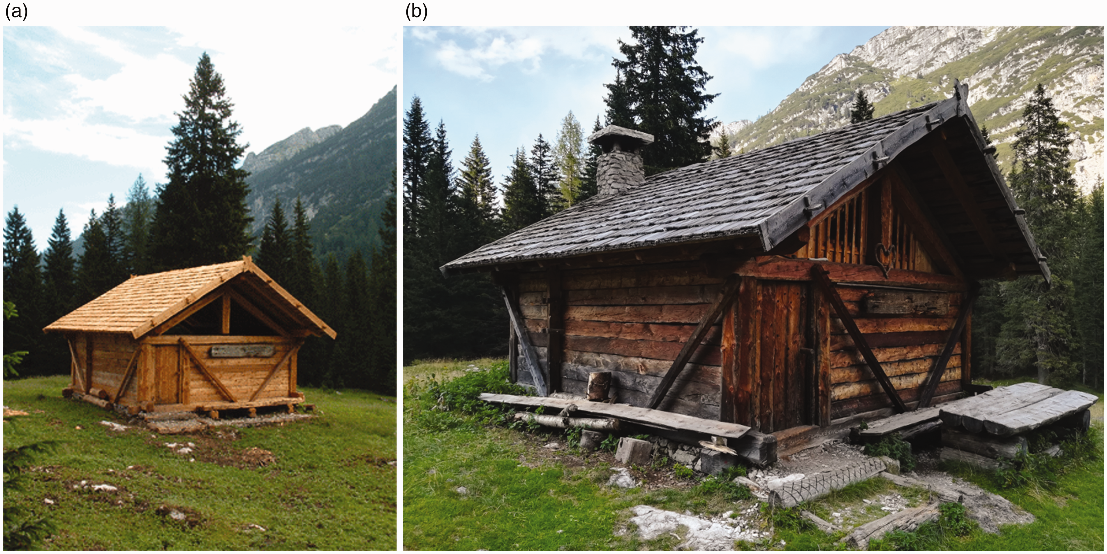

Experimental data from natural or artificial weathering tests can be used to model the colour changes of wood. ¹⁴ These models can then be used to simulate the appearance of weathered wooden facades over time. ¹⁵ However, many factors are involved in the aesthetic changes of a building, such as wood type, design of the building and climate, are interconnected. Therefore, constructing a model that considers all factors and their interactions is particularly challenging. Moreover, the external appearance of wood results from differential weathering of heterogeneous zones within the tree rings (i.e. earlywood and latewood).^16,17 Understanding of the weathering kinetics of earlywood and latewood separately is important for realistic simulations of wood patterns, thus improving the quality of the architectural rendering. For this purpose, several spectroscopic techniques can be used, such as Fourier-transform near infrared spectroscopy and hyperspectral imaging.^18,19 The spectroscopic data can be merged and analysed by chemometric techniques (e.g. principal component analysis (PCA))^17,20 that have been proven to be a valid tool to build predictive models of wood weathering.

The goal of this work was to develop a dose–response model for predicting major aesthetic surface properties (colour, gloss) as well as physical–chemical changes to the functional groups of wood polymers. Artificial weathering under controlled conditions allows the exact quantification of weathering doses to which samples are subjected. Consequently, changes in the appearance of wood and the chemical modifications that caused these changes were measured with a multi-sensor approach.

Materials and methods

Sample preparation and artificial weathering

Larch wood was selected for experimental specimens due to its frequent use as an untreated cladding material. Samples were obtained from a single stem of European larch (Larix decidua Mill.), which was cut in 52 wooden blocks with dimensions of 80 mm × 150 mm × 20 mm (tangential × longitudinal × radial direction, respectively). The standardized procedure for artificial weathering testing suggests exposure of the radial section wood surfaces with inclination of the growth rings from 0 to 45°. ²¹ However, a random mixture of radial and tangential samples was tested in this experiment, in order to mimic with the real variability occurring on industrial claddings. Five wood samples were not weathered but used as a reference. The remaining 47 samples were exposed to artificial weathering with UV radiation and water spraying cycles in a QUV accelerated weathering tester (Q-lab, Westlake, USA), with a varying number of weathering cycles per sample. Each full weathering cycle included 2.5 h of UV light radiation (UVA-340 lamp simulating solar radiation from 365 to 295 nm, with a peak emission at 340 nm) and 0.5 h of water spray. The changes in the irradiation intensity and the ambient temperature over time recorded during the three initial cycles of the test are presented in Figure 2. In this study, each completed cycle is defined as a single weather dose received by the wood. The configuration of the QUV sample compartment allowed a maximum of 24 samples to be exposed simultaneously. All of these were filled with larch wood samples and the testing procedure was initiated (after pre-treatment samples were weathered with different numbers of doses). It has to be mentioned that the standard procedure for artificial weathering according to EN 927-6 (Cycle 1 on QUV accelerated weathering tester) includes pre-treatment and post-treatment phases where samples are exposed to 24 h of water condensation at 45℃ without any UV irradiation. 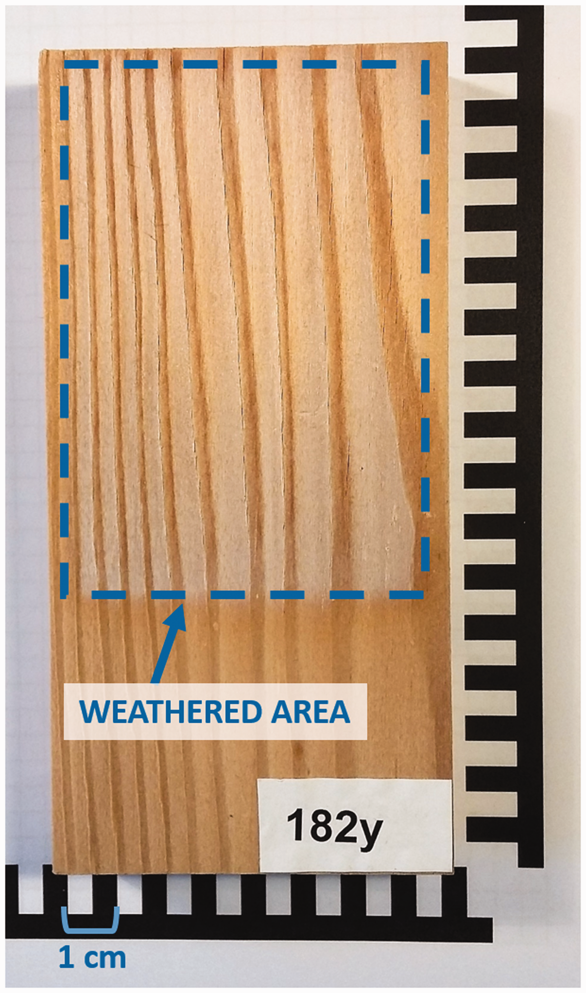²¹ A single weathered sample was removed regularly from the QUV machine and was replaced by a fresh one. For that reason, the number of doses received by each sample varied and ranged from 7 to 208. The individual weathering history was recorded as a sample code, where a number corresponded to the total number of doses absorbed. The additional character (symbol ‘y’) distinguished sample exposed to the 24 h pre-treatment from those post-treated (symbol ‘n’). An example of a wooden sample after 182 doses (artificial weathering cycles) including pre-treatment is presented in Figure 3. The specific configuration of sample holder allows weathering of only part of the sample highlighted in dashed blue line. All samples, including the un-weathered references were stored at a constant temperature of 20℃ and relative humidity of 65% in a dark room in order to ensure uniform conditioning and to prevent any further degradation.

Figure 2.

UV irradiance and air temperature changes over time during the three initial phases of the artificial weathering test performed in the QUV machine.

Figure 3.

Sample 182y after artificial weathering. The weathered area is highlighted in dashed blue line.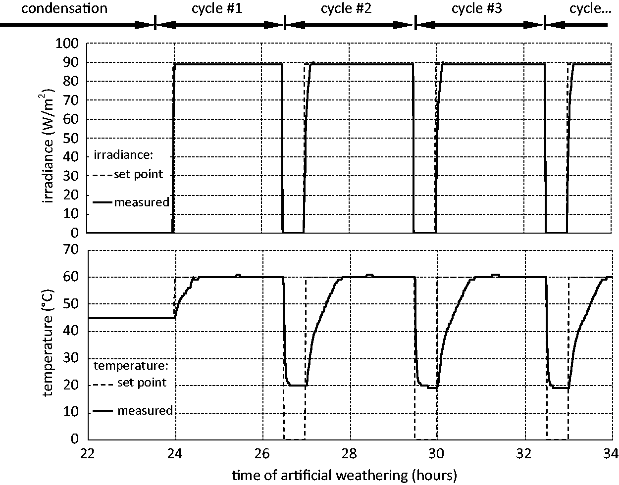

Colour measurement

Changes in colour were assessed by a spectrometer following the CIE Lab system where colour is expressed with three parameters: L* (lightness), a* (red-green tone) and b* (yellow-blue tone). CIE L*a*b* colours were measured using MicroFlash 200D spectrophotometer (DataColor Int, Lawrenceville, USA). The selected illuminant was D65 and viewer angle was 10°. All specimens were measured on six different spots over the weathered surface, with three measurements in earlywood and three in latewood. A dedicated mask was used to position the light beam precisely, pointing at earlywood and latewood separately. The total colour change ΔE was calculated from the L*, a*, b* coordinates measured on the weathered sample (d) in comparison to the reference samples (0) according to the following formula (equation (1))

$$\Delta E=\sqrt{[(L_d^{*}-L_o^{*}{)}^2+(a_d^{*}-a_o^{*}{)}^2+(b_d^{*}-b_0^{*}{)}^2]}$$

(1)

Gloss measurement

The mode of light reflection from the surfaces was measured using a REFO 60 (Dr. Lange, Düsseldorf, Germany) gloss meter with incidence angle of 60°. Ten measurements were taken in total on each specimen, following two directions: along and across the fibre direction. It was not possible to measure earlywood and latewood separately due to the large size of the gloss meter’s measurement spot.

Near infrared (NIR) spectroscopy

NIR spectra were collected with a Vector N-22 Fourier-transform NIR spectrometer produced by Bruker Optics GmbH (Ettlingen, Germany). The system was equipped with a fibre optic probe and the measurement range was between 12,000 and 4000 cm⁻¹ (833 and 2500 nm). The fibre optic measurement spot was 10 mm², allowing separate measurement of early and late wood zones in most samples (depending on their exposed surface). The spectral wavenumber interval was 3.85 cm⁻¹ with zero filling equal to 2. The spectral resolution was 8 cm⁻¹ and 32 internal scans were averaged at each spectrum. The background was measured every hour on Spectralon® resin. The bands were assigned according to Schwanninger et al. ²² (Table 1).

Table 1.

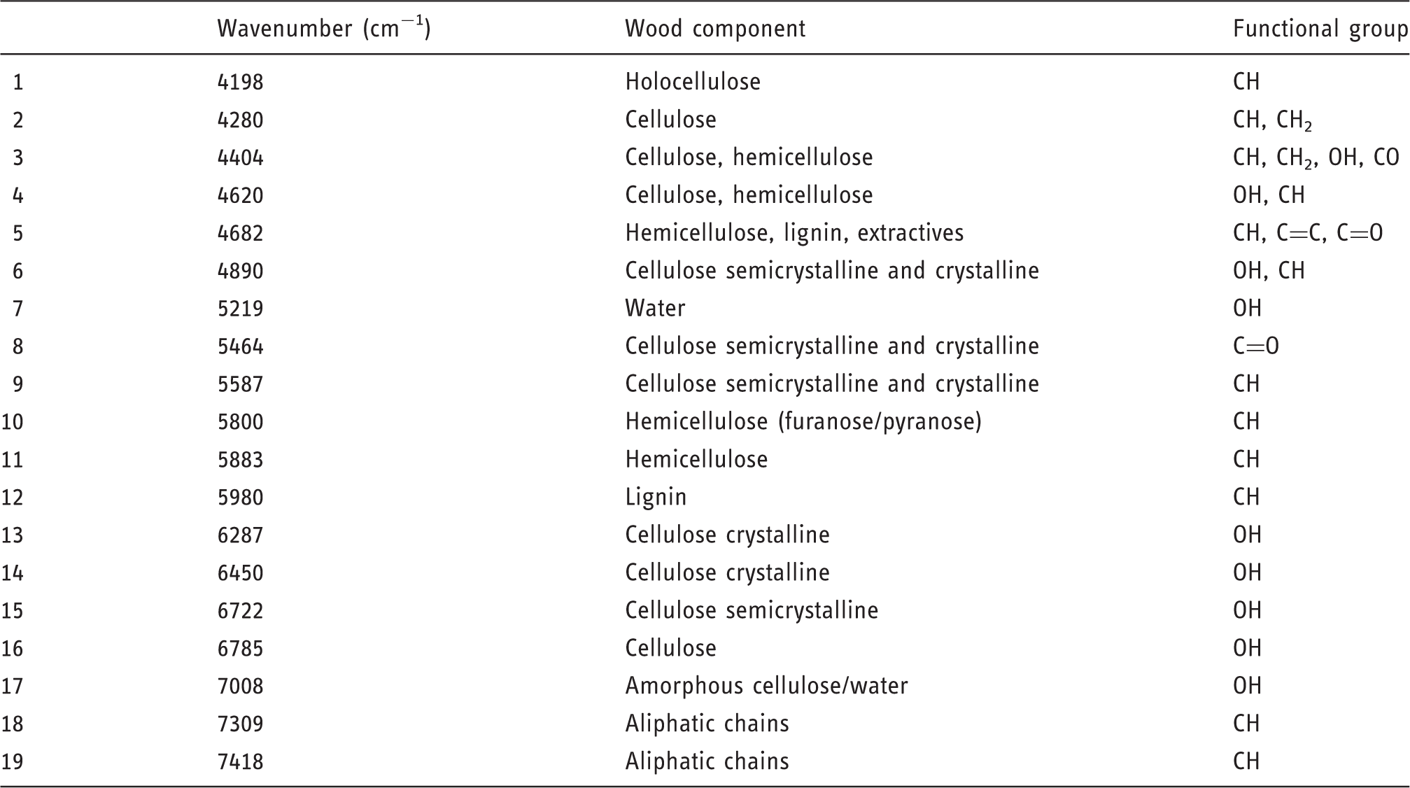
NIR band assignment for wood according to Schwanninger et al. ²²

	Wavenumber (cm−1)	Wood component	Functional group
1	4198	Holocellulose	CH
2	4280	Cellulose	CH, CH2
3	4404	Cellulose, hemicellulose	CH, CH2, OH, CO
4	4620	Cellulose, hemicellulose	OH, CH
5	4682	Hemicellulose, lignin, extractives	CH, C=C, C=O
6	4890	Cellulose semicrystalline and crystalline	OH, CH
7	5219	Water	OH
8	5464	Cellulose semicrystalline and crystalline	C=O
9	5587	Cellulose semicrystalline and crystalline	CH
10	5800	Hemicellulose (furanose/pyranose)	CH
11	5883	Hemicellulose	CH
12	5980	Lignin	CH
13	6287	Cellulose crystalline	OH
14	6450	Cellulose crystalline	OH
15	6722	Cellulose semicrystalline	OH
16	6785	Cellulose	OH
17	7008	Amorphous cellulose/water	OH
18	7309	Aliphatic chains	CH
19	7418	Aliphatic chains	CH

Statistical and spectral analysis

Statistical analysis has been carried out on the collected data. All samples were sorted into classes prior to statistical analysis. This approach was adopted in order to identify statistically significant differences between groups and not singular samples having received various amount of dose. An arbitrary factor of 50 doses was selected to be the threshold separating classes. In this way, six classes were created: Ref.: non-treated or 0 doses, class A: 1–50 doses, class B: 51–100 doses, class C: 101–150 doses, class D: 151–200 doses and class E: 201–250 doses. Statistical comparisons between pairs of classes were tested using the Wilcoxon Rank Sum test (non-parametric t-test). Statistical differences among classes for the measured variables were tested using the Mann–Whitney test (non-parametric ANOVA), followed by the Bonferroni post hoc test. R software, version 3.4.3 (https://www.r-project.org/) was used for all statistical analysis.

The OPUS 7.0 (Bruker Optics GmbH, Ettlingen, Germany), PLS_Toolbox 8.0 (Eigenvector Research, Manson, USA) and LabView 13 (National Instruments, Austin, USA) software packages were used for spectral pre-processing and data mining. The raw spectra were pre-processed with the extended multiplicative scatter correction and second derivative (Savitzky-Golay, 21 smoothing points).

Results and discussion

Samples appearance – CIE L^*a^*b^* colours

Wood samples divided by dose class are presented in Figure 4. The changes in colour, which are visible by eye, are evident in class A, where samples appear darker and redder, as well as in classes B–E, where the red tones gradually fade. This was well represented in the CIE L*a*b* coordinates.

Figure 4.

Appearance of the reference samples and 47 samples of larch wood after artificial weathering.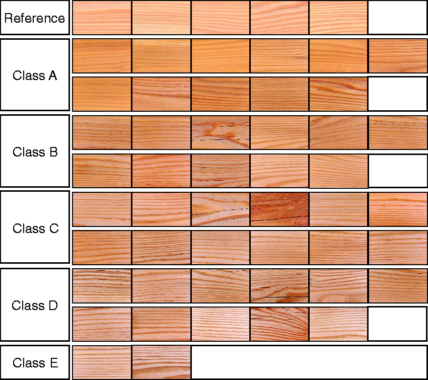

The differences between the L*, a* and b* values of earlywood and latewood are statistically significant (confidence interval 95%) or highly significant (confidence interval 99%), except in the case of reference samples CIE a* and b*; class A CIE L*, a* and b*; and class B CIE b* (Table 2). This indicates that earlywood and latewood of larch samples differ mostly for the lightness, and after the first doses of weathering, they reached similar colours in class A. With increasing weathering dose, the colours of earlywood and latewood diverge in all CIE parameters.

Table 2.

Significance level (p-value) of differences between earlywood and latewood tested with the Mann–Whitney Rank Sum test, first for all the samples taken together and then within each class of dose.

	p-values
	CIE L	CIE a	CIE b
All samples	0.039*	0.007*	0.001**
Reference	0.032*	0.209	0.222
Class A	0.365	0.131	0.178
Class B	0.030*	0.003**	0.065
Class C	0.006*	0.010*	0.004**
Class D	0.013*	0.002**	0.001**
Class E	–	–	–

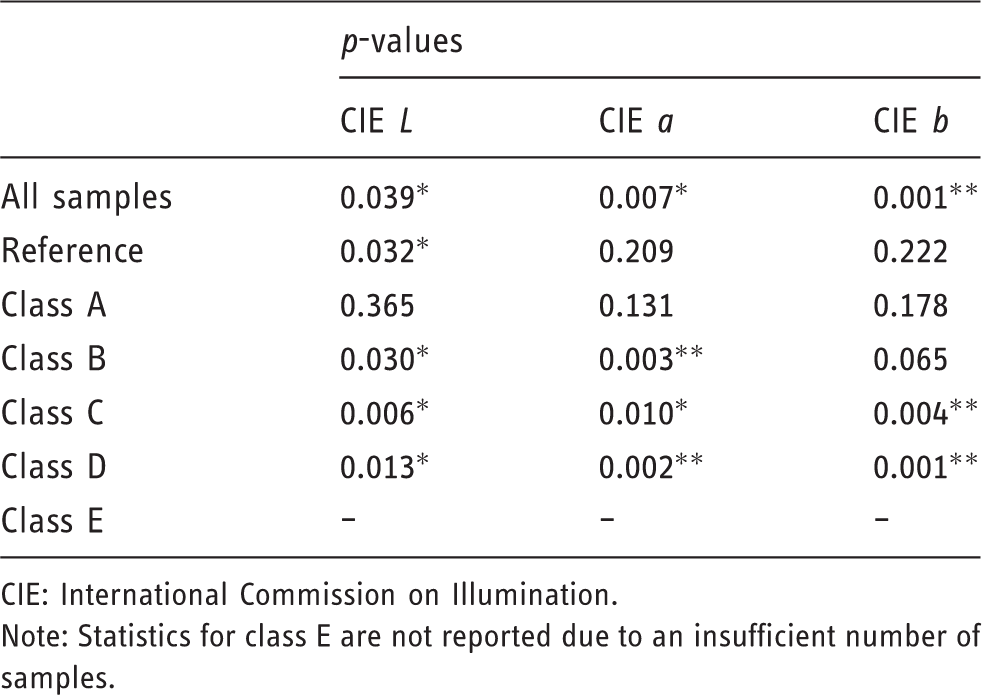
CIE: International Commission on Illumination.

Note: Statistics for class E are not reported due to an insufficient number of samples.

The changes in colour are already evident after 28 h of artificial weathering. The first class of weathered samples (A) has, on average, significantly lower L* values, but higher a* and b* values, when compared to the reference samples. With increasing doses, the L* values increase slightly, almost reaching the reference lightness values. The a* and b* value decreased after the initial rise, reaching values far below the reference at the final stage of exposure (Figure 5).

Figure 5.

Colour coordinates CIE L*, a* and b*, for earlywood and latewood, grouped by classes of dose. Different letters on the boxes indicate statistically significant differences according to Bonferroni post hoc test. Note: The black thick line indicates mean value, the bar corresponds to the data range (minimum and maximum), the box corresponds to the first and third quantiles, with the middle line corresponding to the median. CIE: International Commission on Illumination.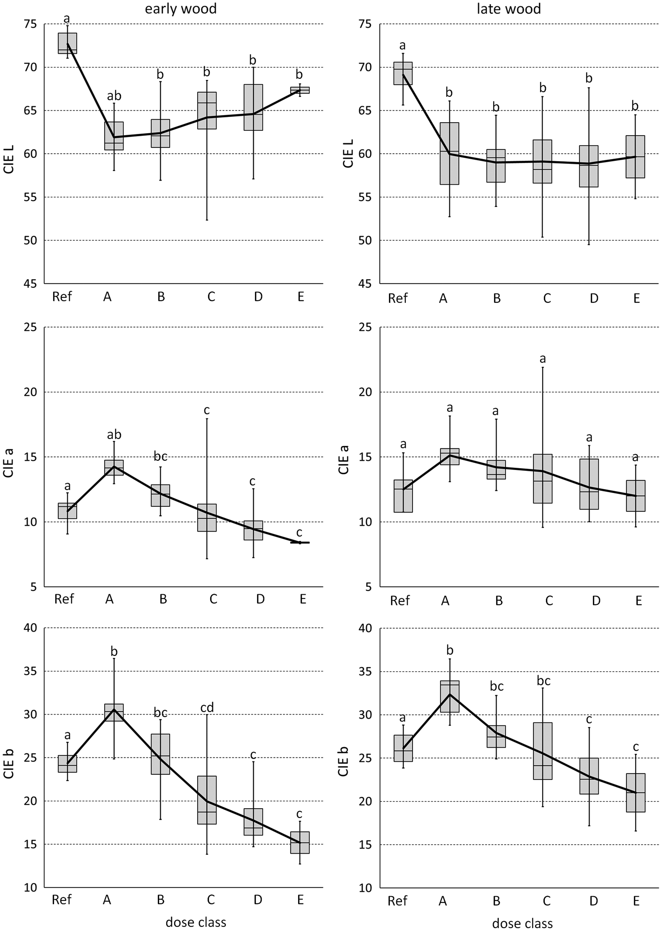

Due to the particular shape of the curves representing colour coordinates (e.g. decrease followed by slight increase for the L* value for earlywood, or initial rise for a* and b* values for both early and late wood, followed by a decrease) it is difficult to directly use these parameters to model the weathering dose. Likewise, it is evident that the wood might have similar colour values after receiving different weathering doses (e.g. reference samples and samples in class E have similar CIE a* values of latewood colour). The colour parameters in these cases seem to be inadequate for establishing a numerical dose–response model.

On average, the L*a*b* values of the reference samples are in the range of those present in the literature for European larch wood.^23,24 The pattern of initial increase of a* and b*, followed by their decrease, is also reported by other authors.^6,9,25 This was explained with in situ reactions, involving lignin degradation and the photooxidation of –CH₂– and –CH(OH)– groups, with the formation of secondary chromophoric structures (quinones). The mechanism of the silver or grey patina generation on the wood surface exposed to weathering is attributed to the formation of secondary chromophoric structures ⁶ followed by the birefringence of cellulose due to the UV degradation of amorphous cellulose and the selective preservation of crystalline cellulose.^2,6 In the final stage, the chromophoric structures are leached from the wood by rain water. ²⁶

Total colour change and normalized total colour change

The total colour change in each class is presented in Figure 6, where ΔE has been normalized by dividing it by the specific dose for each sample. At the initial stage (class A) the total colour difference was higher and diminished as weathering progressed. Samples assigned to classes C, D and E have similar values of ΔE. However, as weathering progressed and with the consequent increase in the received doses, the variation of ΔE diminished within the classes. This means that the natural variability in colour clearly visible in the samples at the beginning of the experiment (high value scatter in class A) is reduced and samples possess a more uniform colour at the final stage of the weathering experiment (low data range in class E).

Figure 6.

The total colour change normalized for the dose value as represented for earlywood (light grey boxes) and for latewood (white boxes) in classes A–E. Note: The bar corresponds to the data range (minimum and maximum), the box corresponds to the first and third quantiles, with the middle line corresponding to the median.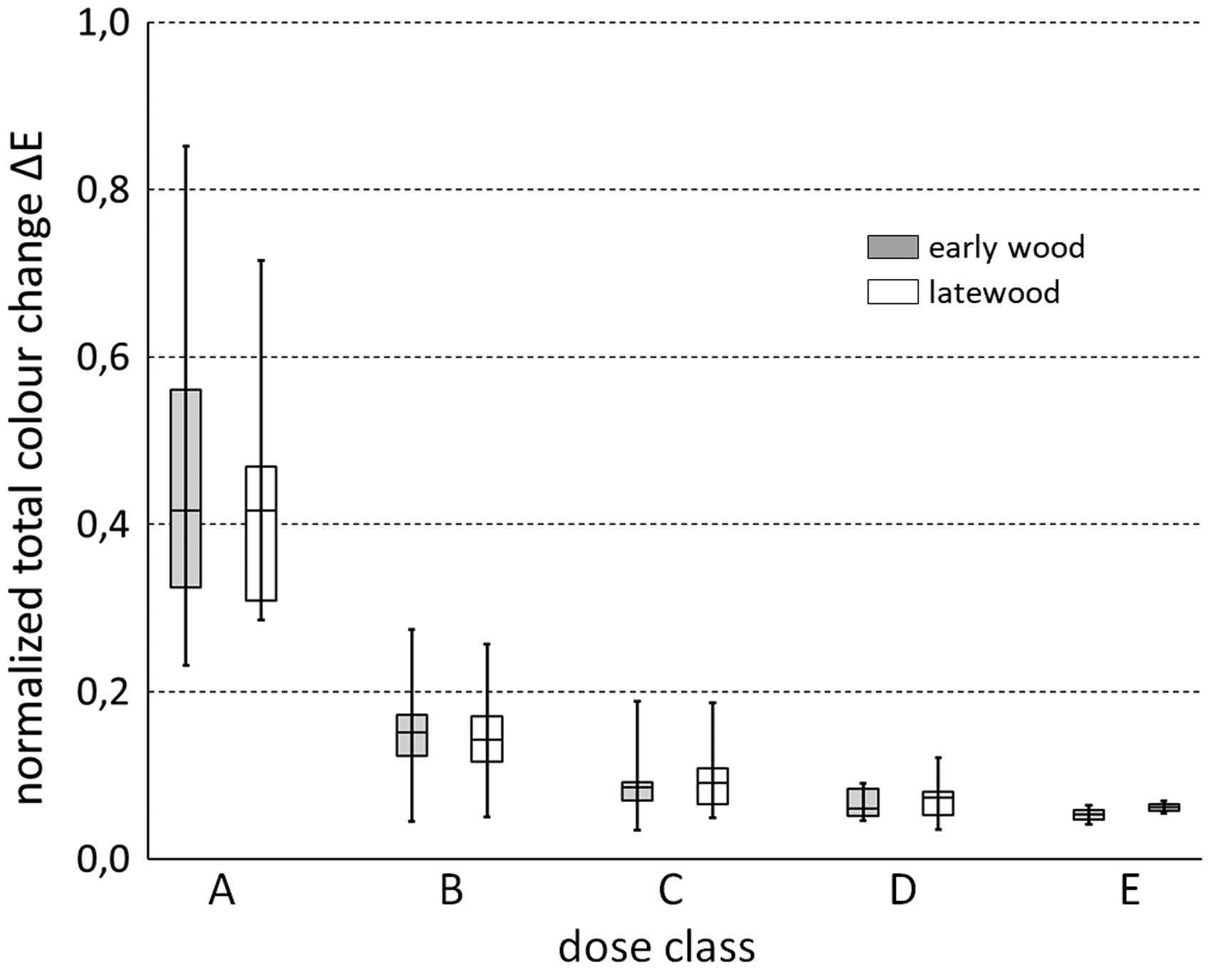

The non-normalized values of ΔE are presented separately for earlywood and latewood and for pre- and post-treated samples (Figure 7). An effect of the pre- and post-treatment is evident for earlywood in the first dose class (A), where pre-treated samples show a greater total colour change. A statistically significant difference in pre- and post-treated samples is also found in latewood, but in this case in the last final dose class (E).

Figure 7.

Effect of the pre-treatment and post-treatment on earlywood and latewood colour change due to weathering. Note: The bar corresponds to the data range (minimum and maximum), the box corresponds to the first and third quantiles, with the middle line corresponding to the median. (a) Earlywood and (b) latewood.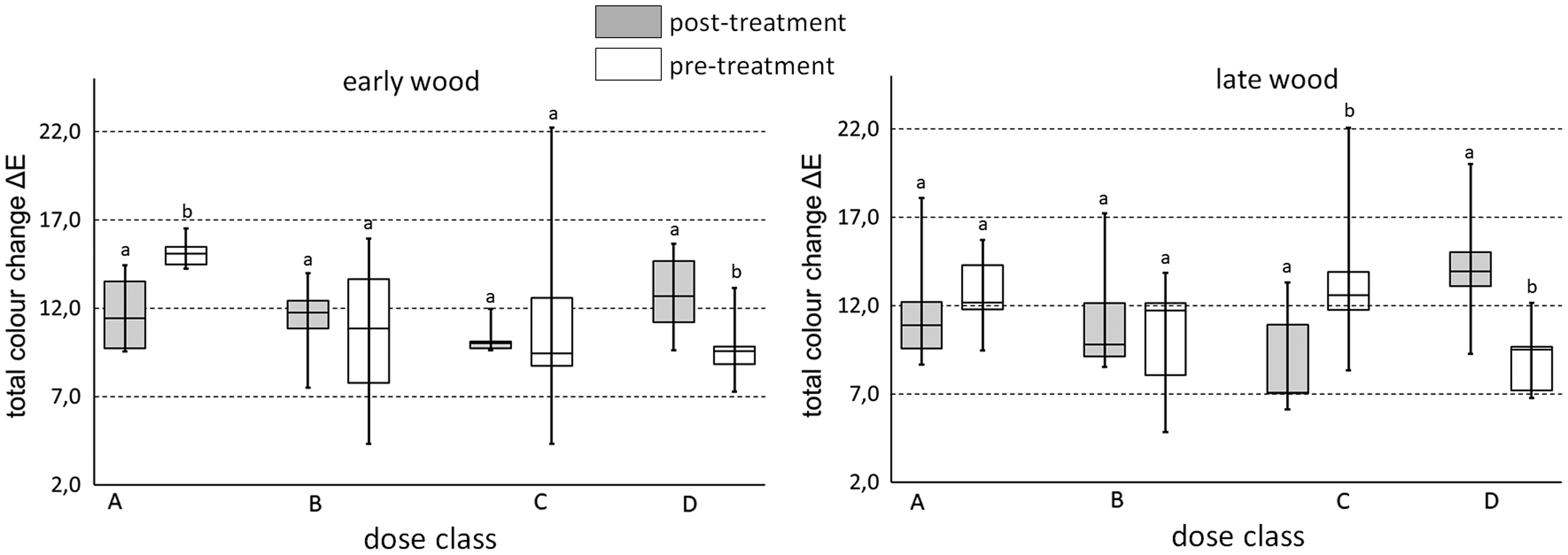

Gloss evaluation

The gloss increased with weathering duration, both along and across the fibres, and it was highest along than across the fibres (Figure 8). There are few studies that report the gloss of natural wood without coatings. Some authors observed a decrease in gloss after one year of natural weathering, ²⁰ while others found an initial increase during the first six months, which was then followed by a decrease. ²⁴ Gloss changes result from the abrasion of wood surfaces and the accompanying erosion process. Initial increases in glossiness might be explained by the regular removal of degradation products. ¹ Often gloss reduction is reported in the later stages of weathering and is caused by surface checking and raised grain. Observation of gloss changes is particularly useful while assessing and evaluation of coating systems. According to Pánek et al., ²⁷ gloss change is more sensitive to coating degradation than to total colour difference.

Figure 8.

Surface gloss measured along the fibres (light grey) and across the fibres (white). Note: Different letters on the boxes indicate statistically significant differences according to Bonferroni post hoc test with gloss along the fibres (letters without brackets) and across the fibres (letters in brackets). The bar corresponds to the data range (minimum and maximum), the box corresponds to the first and third quantiles, with the middle line corresponding to the median.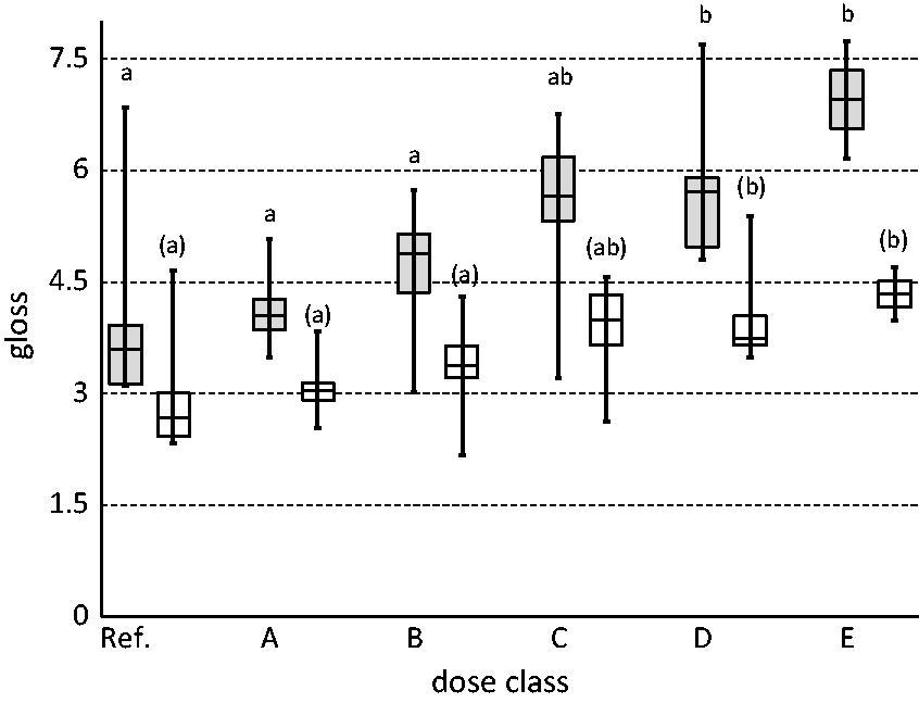

NIR spectroscopy

The second derivative spectra of earlywood at different stages of artificial weathering (doses 0, 105 and 208) are presented in Figure 9. Absorbance of –CH functional groups of carbohydrates (both cellulose and hemicellulose) (band 3), hemicellulose (band 10) and lignin (band 12) was different compared to the references (i.e. un-weathered samples). The absorbance in the second derivative is lower, which means that the quantity of the functional groups diminished. The most pronounced reduction of intensity is evident for band 12 and is related to the degradation of lignin caused by UV radiation. It is evident that the spectra of samples receiving 105 and 208 doses have similar absorbance, which means that the degradation occurs relatively fast and seems to have been slower in the second part of the artificial weathering test. A similar trend was observed for band 5 (hemicelluloses, lignin and extractives). Samples receiving 105 and 208 doses possess very similar values of absorbance. Intense initial leaching of extractives is observed in species possessing high extractives content, such as investigated larch. ²⁸ Changes in bands related to hydroxyl groups assigned to water and amorphous cellulose (band 7 and 17, respectively) were noticeable. This can be interpreted as a loss of –OH groups followed by wood dehydration stimulated by UV irradiation. However, very little change was observed in bands 13 and 14 that are assigned to crystalline regions of cellulose and bands 6, 8 and 9 corresponding to semicrystalline and crystalline cellulose. This confirms that those regions are more resistant against weathering. ¹⁸ Similar results were observed for the latewood, however with slightly different kinetics. –CH groups of hemicelluloses seem to be unaffected by weathering at the initial stage of the test (the second derivative of the absorbance for band 10 was almost identical to the reference and 105 dose values). However, –CH band 12 at 5986 cm⁻¹ (assigned to lignin) of 105 and 208 doses was similar, which means that degradation occurred at the first stage of weathering and was more constant in the second stage of the test.

Figure 9.

Second derivative of the absorbance for reference samples (dashed line), samples treated with 105 doses (light grey line) and 208 doses (black line) as measured on the early wood zone.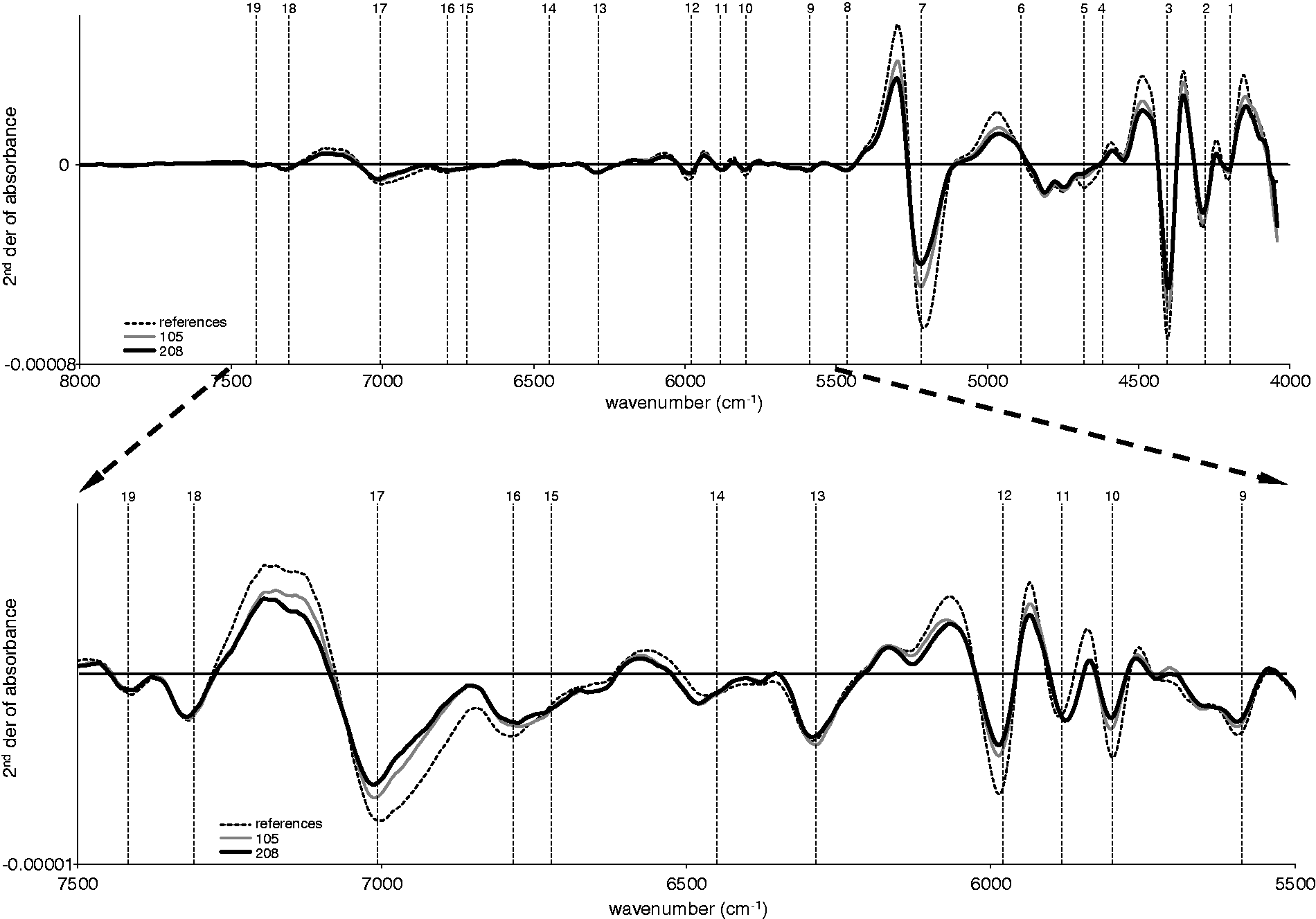

Values of the second derivative NIR spectra corresponding to selected bands with evident changes in absorbance (3: holocellulose, 5: hemicellulose, lignin, extractives, 10: hemicellulose and 12: lignin) are presented in Figure 10. In all cases, a clear monotonic trend in the absorbance value associated with increasing of weathering dose is observed. NIR spectroscopy data are therefore suitable for constructing dose–response models of the artificial weathering of wood.

Figure 10.

Changes in the second derivative of the NIR absorbance spectra for the –CH bands of different wood polymers with the progress of weathering; carbohydrates (4404 cm⁻¹), hemicellulose, lignin, extractives (4682 cm⁻¹), hemicellulose (5801 cm⁻¹) and lignin (5986 cm⁻¹). Note: The spectra of the samples that were not pre-treated are marked in black, while those that were pre-conditioned before the test are white.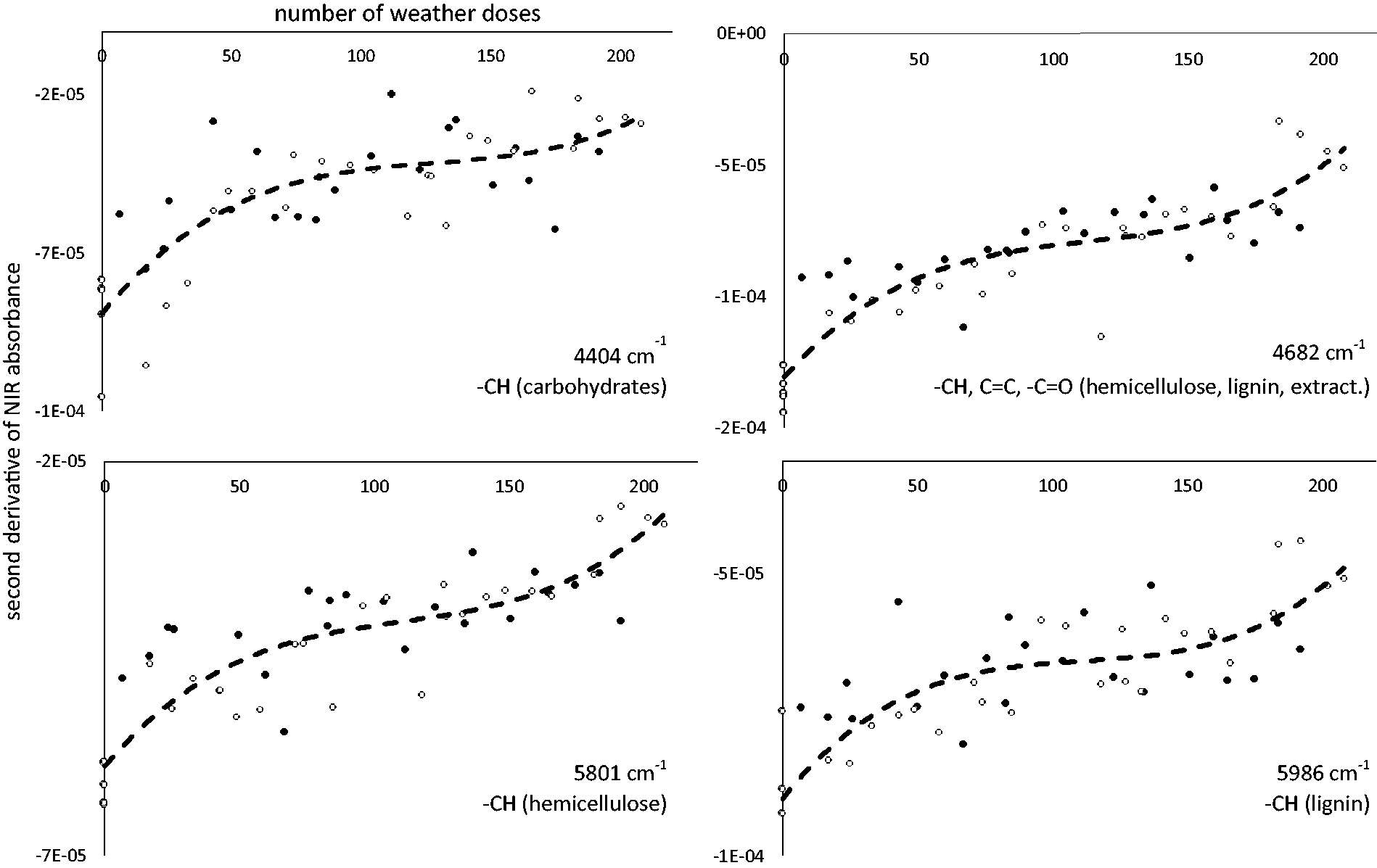

NIR spectroscopy and PCA

The PCA highlighted differences among samples exposed to different doses (Figure 11). However, as expected, not all a priori established classes of weathering were separated even though samples from overlapping classes followed a path as indicated by the arrow on the graph. The reference samples, for instance, were clearly separated from all treated samples, while most of the treated samples were clustered together in one large group, where a transition from class A to class D was not clearly evidenced. Nevertheless, samples treated with a higher number of cycles were grouped together in a separate cluster. The classification system used for the purpose of this research was arbitrary groups of 50 consecutive, increasing cycles of weathering per class. Even if it proved to be highly useful to highlight differences in colour and in chemical composition, it was not an optimal solution for discrimination of NIR spectra.

Figure 11.

PCA scores for NIR spectra of artificially weathered earlywood.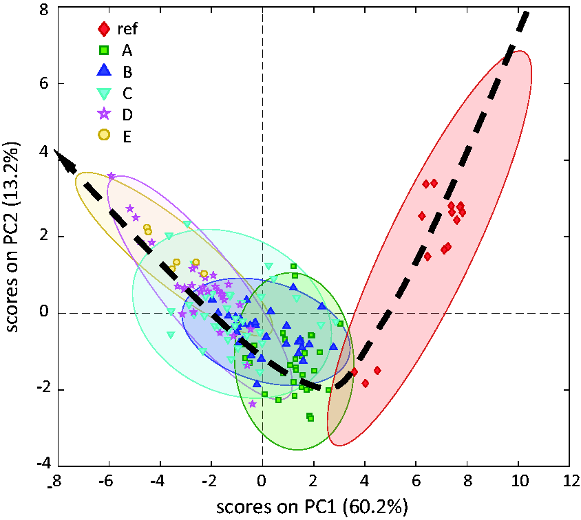

The spectral differences were relatively small (due to the limited time of the artificial weathering exposure) but followed a monotonic pattern of change that was slightly different for earlywood and latewood. The change of first principal component value in a function of the weathering intensity (number of doses) determined by independent PCA models is presented in Figure 12. The initial drop of PC1 value was highest in the case of earlywood, where the following decline was less intense. It was also found that the loadings of both earlywood and latewood models possessed nearly identical outline. It indicates that even if kinetics of the degradation were slightly different for earlywood and latewood (as expressed by the scores change), the mechanism of chemical degradation was very similar, with exception of lignin (band 12) degraded more intensively in the case of latewood.

Figure 12.

Scores and loadings for the first principal component of PCA models of NIR spectra measured on artificially weathered earlywood and latewood.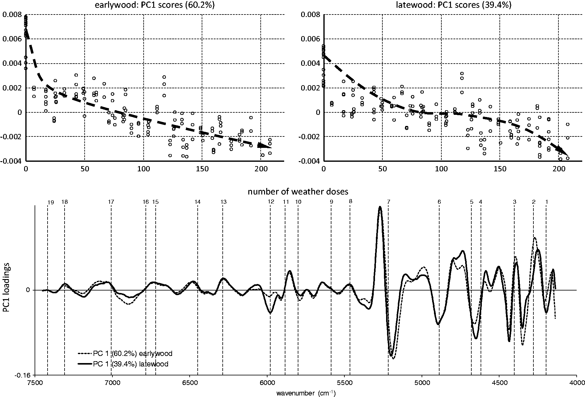

Conclusions

The goal of this work was to understand the mechanisms of aesthetic appearance alterations and chemical changes of untreated larch wood due to artificial weathering. Our hypothesis was that earlywood and latewood might show different dose–response behaviours, which could be evidenced with different sensors. The colour changes follow a degradation curve with a peak at ∼ 50 doses (weathering cycles) in the CIE a* and CIE b* values, both for earlywood and for latewood. Due to the particular shape (non-monotonic) of the curves representing colour coordinates, it was difficult to use these parameters for numerical modelling of the weathering dose. This difficulty was due to the fact that wood can appear to have similar values of CIE L*a*b* colour coordinates despite receiving different weathering doses. In this case, it becomes impossible to inversely link the dose with colour changes and to unambiguously predict number of doses received by means of the colour values.

Conversely, the degradation curve established for selected NIR bands (corresponding to functional groups of carbohydrates, extractives and lignin) was suitable to build a dose–response model linking wood degradation with the functional groups of wood polymers. In all cases, a clear trend in the absorbance value associated with increasing weathering dose was noticed. These curves, unlike the CIE L*a*b* values, are monotonic, meaning that each value of dose corresponds with only one value of NIR absorbance.

PCA of the NIR spectra further evidenced the clustering of the classes of doses, with the clear differentiation of the reference class. It was found that the discrimination between spectra at diverse cumulative weathering doses was more evident for earlywood than for latewood. This finding confirms the hypothesis that degradation kinetics differ, depending on the anatomical configuration of wood. The results of this study are highly useful for building a mathematical model that describes variation in the appearance of wood caused by weathering in a controlled experiment (known UV radiation and wetting time). It is a first step in establishing a universal dose–response model for natural weathering of wood. In the natural weathering case, precisely quantifying weathering parameters (determination of the weather dose) is much more challenging than in a fully controlled laboratory setting.