
Abstract
Randomized controlled trials in oncology often allow control group participants to switch to experimental treatments, a practice that, while often ethically necessary, complicates the accurate estimation of long-term treatment effects. When switching rates are high or sample sizes are limited, commonly used methods for treatment switching adjustment (such as the rank-preserving structural failure time model, inverse probability of censoring weights, and two-stage estimation) may produce imprecise estimates. Real-world data can be used to develop an external control arm for the randomized controlled trial, although this approach ignores evidence from trial subjects who did not switch and ignores evidence from the data obtained prior to switching for those subjects who did. This article introduces “augmented two-stage estimation” (ATSE), a method that combines data from non-switching participants in a randomized controlled trial with an external dataset, forming a “hybrid non-switching arm”. While aiming for more precise estimation, the augmented two-stage estimation requires strong assumptions. Namely, conditional on all the observed covariates: (1) a participant's decision to switch treatments must be independent of their post-progression survival, and (2) individuals from the randomized controlled trial and the external cohort must be exchangeable. With a simulation study, we evaluate the augmented two-stage estimation method's performance compared to two-stage estimation adjustment and an external control arm approach. Results indicate that performance is dependent on scenario characteristics, but when unconfounded external data are available, augmented two-stage estimation may result in less bias and improved precision compared to two-stage estimation and external control arm approaches. When external data are affected by unmeasured confounding, augmented two-stage estimation becomes prone to bias, but to a lesser extent compared to an external control arm approach.
Keywords
Introduction
Randomized controlled trials (RCTs) in clinical research often include the option for participants randomized to the control treatment (i.e. placebo or standard of care) to switch/crossover to the experimental treatment after a predefined time. This practice appears increasingly common in oncology and, from an ethical perspective, helps ensure that trial participants are not denied access to potentially beneficial new treatments. Allowing for treatment switching (also known as “crossover”) is also thought to improve recruitment/enrolment,1,2 (but see Chen and Prasad 3 who conclude otherwise). Unfortunately, treatment switching can complicate the estimation of overall survival (OS) benefits, as decision-makers are often interested in the hypothetical treatment effect of the experimental treatment versus the control treatment in jurisdictions where the experimental therapy is not yet available in the treatment pathway as a later line of therapy. 4
In oncology trials, where progression-free survival (PFS) is frequently the primary endpoint, treatment switching in the control group upon disease progression can obscure the estimation of OS—a key measure for reimbursement and health technology assessments (HTAs). To address these challenges, statistical adjustment methods have been proposed, such as rank-preserving structural failure time (RPSFT) models, 5 inverse probability of censoring (IPCW), 6 and two-stage estimation (TSE). 7 These approaches improve upon simple adjustment methods that simply censor subjects who switch treatments, given that switchers often have a different prognosis than non-switchers. However, these adjustment methods for treatment switching often result in highly uncertain estimates, especially in studies with a high rate of switching and/or a small sample size.
The National Institute for Health and Care Excellence (NICE) Decision Support Unit recently published a Technical Support Document (TSD 24, April 2024) that summarizes recommendations for adjusting survival time estimates in the presence of treatment switching in clinical trials. TSD 24 highlights the potential of using external data for treatment switching adjustment following similar calls in earlier work.8–10 However, until now, external data has only been used for treatment switching adjustment in select examples, where external evidence was used to (1) construct an external control arm (ECA) that was not impacted by switching and replace the RCT control arm considering alignment with the target trial population 11 ; (2) validate and select between different treatment switching adjustment methods (IPCW, TSE, and RPSFTM) 12 ; (3) estimate what post-progression survival (PPS) would have been in the RCTs had treatment switching not occurred. 13 This final example was the first to integrate external data into a TSE treatment switching adjustment model. 13 Although the Evidence Review Group report 14 raised concerns with regards to the use of external data in this case. Latimer and Abrams 15 noted that “the deliberations of the [NICE] Appraisal Committee regarding TA171 demonstrated openness to the use of external data in the presence of treatment switching.”
In this article, we propose an alternative way of using external data for treatment switching adjustment based on the concept of a “hybrid control arm.” Methods for hybrid-control arm studies are not new, but are only recently being considered in oncology research16,17 (e.g. using a control arm formed from historical clinical trials in metastatic colorectal cancer 18 or from EHR-derived data, such as the Flatiron Health database for advanced non-squamous non-small cell lung cancer (aNSCLC) 19 ). Our proposed augmented two-stage estimation (ATSE) method leverages a “hybrid non-switching arm” for comparison with the RCT switching arm, enabling more efficient estimation of survival beyond the switching time-point. We detail the ATSE method in Section 2, present a simulation study in Section 3, and conclude with a discussion in Section 4.
Methods
We begin by defining basic notation and summarizing the standard two-step estimation (TSE) procedure. We then describe the augmented TSE (ATSE), which uses a hybrid non-switching arm to estimate the effect of treatment switching on survival. Note that adjustment for treatment switching is typically needed when the switching patterns observed in the trial do not represent standard clinical practice; see TSD 24 for details. Also, treatment switching can take many forms (e.g. switches from the experimental group onto the control treatment, and switches from either randomized group onto other treatments). We focus exclusively on switches from the control group to the experimental treatment that do not represent standard clinical practice.
Notation
Let us begin by defining some useful notation; see Table 1 for a summary overview. Suppose subjects in the RCT are randomly allocated to either the “control arm” or the “treatment arm,” with the primary endpoint of interest being right-censored OS. Subjects who are randomized to the control are allowed to switch from the control to the experimental treatment following observed/confirmed disease progression, and we assume that any switches are likely to happen immediately or shortly following progression. Suppose also that patient-level data from an external cohort is available for subjects treated with the control who did not switch onto the experimental treatment. Finally, suppose a decision-maker is interested in evaluating the hypothetical OS benefit of the treatment versus the control in a jurisdiction where the experimental treatment is not available in subsequent lines of therapy.
Overview of notation.
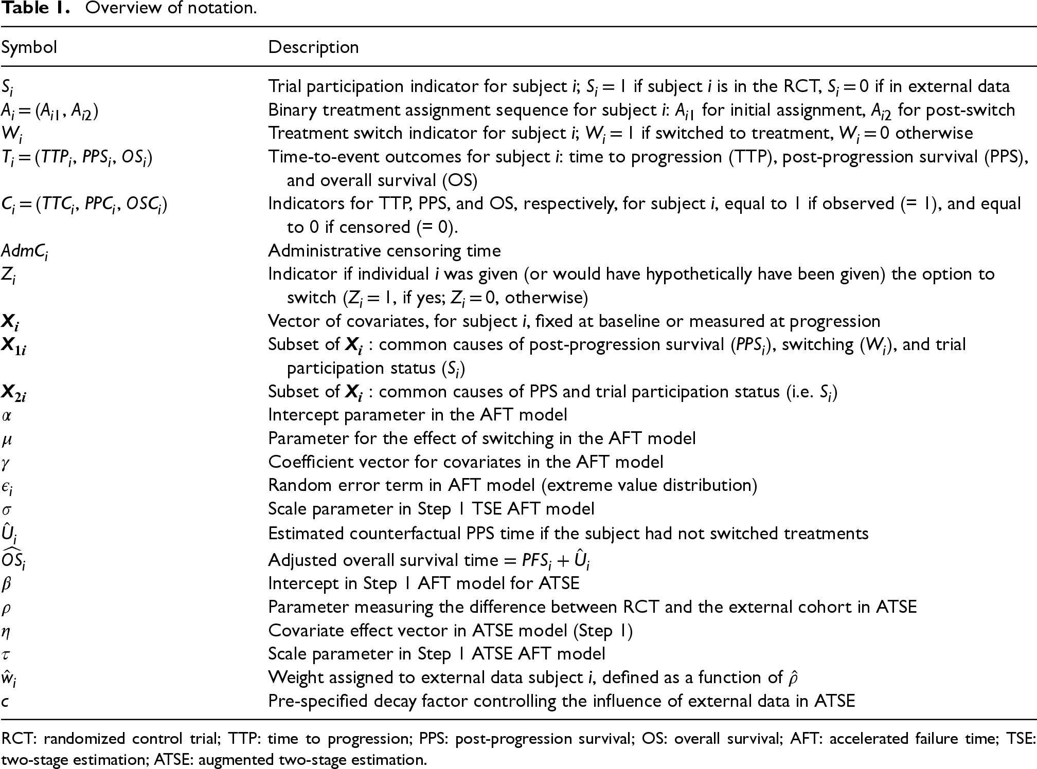
Overview of notation.
RCT: randomized control trial; TTP: time to progression; PPS: post-progression survival; OS: overall survival; AFT: accelerated failure time; TSE: two-stage estimation; ATSE: augmented two-stage estimation.
The i-th subject contributes Si, Ai = (A1i, A2i), Wi, Ti = (TTPi, PPSi, OSi), Ci = (TTCi, PPCi, OSCi), AdmCi, Zi, and
Let Zi = 1 indicate that individual i was given (or would hypothetically have been given) the option to switch (Zi = 0, otherwise). To be clear, if individual i was randomized to the control arm of the RCT (i.e. Si = 1 and Ai1 = 0), having a censored TTP (i.e. TTCi = 0) or an entirely unobserved TTP (i.e. TTPi = 0 and TTCi = 0) would indicate that this individual had no option to switch because they were presumably being followed closely and progression was never observed, so Zi = 0. However, if individual j was part of the external data (i.e. Sj = 0 and Aj1 = 0), having a censored TTP (i.e. TTCi = 0) or an entirely unobserved TTP (i.e. TTPi = 0 and TTCi = 0) might indicate that this patient was simply not being closely followed. It is important to think about the timepoint at which this patient would have hypothetically been given the option to switch to the experimental treatment had they been in the RCT and been followed more closely. If individual j's time of death is observed (i.e. OSCj = 1) and we assume Zj = 1, then, while their exact PPS is unknown, it will certainly be less than their time of death, and one could consider left-censoring (i.e. PPSj < (OSj−TTPj)).
Finally,
Overview of simulated scenarios.
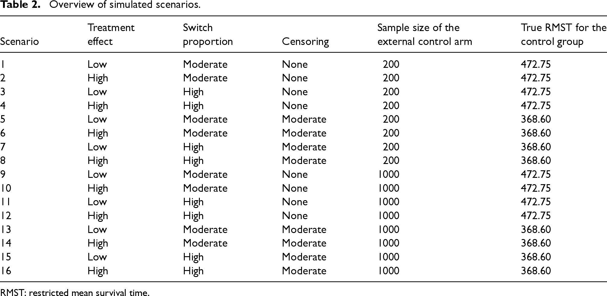
RMST: restricted mean survival time.
As its name suggests, the TSE approach for treatment switching adjustment involves two main steps. First, one estimates the effect of treatment switching on PPS. Then, in the second step, this effect estimate is used to estimate counterfactual survival times that would have been observed if switching had not occurred. In the first step, a standard parametric accelerated failure time (AFT) model (such as a Weibull model) is fit to all subjects randomized to the control arm of the RCT (with observed progression times), relating PPS to switching (W), and all possible confounders ( After obtaining parameter estimates from the AFT model, estimated counterfactual PPS times,
for the i-th subject (for all subjects for which Si = 1 and Ai1 = 0, and Zi = 1), where

for the i-th subject (for all subjects for which Si = 1 and Ai1 = 0, and Zi = 1); where 
Suppose, for example, that the effect of switching is to double the PPS (i.e. exp
After estimating the untreated survival times for patients who switched treatments (and conducting any necessary re-censoring), a new “adjusted RCT” dataset is created. This dataset combines observed OS times for patients who did not switch treatments with adjusted OS times for those who did. This adjusted RCT dataset can then be used to estimate the relative treatment effect with respect to OS. For example, a Cox proportional hazards model could be fit to estimate a treatment switching-adjusted hazard ratio (HR). Alternatively, the relative treatment effect could be estimated non-parametrically as a treatment switching-adjusted difference in restricted mean survival time (dRMST). Valid confidence intervals for these estimates can be obtained by bootstrapping the entire adjustment and estimation process. To be clear, bootstrapping allows one to account for the additional uncertainty involved in estimating the AF in Step 1.
Note that to obtain unbiased results, the TSE method relies on the assumption of “no unmeasured confounders.” This means that the Step 1 AFT model must include all variables that predict both PPS and treatment switching. In other words,
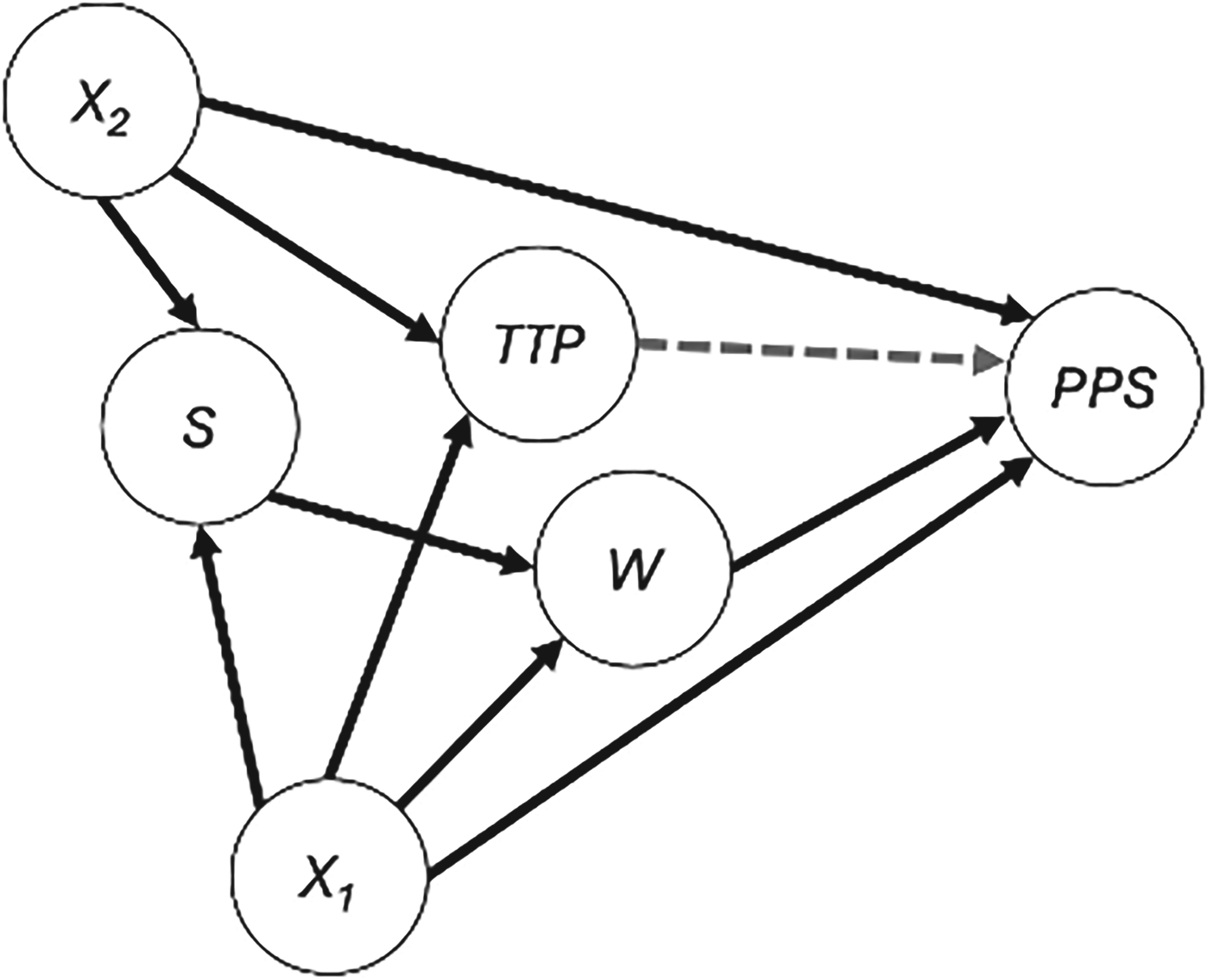
For estimating the effect of switching (W) on post-progression survival (PPS), there are two minimal sufficient adjustment sets: {S, X1} and {X1, X2}. The AFT model fit in Step 1 of the TSE is restricted to only those individuals with S = 1 (i.e. only subjects in the RCT) and must therefore include X1 (i.e. all variables that predict both PPS and treatment switching). The AFT model in Step 2 of the ATSE is fit to individuals from both the RCT (S = 1) and external data (S = 0) and must therefore include X1 and X2 (i.e. all variables that predict both PPS and treatment switching as well as all variables that predict both PPS and trial participation status).
The DAG in Figure 1 can be understood to illustrate the causal relationships between each of the variables. For instance, the arrow from
For TSE, a limited sample size in the non-switching subjects in the control arm of an RCT increases uncertainty in the estimation of the AF (i.e.
Various methods have been developed to construct the so-called “hybrid control arms,” whereby a trial's small control arm is combined with individuals from an external data source. These methods are mostly Bayesian approaches and include (modified) power prior models (Ibrahim and Chen 24 ), commensurate prior models (Hobbs et al. 25 ), and robust meta-analytic predictive prior (RMAPP) models (Schmidli et al. 26 ). Most recently, the Bayesian latent exchangeability prior (LEAP) model (Alt et al. 27 ) appears particularly promising (Campbell and Gustafson 28 ). However, since the TSE method is frequentist, for the ASTE we adopt the two-step dynamic borrowing approach recently proposed by Tan et al., 29 which reflects a frequentist analog to the modified power prior method.
The augmented TSE method consists of the following four steps. In the first step, a standard parametric AFT model (such as a Weibull model) is fit comparing the PPS between those randomized to the control arm who did not switch and those in the external control arm, adjusting for covariates
For example, a Weibull model could be specified such that:

Dynamic borrowing then considers the degree of dissimilarity in determining how much information to borrow from the external cohort. If the magnitude of 
To be clear, there are other options for the weight function defined in equation (4). Any function that is bounded between 0 and 1 and monotonically decreases weights with increasing The second step of the ATSE method is to fit a second AFT model to the weighted control subjects (i.e. all subjects with Ai1 = 0) with the weights defined from the previous step. This second AFT model relates PPS to switching (W), and includes covariates The third step of the ATSE approach is deriving the estimated counterfactual PPS times, The fourth and final step of the ATSE approach is to estimate the relative treatment effect of interest based on a new “adjusted RCT” dataset, which combines observed OS times for RCT patients who did not switch treatments with adjusted OS times for those RCT patients who did switch. For instance, a Cox proportional hazards model, or an AFT model, relating OS to treatment at randomization
for the i-th subject (for all subjects for which Ai1 = 0, and Zi = 1), where 
It is important to reiterate that, beyond the “no unmeasured confounders” assumption required in TSE (i.e. one must adjust for all variables that predict both PPS and treatment switching), the ATSE method requires an additional “no unmeasured confounders” assumption with respect to the external data. The DAG in Figure 1 illustrates that there are two minimal sufficient adjustment sets for estimating the effect of switching (W) on PPS: {S, X1} and {X1, X2}. The AFT model fit in Step 1 of the TSE is restricted to only those individuals with S = 1 (i.e. only subjects in the RCT) and must therefore include X1 (i.e., all variables that are common causes of PPS and W). The AFT model in Step 2 of the ATSE is fit to individuals from both the RCT (S = 1) and external data (S = 0) and must therefore include X1 and X2. Down-weighting the external data according to the suspected amount of unmeasured confounding as determined by the AFT model in Step 1 of the ATSE will help reduce the impact of confounding bias, but cannot entirely eliminate it. With regards to covariate selection, a conservative approach would be to adjust for all covariates that are considered important prognostic factors.
We have included
Objectives
To evaluate the performance of the ATSE method, we conducted a simulation study designed to mirror typical settings in clinical research with treatment switching and incorporation of external data. This simulation study aimed to assess the accuracy and robustness of the ATSE approach under various conditions, including variations in switching rates, and different decay factors for the ATSE hybrid arm. Here, we provide a summary of the data-generating mechanism, the estimand of interest, and the methods we compared according to various performance measures. The simulation study was conducted using R. The code used to simulate the data is provided in the Supplementary Material.
Data generation and mechanism
We followed the data generation procedure used outlined by Latimer et al. 31 for their eight “simple scenarios” with a few modifications. Specifically, we simulated RCT datasets with a sample size of NRCT = 500 and 2:1 randomization in favor of the experimental group, and with treatment switching permitted from the control group to the experimental treatment following progression.
OS times were simulated based on a two-component mixture Weibull baseline survival function and were dependent on three binary variables: treatment, prognosis 
TTP times were simulated as a function of OS times, so that on average, an individual's TTP was one-third of their OS. More specifically, TTP times were equal to OS times multiplied by a random draw from a beta(5, 10) distribution. A short delay was assumed between an individual's true progression time and their observed progression time by setting the observed progression time as equal to their first “visit time” following the progression event, with “visits” simulated every 21 days from randomization to death.
We simulated external control datasets in the same way that the RCT datasets were simulated, but with
Sixteen scenarios were simulated varying (1) the magnitude of the treatment effect, (2) the degree of switching, (3) the censoring, and (4) the sample size of the external control arm; see Table 2. These scenarios were based on Latimer et al.’s
31
eight simple scenarios. Specifically, for scenarios with “low treatment effect,” we set
To investigate the impact of unmeasured confounding, for each of the sixteen scenarios, 2000 datasets were simulated with three different conditions. In Condition A (“Complete”) there was no unmeasured confounding, meaning the unmeasured prognostic factor U did not impact the probability of switching and had the same distribution in the RCT and external control (i.e. all subjects in the RCT and external control,
As in Latimer et al., 31 the estimand of interest for the simulation study was the restricted mean survival time (RMST) in the control group at study end-date (5000 days for Scenarios 1–4 and 9–12; 546 days for Scenarios 5–8 and 13–16). The true RMST value in the control group was 472.75 days in Scenarios 1–4 and 9–12, and was 368.6 days in Scenarios 5–8 and 13–16, based on numerical integration.
When extrapolation was required to calculate the RMST, we used a flexible Royston-Parmar parametric splines model with three knots (using the RMST R package; https://github.com/scientific-computing-solutions/RMST), consistent with HTA recommendations. 32
Methods to be compared
We compared the following methods: Oracle: A standard ITT analysis undertaken on the simulated data prior to simulating the impact of switching, which represents the “truth” for each simulation. ITT: A standard ITT analysis on the simulated data after switching impacted the outcomes. TSE: Treatment switching-adjusted analysis using TSE based on only the RCT data with re-censoring applied (Section 2.2). ECA: A propensity-score-based analysis in which the external control data is used as an external control arm (and individuals randomized to control in the RCT are ignored). Specifically, we used the “weightit” function from the WeightIt R library
33
to derive the average treatment effect for the treated (ATT) weights using a logistic regression model. The weighted OS ECA data was then used to estimate the RMST in the control group. ATSE (c = 1): An analysis based on the proposed approach with decay factor set to c = 1 and re-censoring applied (Section 2.3). This smaller value of c will result in borrowing more information from the external data. ATSE (c = 4): An analysis based on the proposed approach with decay factor set to c = 4 and re-censoring applied (Section 2.3). This method considers a “mid-range” value of c. ATSE (c = 8): An analysis based on the proposed approach with decay factor set to c = 8 and re-censoring applied (Section 2.3). This larger value of c will result in borrowing less information from the external data. ATSE (c = 4) with adjustment for TTP: An analysis based on the proposed approach with decay factor set to c = 4 and re-censoring applied (Section 2.3), which includes TTP as a covariate in the ATSE Step 1 and Step 2 AFT models.
Performance measures
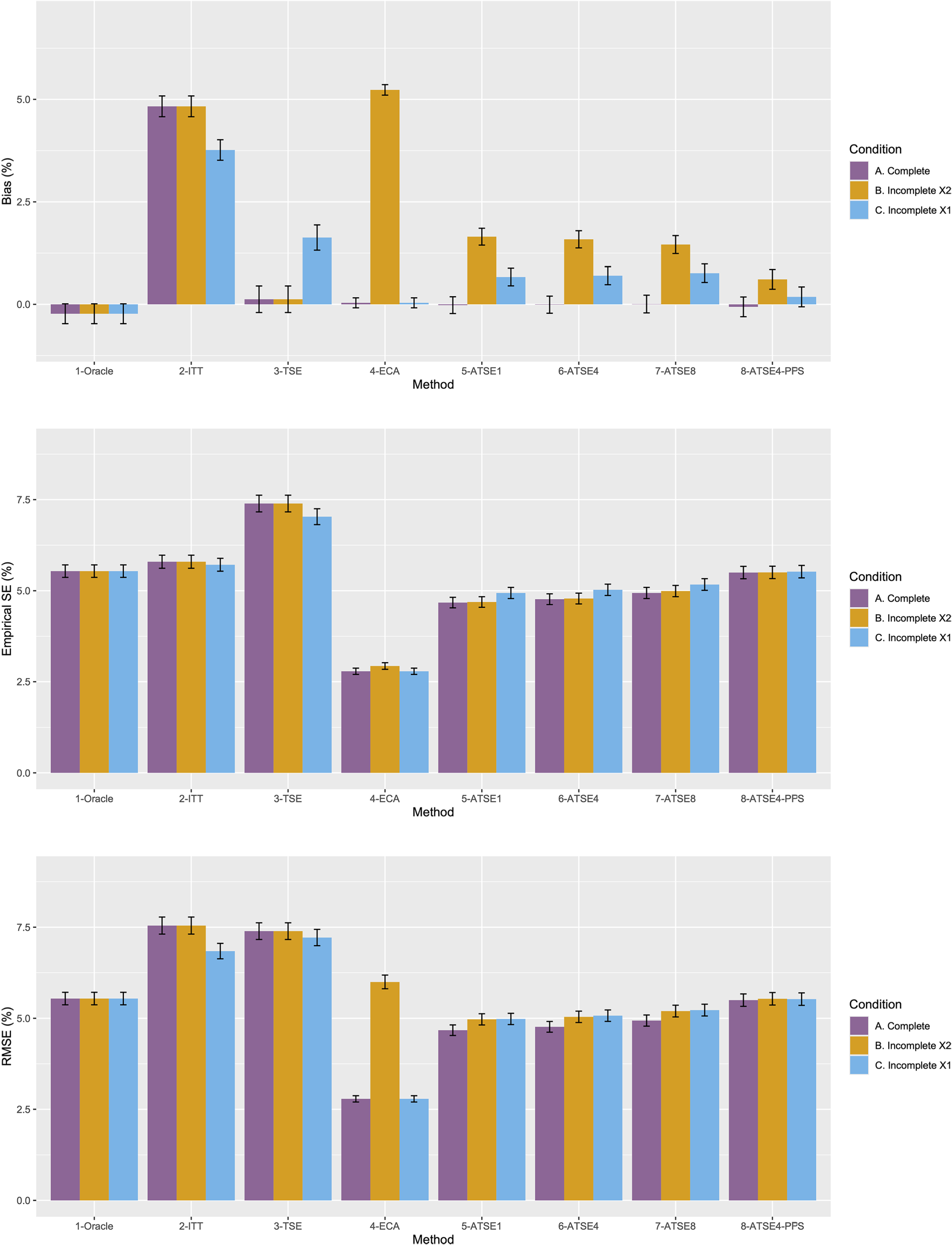
Consistent with Latimer et al., 31 the performance of each method was evaluated according to the percentage bias in the estimate of the control group RMST at the study end date. Percentage bias was estimated by taking the difference between the estimated RMST and the true RMST, expressed as a percentage of the true RMST. Root mean squared error (RMSE) and empirical standard errors (SEs) of the RMST estimates were also calculated for each method and expressed as percentages of the true RMST.
Results
Figure 2 plots the results for Scenario 1 and Figure 3 plots the results for Scenario 9. Figures 4 to 9 display results in nested loop plots for the percentage bias and empirical SE across all 16 scenarios. Tables 3 to 6 in the Appendix list the complete results. The simulation study provided very accurate estimates. For the mean RMST percentage bias, the Monte Carlo SE (MCSE) never exceeding 0.20% across all 16 scenarios. For the empirical SE as a percentage of true RMST, the maximum (across all 16 scenarios) MCSE was 0.14% and for the RMSE as a percentage of true RMST, the maximum MCSE was 0.34%. Error bars plotted in Figures 2 and 3 correspond to ±1.96 times the MCSE. Finally, the differences between Figures 2 and 3 for the Oracle, ITT, and TSE methods provide an additional measure of the size of the Monte Carlo error (since, in the absence of Monte Carlo error, these should be identical).
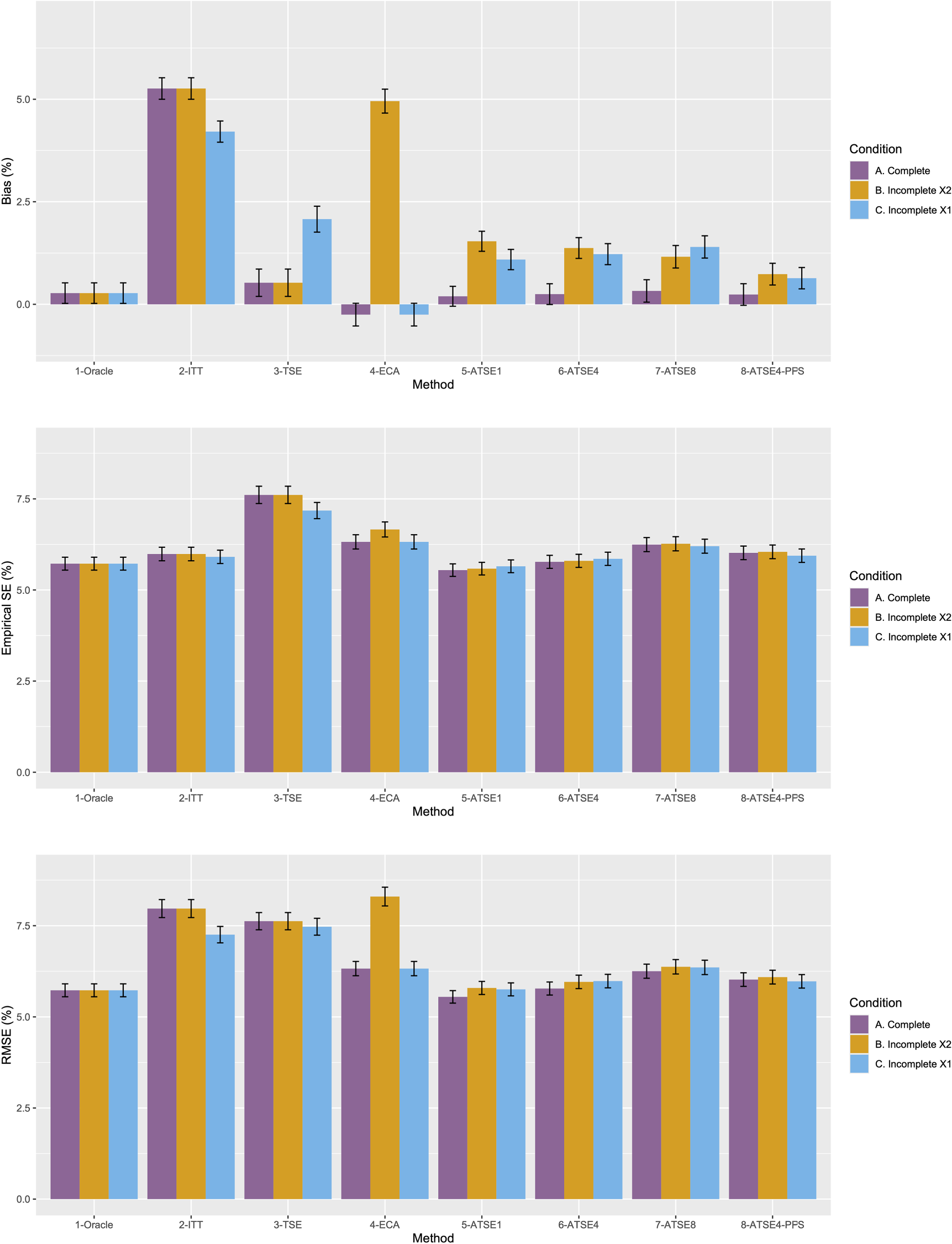
Simulation study results from Scenario 1.
Simulation study results from Scenario 9.
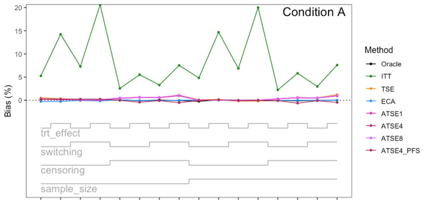
Simulation study results: Percentage bias for Condition A (“Complete”) across the 16 scenarios.
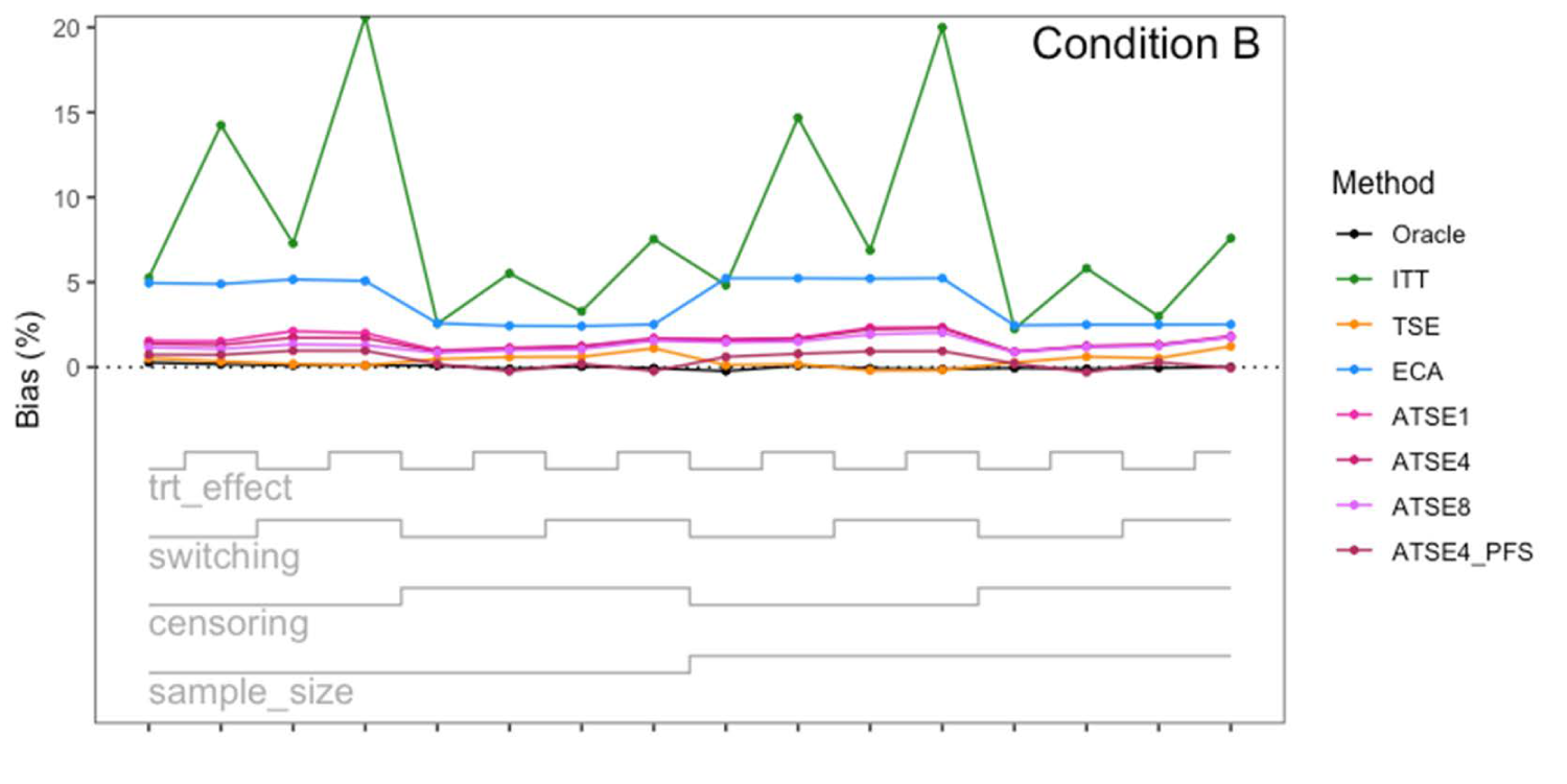
Simulation study results: Percentage bias for Condition B (“Incomplete X2”) across the 16 scenarios.
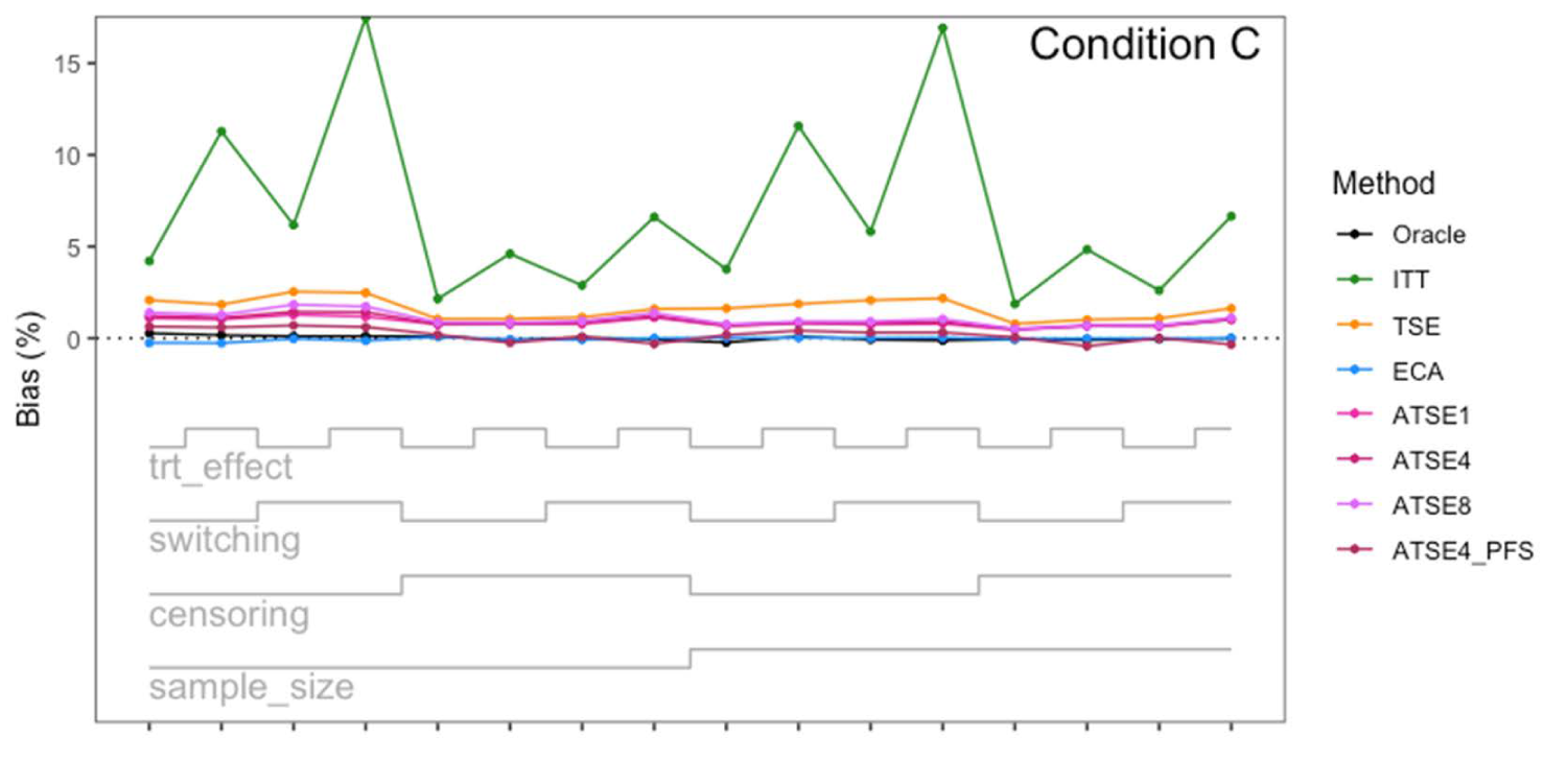
Simulation study results: Percentage bias for Condition C (“Incomplete X1”) across the 16 scenarios.
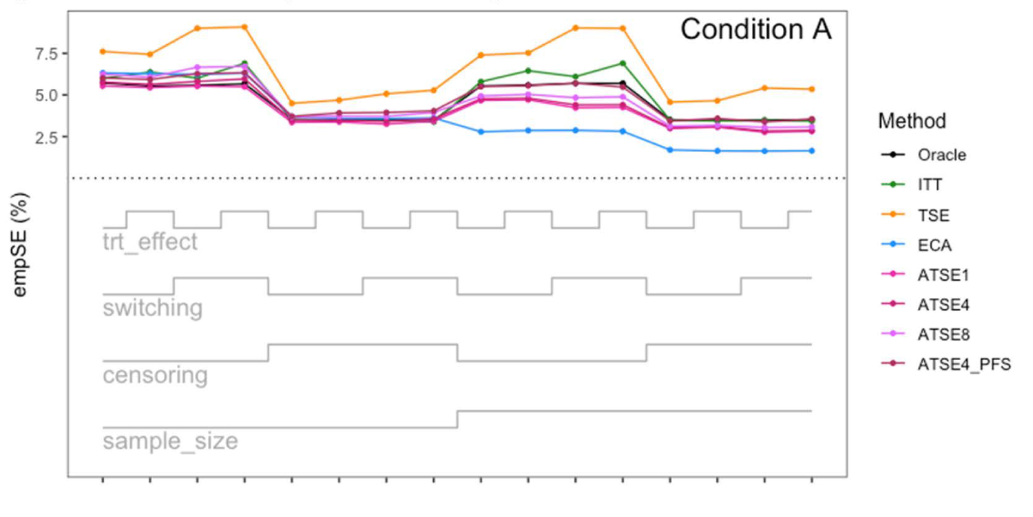
Simulation study results: Empirical SE for Condition A (“Complete”) across the 16 scenarios.
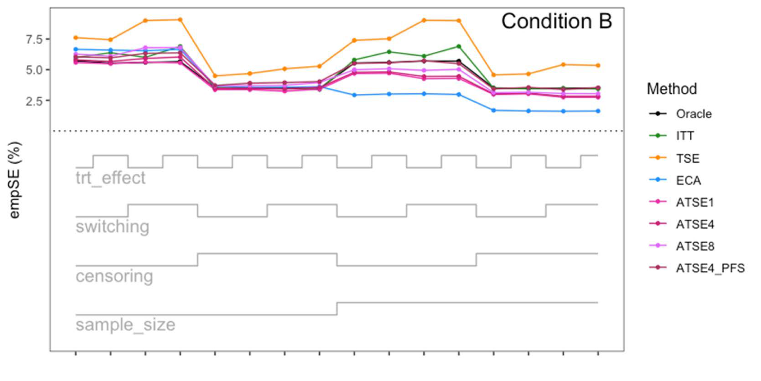
Simulation study results: Empirical SE for Condition B (“Incomplete X2”) across the 16 scenarios.
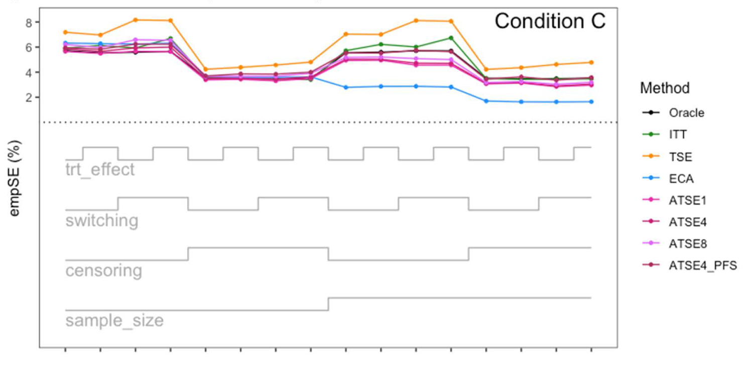
Simulation study results: Empirical SE for Condition C (“Incomplete X1”) across the 16 scenarios.
Let us focus first on the results from Scenario 1. As expected, under all three conditions, the ITT analysis over-estimates the control group RMST, resulting in a percentage bias of between 4.4% and 5.4%. Under Condition A (“Complete”), all other methods (TSE, ECA, and ATSE) predict the control group RMST with negligible bias (<= 0.6%). Among these other methods, the ASTE analysis appeared to be the most efficient with SEs ranging from 5.4% to 6.2%. Notably, the ECA approach had an empirical standard error of 6.3%, lower than the TSE, which had an empirical standard error of 7.6%. It is interesting that the SE for the ATSE can be slightly lower than for the Oracle (compare 5.4% to 5.7%). This can be explained by the fact that more data is being used in the ATSE analysis. Under Condition B (“Incomplete X2”), when there may be confounding bias with respect to the external control data, the ECA appears to be biased, over-estimating the control group RMST by 5.0%. The ATSE analyses are also biased, but to a much lesser degree, over-estimating the control group RMST by only 1.2%–1.6%. Under Condition C (“Incomplete X1”), when there may be confounding bias with respect to the treatment switching adjustment, the TSE appears to be biased, over-estimating the control group RMST by about 2.2%. The ATSE analyses are also biased, over-estimating the control group RMST by about 1.2%–1.5%. Results were similar across all scenarios.
The impact of using different values for the decay factor with ATSE was, overall, rather minimal. Recall that a smaller decay factor corresponds to a higher degree of borrowing from the external data. We see that under Condition A (“Complete”), the empirical SE as a percentage of the true RMST is smallest when c = 1 and is highest when c = 8, meaning that more borrowing leads to more efficiency. Under Condition B (“Incomplete X2”), where the external control data introduces bias, the percent bias in RMST is highest when c = 1, and is lowest when c = 8. In contrast, under Condition C (“Incomplete X1”), the percent bias in RMST is lowest when c = 1, and is highest when c = 8. As such, the decay factor seems to correspond to a trade-off between the potential bias due to unmeasured confounding in either the RCT treatment switching-adjusted controls or the external control.
The impact of adjusting for TTP in the ASTE was notable. We see that the degree of bias due to confounding is substantially reduced at the cost of a modest increase in SE. We do not observe any substantial impact with respect to differing treatment effect sizes (
The TSD 24 specifically brings attention to the potential for “external data [is used] to estimate counterfactual survival beyond the switching time-point” and suggests that “further research [to develop such methods] may be valuable” (TSD 24, April 2024). In this article, we proposed a new approach, the ATSE, which may indeed be prove valuable.
While RWE can be used as an external control arm to completely replace a crossover contaminated RCT control arm, this strategy discards a large amount of potentially valuable data (including the TTP times of those RCT subjects randomized to control) and can be susceptible to bias due to unmeasured confounding. 34 As illustrated in the simulation study, the ATSE approach leverages all the available data (and only the necessary external data) and consequently may be less impacted by confounding bias. This aligns with the current understanding that hybrid control arm studies (also known as “augmented RCTs”) should be considered a higher level of evidence than external control arm studies; see Gray et al. 35
If the assumptions underlying the treatment switching adjustment are suspect or the size of the external dataset is very large, then the ECA may be preferable to the ATSE approach. Alternatively, if the assumption of exchangeability for the subjects in the external data is suspect, then the TSE may be preferable to the ATSE approach. Another issue to consider is the possibility of immortal time bias and selection bias. To avoid immortal time bias and selection bias with the ECA approach, one must carefully select an appropriate “time-zero.” This can often be challenging (Jaksa et al., 23 Fu et al., 36 and Hernán et al. 37 ). With the proposed ATSE approach, selecting the appropriate “time-zero” should be relatively straightforward so long as the progression time is well defined. Figure 10 illustrates where the different methods might fit in terms of deciding upon the most appropriate approach.
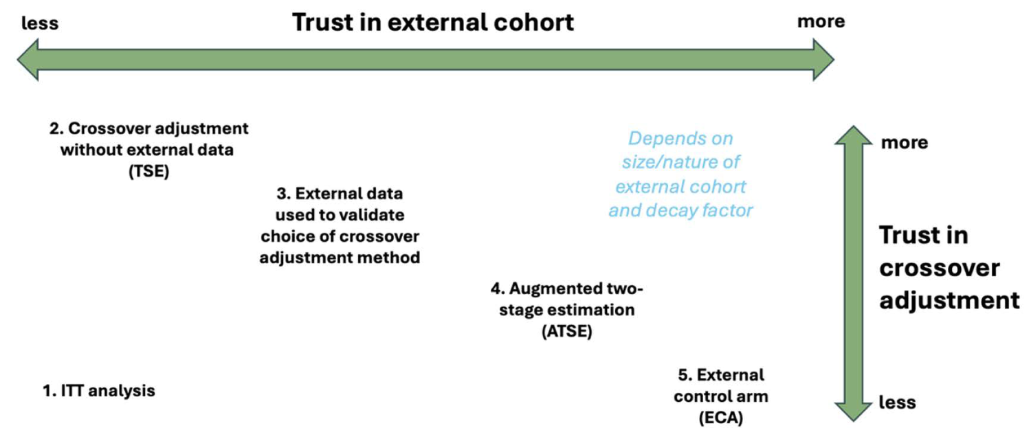
If the assumptions underlying the treatment switching adjustment are suspect, then the ECA may be preferable to the ATSE approach. Alternatively, if the assumption of exchangeability for the subjects in the external data is suspect, then the TSE may be preferable to the ATSE approach. If no assumptions can be relied upon, the ITT analysis (while biased) will be most appropriate.
When compared to the standard TSE approach, the ATSE approach has potential to obtain more precise estimation of survival outcomes particularly when sample sizes are small, and switching rates are high. However, the need for strong assumptions remains. With TSE, the assumption of no unmeasured confounding implies that, conditional on all the observed covariates, a participant's decision to switch is independent of their PPS. With ATSE, an additional assumption is also required: Conditional on all observed covariates, individuals from the RCT and the external cohort must be exchangeable; see Bours.
38
The ATSE method also requires one to pre-specify a value for the decay factor, which will impact the overall amount of borrowing. Tan et al. recommend that this value be determined prior to analyzing the data by means of a simulation study, and based on Tan et al.'s simulation study, Sengupta et al.
19
use a value of
While the ATSE method represents a promising avenue for addressing treatment switching in clinical trials, its limitations must be acknowledged and carefully considered. One notable limitation is the assumption that treatment switching occurs exclusively at, or shortly after, disease progression. This assumption may not always hold true in real-world scenarios, where switching can occur for various reasons and at different points in time. Our simulation study was simply intended to demonstrate a proof of concept in simple scenarios, and as such, we did not investigate the impact of time-dependent confounding. The g-computation TSE method, proposed by Latimer et al., 31 offers a potential solution for situations where switching is not confined to the point of progression (or to another well-defined “secondary baseline”). More recently, Jackson et al. have proposed a variety of new approaches for TSE and suggest a method in which the secondary baseline is defined as the time of an individual's first subsequent treatment. Further research and simulation studies are needed to explore the feasibility of augmenting the g-computation TSE and other TSE approaches with external data. Our simulation study was also rather simplistic in that we simulated TTP times as being equal to (on average) about one-third of OS times. Future simulation studies could instead consider multi-state models (Jansen et al. 39 ).
Another potential limitation of ASTE might be the need for comprehensive data on all confounding variables. To avoid any bias due to unmeasured confounding, one must adjust for any factors that could simultaneously influence survival, switching, and participation in the RCT vs external cohorts. Identifying these factors could prove difficult, and the conservative approach of simply adjusting for all variables that could be considered important prognostic factors requires substantial data availability. The dynamic borrowing approach we propose within the ATSE method can help reduce the amount of bias due to unmeasured confounding, but cannot entirely eliminate it. Adjusting for TTP as a “proxy confounder” might help further mitigate the risk of bias due to unmeasured confounding. Finally, to calculate PPS for individuals in the external data, we emphasize that accurate recording of TTP is important and acknowledge that cancer progression is often poorly recorded in both hospital and registration data.40,41
Supplemental Material
sj-docx-1-smm-10.1177_09622802251374838 - Supplemental material for Augmented two-stage estimation for treatment switching in oncology trials: Leveraging external data for improved precision
Supplemental material, sj-docx-1-smm-10.1177_09622802251374838 for Augmented two-stage estimation for treatment switching in oncology trials: Leveraging external data for improved precision by Harlan Campbell, Nicholas Latimer, Jeroen P Jansen and Shannon Cope in Statistical Methods in Medical Research
Footnotes
Acknowledgements
The research was performed without specific funding.
Ethical approval and informed consent statements
There are no human participants in this article, and informed consent is not required.
Funding
The authors received no financial support for the research, authorship, and/or publication of this article.
Declaration of conflicting interests
The author(s) declared the following potential conflicts of interest with respect to the research, authorship, and/or publication of this article: Harlan Campbell, Jeroen P Jansen, and Shannon Cope are employees of Precision AQ.
Data availability statement
The data that support the findings of this study are simulated data, and the code used to simulate this data is available in the Appendix. Additional code is available from the corresponding author upon reasonable request.
Supplemental material
Supplemental material for this article is available online.
Notes
References
Supplementary Material
Please find the following supplemental material available below.
For Open Access articles published under a Creative Commons License, all supplemental material carries the same license as the article it is associated with.
For non-Open Access articles published, all supplemental material carries a non-exclusive license, and permission requests for re-use of supplemental material or any part of supplemental material shall be sent directly to the copyright owner as specified in the copyright notice associated with the article.