Sage Journals: Discover world-class research

Abstract

In oncology trials, control group patients often switch onto the experimental treatment during follow-up, usually after disease progression. In this case, an intention-to-treat analysis will not address the policy question of interest – that of whether the new treatment represents an effective and cost-effective use of health care resources, compared to the standard treatment. Rank preserving structural failure time models (RPSFTM), inverse probability of censoring weights (IPCW) and two-stage estimation (TSE) have often been used to adjust for switching to inform treatment reimbursement policy decisions. TSE has been applied using a simple approach (TSEsimp), assuming no time-dependent confounding between the time of disease progression and the time of switch. This is problematic if there is a delay between progression and switch. In this paper we introduce TSEgest, which uses structural nested models and g-estimation to account for time-dependent confounding, and compare it to TSEsimp, RPSFTM and IPCW. We simulated scenarios where control group patients could switch onto the experimental treatment with and without time-dependent confounding being present. We varied switching proportions, treatment effects and censoring proportions. We assessed adjustment methods according to their estimation of control group restricted mean survival times that would have been observed in the absence of switching. All methods performed well in scenarios with no time-dependent confounding. TSEgest and RPSFTM continued to perform well in scenarios with time-dependent confounding, but TSEsimp resulted in substantial bias. IPCW also performed well in scenarios with time-dependent confounding, except when inverse probability weights were high in relation to the size of the group being subjected to weighting, which occurred when there was a combination of modest sample size and high switching proportions. TSEgest represents a useful addition to the collection of methods that may be used to adjust for treatment switching in trials in order to address policy-relevant questions.

Keywords

Treatment switching treatment crossover survival analysis overall survival oncology health technology assessment time-to-event outcomes prediction time-dependent confounding structural nested models g-estimation counterfactual

1 Introduction

In recent times there has been considerable interest in methods that allow treatment effects to be estimated adjusting for treatment changes that occur in randomised controlled trials (RCTs).^1–7 Treatment pathways observed in RCTs often do not reflect those that would be observed in reality, and therefore intention to treat (ITT) analyses may not address the question of interest. For instance, in clinical trials of new oncology therapies, patients who are randomised to the control group are often permitted to switch onto the experimental treatment during the trial, usually after disease progression. In such circumstances, the ITT analysis provides an estimate of the effect of immediate compared to deferred experimental treatment. An alternative estimand might consider the effectiveness of immediate experimental treatment compared to no experimental treatment. This is particularly important in health technology assessment (HTA), where the objective is usually to identify whether inserting a new treatment into the treatment pathway at the line of therapy designated by its licence represents an effective and cost-effective use of healthcare resources, compared to retaining the existing treatment pathway. In HTA, treatment benefits are usually summarised using estimates of mean (quality adjusted) survival advantages.^8–11

Treatment changes are to be expected in any clinical trial. If these changes reflect what would happen in practice, it is not necessary to make adjustments to enable appropriate HTA decision making. However, switching from the control group onto the experimental treatment does cause a problem. If the HTA decision maker does not recommend a new treatment it will not be available in the health system. The HTA decision problem involves a comparison of a world in which the new treatment exists (and is given at its licensed line of therapy) to a world in which the new treatment does not exist at all. Therefore, if patients randomised to the control group of an RCT are permitted to receive the experimental treatment at some point during the trial, the observed treatment pathway is not relevant for the HTA decision problem.

This is illustrated in Figure 1. The horizontal axis represents survival time, consisting of progression-free survival (PFS) and post-progression survival (PPS). Rows 1 and 2 illustrate what we would ideally observe in an RCT. Row 1 (the upper row) illustrates survival in the control group in the absence of any switching onto the experimental treatment, and Row 2 (the middle row) illustrates survival in the experimental group. However, when control group patients are permitted to switch onto the experimental treatment at the point of disease progression, we observe Row 3 (the bottom row) and not Row 1. If switching occurs, an ITT analysis provides an estimate of the difference between Row 2 and Row 3. In contrast, the HTA decision maker is likely to require an estimate of the difference between Row 2 and Row 1 – comparing a world where the experimental treatment exists to one where it does not. Therefore, the ITT analysis does not address the HTA decision problem; an analysis that adjusts for treatment switching is needed such that Row 2 can be compared to an estimated Row 1.

Figure 1.

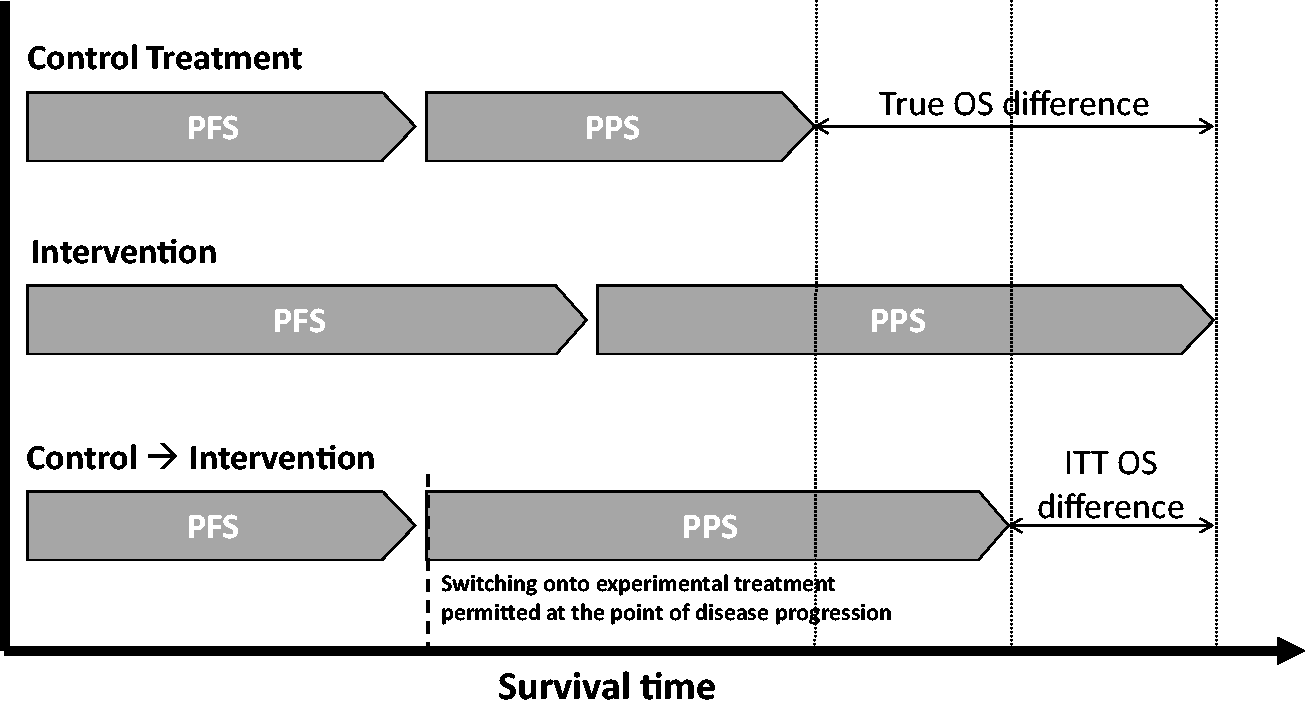
Illustrating treatment switching – switching immediately upon disease progression. PFS: progression-free survival; PPS: post-progression survival; OS: overall survival; ITT: intention-to-treat.Adapted from [1] with permission of SAGE publications.

Research on methods for adjusting for treatment switching in an RCT context have focussed on rank preserving structural failure time models (RPSFTM), inverse probability of censoring weights (IPCW) and two-stage estimation (TSE).^{1–7,12–14} These methods have been included in analyses used to make reimbursement decisions on new cancer drugs around the world.⁵ When attempting to adjust analyses to account for treatment switches that occur over time, the key difficulty is time-dependent confounding.¹⁵ If a variable influences the treatment switch decision, is prognostic for the outcome of interest (such as survival), and is itself affected by treatment, it is a time-dependent confounder for the effect of treatment on outcome. The RPSFTM and IPCW approaches originate in the causal inference literature and, provided their assumptions hold, are able to provide unbiased adjusted treatment effects in the presence of time-dependent confounding.^16–18 In contrast, the TSE method uses a simple estimation procedure and is only appropriate when switching occurs after a specific disease-related time-point, referred to as a “secondary baseline”, such as disease progression.¹² The first stage of the method requires the post-secondary-baseline treatment effect in switchers to be estimated, but the method does not adjust for any time-dependent confounding that may occur between the secondary baseline and the time of switch. This may be reasonable when switching occurs either at or very soon after the secondary baseline (as depicted in Figure 1), but if there is an appreciable gap between the secondary baseline and the time of switch (as depicted in Figure 2), the TSE method may become biased.

Figure 2.

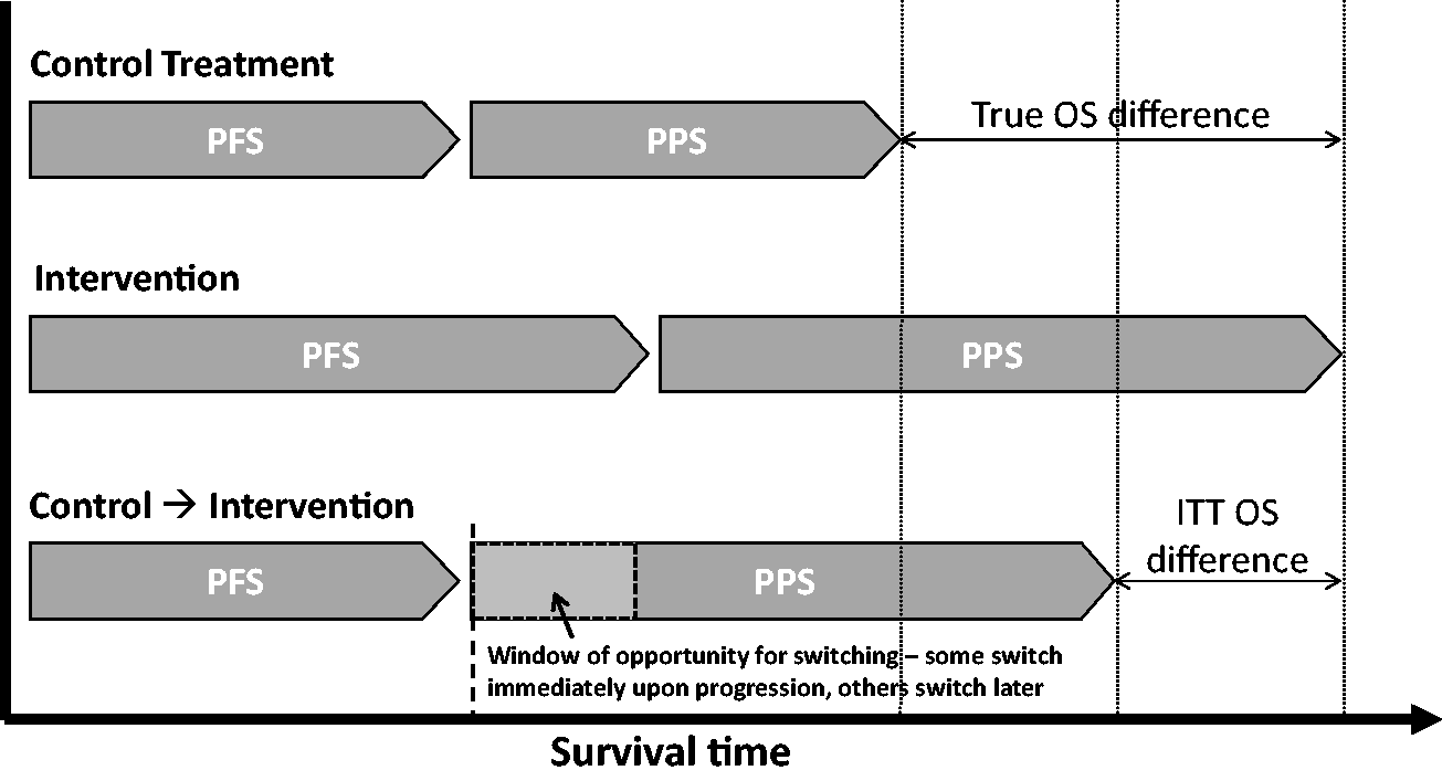
Illustrating treatment switching – switching sometime after disease progression. PFS: progression-free survival; PPS: post-progression survival; OS: overall survival; ITT: intention-to-treat.

To illustrate this, first consider a simple case where switching can only occur immediately upon disease progression. Consider an RCT investigating the effectiveness of an experimental adjuvant treatment for non-metastatic cancer, in which switching from the control group onto the experimental treatment is permitted at the point of disease progression. The TSE method would estimate the effect of switching by comparing post-progression survival in control group switchers and non-switchers, adjusting for differences between switchers and non-switchers at the point of disease progression. The directed acyclic graph (DAG)¹⁹ presented in Figure 3 illustrates the post-progression period for control group patients in this example. Upon disease progression, the decision as to whether or not a patient switches treatment (denoted by $S_{1}$ in Figure 3) is dependent on prognostic characteristics measured either at or before the time of disease progression (labelled $V_{0}$ in Figure 3). Let us assume that receiving treatment prolongs survival (Y) and affects the probability of metastatic disease developing at a later time-point ( $M_{2}$ in Figure 3). Note that in this example (and throughout this paper), we consider a case where disease progression is distinct from metastatic disease – first, disease progression may occur (as measured, for example, by an increase in tumour size) and subsequently the disease may become metastatic. $S_{1}$ has a direct effect on Y, and also an indirect effect through $M_{2}$ . In this case, an analyst using the TSE method to estimate the effect of $S_{1}$ on Y can simply adjust for $V_{0}$ . $M_{2}$ is not a confounder because it is not a cause of $S_{1}$ and therefore does not need to be adjusted for in the analysis.

Figure 3.

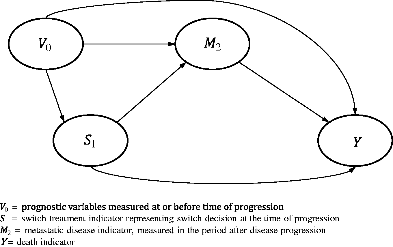
Directed acyclic graph illustrating post-progression switching with no time-dependent confounding.

Next, consider a more complex case, where switching can occur either at the point of disease progression or at an additional time-point thereafter ( $S_{2}$ ). The DAG presented in Figure 4 illustrates the post-progression period for control group patients in this case. Upon disease progression, the decision as to whether or not a patient switches treatment ( $S_{1})$ is again dependent on prognostic characteristics measured at or before the time of disease progression ( $V_{0}$ ). Again receiving treatment prolongs survival (Y) and affects the probability of metastatic disease developing at a later time-point ( $M_{2}$ ) but in this case developing metastatic disease affects the clinician’s decision as to whether or not a patient should subsequently change treatments ( $S_{2}$ ). In this case, an analyst using the TSE method to estimate the effect of switching must decide whether to include the occurrence of metastatic disease ( $M_{2}$ ) as a time-varying covariate in their statistical model. If they do not, the estimate of the treatment effect will be biased because patients who switch treatment have a different prognosis to those who do not switch – this is known as confounding by indication,¹⁵ and in Figure 4 is illustrated by the open backdoor path from $S_{2} \leftarrow M_{2} \to Y$ . However, including metastatic disease as a time-varying covariate will also result in biased estimates of the treatment effect because part of the treatment effect occurs through reducing the likelihood of metastatic disease (the causal path from $S_{1} \to M_{2} \to Y$ would be blocked). In this example, $M_{2}$ is a time-dependent confounder. The TSE method would produce biased estimates of the treatment effect because simple regression adjustment cannot deal with time-dependent confounders.

Figure 4.

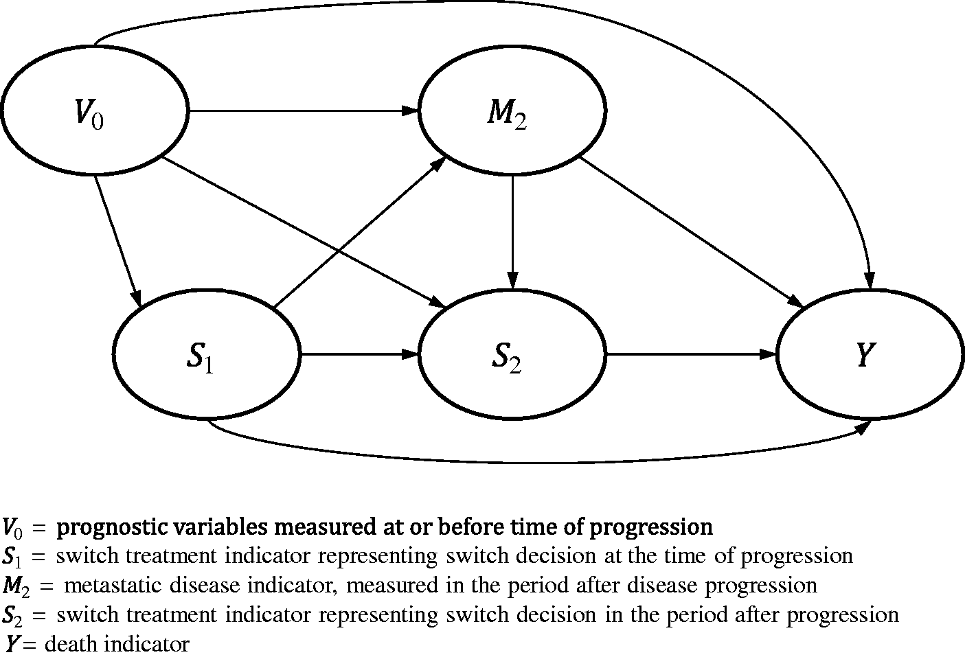
Directed acyclic graph illustrating post-progression switching with time-dependent confounding.

It is possible to apply the TSE method using a more sophisticated estimation procedure (g-estimation) in order to obtain unbiased estimates in the presence of time-dependent confounding. Previous research attempted to assess such a technique, but found that it did not work well in realistic simulated scenarios – the method often failed to converge and frequently resulted in high levels of bias.¹² In this paper, we re-visit this. We improved the statistical program used to apply the method (stgest, for use in Stata²⁰) – principally by improving the g-estimation algorithm used – and tested this in a simulation study including scenarios with and without time-dependent confounding. Our aims were to develop and assess a version of the TSE method that is capable of adjusting for time-dependent confounding and to compare this to alternative adjustment methods in a range of scenarios. We focus on the problem typically seen in HTA,^1–7,21,22 whereby a subset of control group patients switch onto the experimental treatment after disease progression and we wish to estimate what survival would have been in the control group as a whole if this switching had not occurred.

2 Methods

In this section, we first describe the TSE method using simple estimation (denoted TSEsimp) and using g-estimation (TSEgest). We also summarise RPSFTM and IPCW, because these represent relevant comparator methods that can control for time-dependent confounding. We then describe the design of our simulation study.

2.1 Adjustment methods

Box 1 summarises the key assumptions used by each of the adjustment methods, in our context. We assume that switching is not a problem in the experimental group (that is, we only address switches from the control group onto the experimental treatment, not switches in the opposite direction). Below we provide more detail on each adjustment method, organised by concept, assumptions and modelling approach. Box 1

Key assumptions of TSEsimp, TSEgest, IPCW and RPSFTM for estimating unbiased treatment effects in the presence of treatment switching.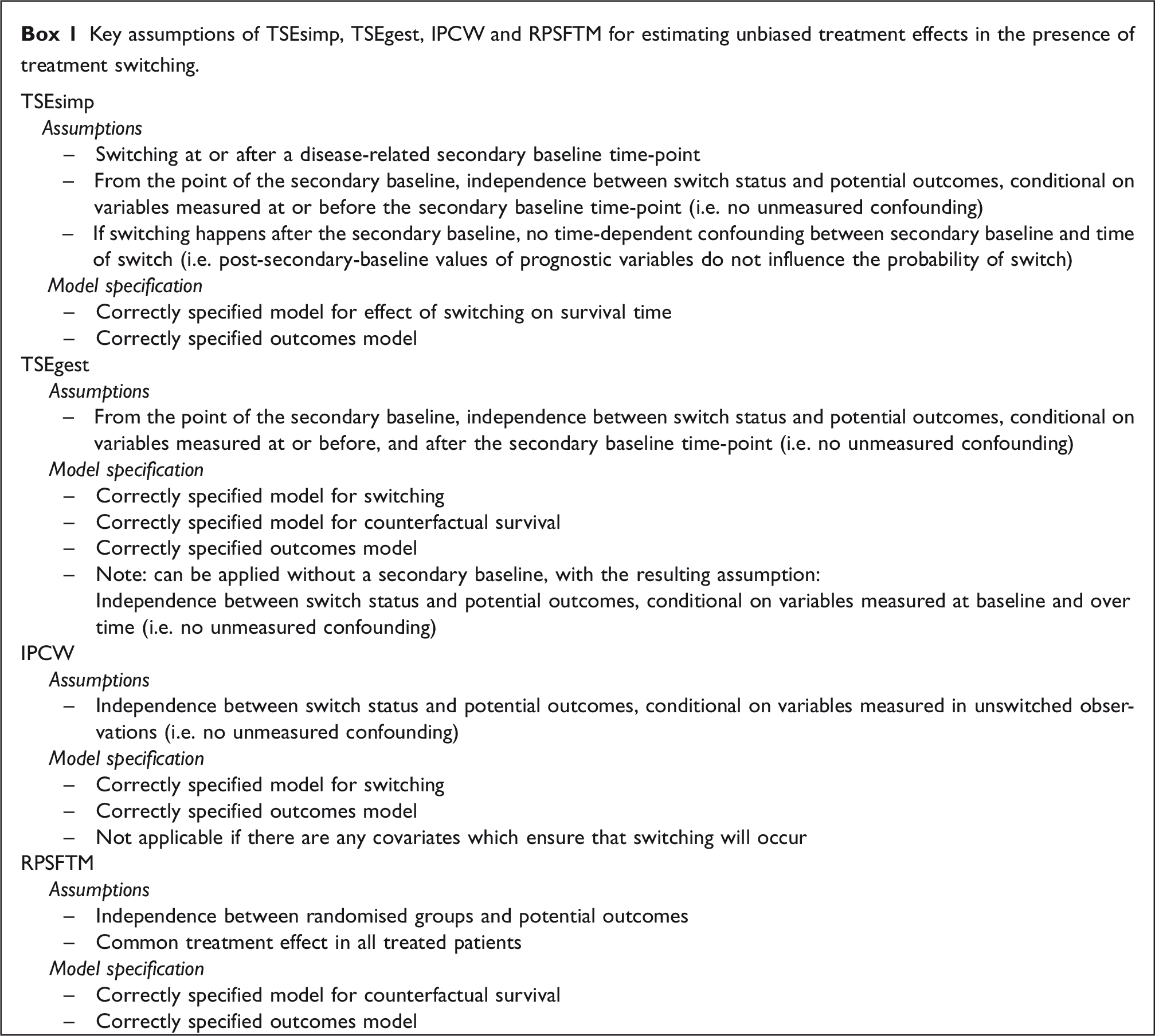

TSEsimpAssumptions – Switching at or after a disease-related secondary baseline time-point – From the point of the secondary baseline, independence between switch status and potential outcomes, conditional on variables measured at or before the secondary baseline time-point (i.e. no unmeasured confounding) – If switching happens after the secondary baseline, no time-dependent confounding between secondary baseline and time of switch (i.e. post-secondary-baseline values of prognostic variables do not influence the probability of switch)Model specification – Correctly specified model for effect of switching on survival time – Correctly specified outcomes model

TSEgestAssumptions – From the point of the secondary baseline, independence between switch status and potential outcomes, conditional on variables measured at or before, and after the secondary baseline time-point (i.e. no unmeasured confounding)Model specification – Correctly specified model for switching – Correctly specified model for counterfactual survival – Correctly specified outcomes model – Note: can be applied without a secondary baseline, with the resulting assumption:Independence between switch status and potential outcomes, conditional on variables measured at baseline and over time (i.e. no unmeasured confounding)

IPCWAssumptions – Independence between switch status and potential outcomes, conditional on variables measured in unswitched observations (i.e. no unmeasured confounding)Model specification – Correctly specified model for switching – Correctly specified outcomes model – Not applicable if there are any covariates which ensure that switching will occur

RPSFTMAssumptions – Independence between randomised groups and potential outcomes – Common treatment effect in all treated patientsModel specification – Correctly specified model for counterfactual survival – Correctly specified outcomes model

2.1.1 Two-stage estimation – simple approach

2.1.1.1 TSEsimp – concept

As previously described, TSE is designed to adjust for switching that occurs after a specific disease-related time-point, referred to as a “secondary baseline”.¹² The TSE method involves first estimating the effect associated with switching treatments and then using this estimated effect to derive counterfactual survival times for switchers – those that would have been observed if switching had not occurred.

2.1.1.2 TSEsimp – assumptions

The simple TSE approach, TSEsimp, relies on three assumptions (see Box 1):¹² (i) Switching must only occur at or after a disease-related secondary baseline time-point; (ii) from the point of the secondary baseline, switching is independent of potential outcomes, conditional on variables measured at or before the secondary baseline time-point, and; (iii) if switching happens after the secondary baseline, there must be no time-dependent confounding between the secondary baseline time-point and the time of switch – that is, post-secondary baseline values of prognostic variables must not influence the probability of switching. Essentially, there must be no confounding that is not accounted for in the TSEsimp model used to estimate the effect of switching. This is referred to as no unmeasured confounding, where a confounder is a variable that influences the treatment decision and is prognostic for the outcome of interest (i.e. survival).

2.1.1.3 TSEsimp – modelling approach

TSEsimp involves a model for the effect of treatment switching on survival time and an outcomes model, which may be used to estimate the effect of the intervention on survival using the estimated survival times from the adjustment procedure. These models must be correctly specified in order for TSEsimp to provide appropriate estimates of the effect of being randomised to experimental treatment adjusted for treatment switching (see Box 1).

A standard parametric accelerated failure time model (e.g. Weibull or Generalised Gamma) is used to estimate the effect of switching on survival time.¹² Post-secondary-baseline survival times in control group switchers are compared to those in control group non-switchers. The model includes covariates for prognostic characteristics measured at the secondary baseline time-point or before in an attempt to account for potential prognostic differences between switchers and non-switchers, and a switching variable which equals ‘1’ after the time of switch. The model provides an estimate of the treatment effect associated with switching in the form of a time-ratio, representing a multiplicative factor by which an individual’s expected survival time is increased (or decreased) by being on the treatment switched to, referred to as $e^{- ψ}$ .

The inverse of the treatment effect, i.e. $e^{ψ}$ , is then used to estimate counterfactual survival times ( $U_{i}$ ) for switchers. This implies using the causal interpretation of the model used to estimate the effect of treatment switching on survival times. The model assumes that treatment has a multiplicative effect on survival time and splits the observed event time, $T_{i}$ , for each patient into time spent on the control treatment, $T_{C i}$ , and time spent on the experimental treatment, $T_{E i}$ . For control group switchers, $T_{C i}$ is equal to the time from randomisation until switching occurs, and $T_{E i}$ is equal to the time from switch until death or censoring. For non-switchers in the control group, $T_{E i} = 0 .$ The structural model for counterfactual survival times is therefore specified as follows:

U_{i} = T_{C i} + e^{ψ} T_{E i}

(1)

Using equation (1), survival times are estimated for switching patients under a counterfactual scenario where they did not switch. For each switcher, values for $T_{C}$ and $T_{E}$ are plugged into equation (1), along with the estimate of $e^{ψ}$ taken from the parametric accelerated failure time model used to estimate the effect of switching on survival time. Thereby, counterfactual survival times are estimated for switchers. In the absence of censoring, the adjustment for treatment switching is complete. However, if censoring is present, an additional step called “re-censoring” is required.^23–25 For switchers who are not observed to die, the model for counterfactual survival times results in a shrunken censoring time (assuming the treatment is beneficial). If switching is related to prognostic factors, shrinking censoring times in switchers (and not in non-switchers) will result in informative censoring because censoring times will be related to prognosis. Re-censoring breaks the dependence between the counterfactual censoring time and treatment received.^23–25 The counterfactual survival time associated with a given value of $ψ$ (that is, $U_{i} (ψ)$ ) is re-censored for all patients in the treatment group in which switching occurs at the minimum of the administrative censoring time $C_{i}$ and $e^{ψ} C_{i}$ , representing the earliest possible censoring time over all possible treatment trajectories, $D_{i}^{*} (ψ)$ . $U_{i} (ψ)$ is then replaced by $D_{i}^{*} (ψ)$ if $D_{i}^{*} (ψ) < U_{i} (ψ)$ . Re-censoring results in a loss of longer term information, which can be problematic if the aim is to estimate long-term treatment effects – this is discussed elsewhere.²⁶

After estimating untreated survival times for switchers and undertaking re-censoring if required, a new dataset is derived consisting of a mixture of observed (for non-switchers) and adjusted (for switchers) survival times. This dataset may be used to compare experimental and control group survival times using any outcomes model, to estimate the effect of experimental treatment adjusted for treatment switching. For instance, a Cox proportional hazards model might be used to estimate a hazard ratio.²⁷ Confidence intervals produced by the outcomes model will be inappropriate because they do not take into account that survival times have been adjusted in switchers – bootstrapping the entire adjustment process is recommended to appropriately characterise uncertainty.^1,12

2.1.1.4 TSEsimp – a variation

TSEsimp relies upon simple regression and does not attempt to adjust for time-dependent confounders. A variation of this approach is to include time-dependent variables in the simple regression model used to estimate the effect of switching. For reasons previously described and illustrated in Figure 4, this approach is prone to bias. However, in order to highlight the inadequacies of using simple regression adjustment to control for time-dependent confounding, we include this approach in this study, denoted TSEsimpTDC.

2.1.2 Two-stage Estimation – g-estimation approach

2.1.2.1 TSEgest – concept

Through its use of g-estimation and a structural nested model (SNM), TSEgest allows the assumptions of TSEsimp to be relaxed because it is capable of dealing with time-dependent confounding, provided its own assumptions hold.^20,28,29 Importantly, the method does not even require that a secondary baseline exists – for instance, it is applicable if switching happens before or after disease progression. However, in this study we are interested in a situation where switching only happens at or beyond disease progression. In this context, where the risk of switching is zero before progression, it is reasonable to apply TSEgest using disease progression as a secondary baseline. We describe TSEgest in this setting, in which it involves the same concept as TSEsimp – a treatment effect associated with treatment switching is estimated which is then used in a counterfactual survival model to estimate untreated survival times for switchers.

2.1.2.2 TSEgest – assumptions

TSEgest involves modelling switching and relies on one key assumption (see Box 1):²⁹ switching is independent of potential outcomes, conditional on measured variables – that is, there is no unmeasured confounding. It is not a problem if post-secondary-baseline values of prognostic variables influence the probability of switch, provided those variables are measured and included in the analysis.

2.1.2.3 TSEgest – modelling approach

TSEgest involves a model for switching, a counterfactual survival model, and an outcomes model. Each of these models must be correctly specified in order for TSEgest to provide appropriate estimates of the effect of being randomised to experimental treatment adjusted for treatment switching (see Box 1).

The switching model is used in combination with g-estimation to estimate $e^{- ψ}$ , that is, the treatment effect associated with switching in the form of a time-ratio also used by TSEsimp. The no unmeasured confounding assumption means that switching at each measurement occasion is independent of counterfactual survival times $U_{i}$ , conditional on measured variables.²⁰ The switching model therefore relates treatment at each measurement observation to counterfactual survival time given a specific value for ψ, controlling for all confounders and the g-estimation procedure searches for the value of ψ that results in independence between switch status and $U_{i}$ . For instance, from Sterne and Tilling²⁰

logit (p (E_{i k})) = α U_{i, ψ} + \sum_{j} β_{j} x_{ijk}

(2)

where

E_{i k}

is observed switch status for individual i at observation k,

U_{i, ψ}

is the counterfactual survival time for individual i given a specific value for ψ, and

x_{ijk}

are all confounders for individual i at observation k. If TSEgest is applied from a secondary baseline,

U_{i, ψ}

refers to post-secondary-baseline counterfactual survival; the structure of the counterfactual survival model used to estimate this is the same as in (1), but

T_{C i}

refers to the time spent after the secondary baseline on control treatment, and

T_{E i}

refers to the time spent after the secondary baseline on the experimental treatment. The switching model and the post-secondary-baseline counterfactual survival model are used simultaneously to provide the g-estimate of

e^{- ψ}

The g-estimation procedure involves fitting a series of models defined by (2) for a range of values of ψ, searching for the value of ψ (the “g-estimate”) for which switch status at each measurement occasion is independent of $U_{i}$ . This assessment is based on a test statistic for α in equation (2) that is zero (that is, the P-value is 1), meaning that there is no association between current treatment and $U_{i, ψ}$ . Typically a Wald statistic is used.²⁰ The upper and lower limits of the 95% confidence interval for ψ are the two values for which the two-sided P-values for the test statistic of α are 0.05.

Once ψ has been identified, it is used in equation (1) to estimate counterfactual survival times for patients who switched treatments, as in TSEsimp, resulting in a new dataset consisting of a mixture of observed and unobserved survival times. When censoring is present, re-censoring is required. Then, an outcomes model is used to estimate the effect of experimental treatment adjusted for treatment switching. Again, bootstrapping of the entire adjustment process is required to appropriately characterise uncertainty.

2.1.3 Inverse probability of censoring weights

2.1.3.1 IPCW – concept

IPCW can be used to adjust for treatment switching and can cope with time-dependent confounders. IPCW involves censoring patients at the time of switch but then weighting remaining observations using information on baseline and time-dependent patient characteristics to avoid the selection bias associated with the censoring.^1,18

2.1.3.2 IPCW – assumptions

IPCW involves modelling the switching process and is reliant on one key assumption (see Box 1): that there is no unmeasured confounding.^1,18,29 The definition of a confounder is the same as for the TSE methods – that is, a variable that influences the probability of switching and is prognostic for survival. Therefore, data must be available on all such variables.^30,31

2.1.3.3 IPCW – modelling approach

IPCW involves a switching model and an outcomes model. The switching model is used to estimate weights, which are then used in the outcomes model to estimate a treatment effect adjusted for treatment switching. These models must both be correctly specified in order for IPCW to provide unbiased estimates of the effect of being randomised to experimental treatment, adjusted for treatment switching (see Box 1). The method is not applicable if there are any covariate patterns which ensure (i.e. the probability equals 1) that treatment switching will occur.^18,31,32

IPCW is often applied working in discrete time, dividing follow-up into small intervals and using pooled logistic regression.¹⁸ First, a model for switching is fitted, controlling for all baseline and time-varying confounders. This model is used to estimate the probability of switching for each individual in each interval. An individual’s probabilities of remaining unswitched up to interval t are then multiplied together, with the weight representing the inverse probability of remaining unswitched up to interval t. These weights can be highly variable, decreasing statistical efficiency,³³ and therefore stabilised weights are often used instead¹⁸

\hat{W} (t) = \prod_{k = 0}^{t} \frac{\hat{\Pr} [C (k) = 0 | \bar{C} (k - 1) = 0, \bar{A} (k - 1), V, T > k]}{\hat{\Pr} [C (k) = 0 | \bar{C} (k - 1) = 0, \bar{A} (k - 1), \bar{L} (k), T > k]}

(3)

where

C (k)

is an indicator function demonstrating whether or not switching had occurred at the end of interval

k

, and

\bar{C} (k - 1)

denotes switching history to the end of the previous interval.

\bar{A} (k - 1)

denotes an individual’s treatment history up to the end of the previous interval, and

V

is an array of an individual’s baseline covariates.

\bar{L} (k)

denotes the history of an individual’s time-dependent covariates measured at or prior to the beginning of interval

k

and includes

V

. Only baseline and time-dependent confounding variables need to be included in

V

and

\bar{L} (k)

The denominator of equation (3) represents the probability of an individual remaining unswitched at the end of interval k given that he or she had not switched at the end of the previous interval $(k - 1)$ , conditional on baseline confounders, time-dependent confounders and treatment history – as estimated by the switching model. The numerator of equation (3) represents that same probability, but is conditional only on baseline confounders and treatment history. For unstabilised weights, this numerator would simply equal 1. The idea behind stabilised weights is that the numerator is made as similar as possible to the denominator without re-introducing confounding – time-dependent confounders must not be included in the numerator.³⁴

Inverse probability weights can be incorporated within any outcomes model to adjust for treatment switching. Any baseline confounders $V$ included in the numerator of the weighting model should be included in the weighted outcomes model.¹⁷ Ordinary standard errors are not valid in a weighted analysis and these must instead be computed in a robust way, using the sandwich variance.

2.1.4 Rank preserving structural failure time models

2.1.4.1 RPSFTM – concept

The RPSFTM involves a similar concept to TSEsimp and TSEgest – a treatment effect associated with switching is estimated and this is used to derive what survival times would have been in the absence of switching. Unlike the TSE methods, the RPSFTM does not differentiate between the treatment effect in the experimental group and the treatment effect in switchers – the treatment effect $e^{- ψ}$ is assumed to be the same irrespective of when treatment is received. This may be regarded as a disadvantage, particularly in the context of post-progression switching in an oncology trial, as progressive disease may alter capacity to benefit. However, by making this assumption – in combination with g-estimation designed specifically for an RCT context – the RPSFTM avoids the no unmeasured confounding assumption.^16,35

2.1.4.2 RPSFTM – assumptions

The RPSFTM makes two crucial assumptions (see Box 1): (i) Potential outcomes are independent of randomised group, and (ii) there is a common treatment effect (that is, the time ratio ψ is equal for all treated patients).^16,35

2.1.4.3 RPSFTM – modelling approach

The RPSFTM involves a counterfactual survival model to estimate untreated survival times for all randomised patients, and an outcomes model used to estimate the effect of experimental treatment adjusted for treatment switching. These models must be correctly specified in order for RPSFTM to provide unbiased estimates of the effect of being randomised to experimental treatment adjusted for treatment switching (see Box 1).

For the simple one-parameter RPSFTM, the counterfactual survival model splits the observed event time ( $T_{i}$ ) for each patient into the time spent on the control treatment ( $T_{C i}$ ) and the time spent on the experimental treatment ( $T_{E i}$ ). $T_{i}$ is related to the counterfactual event time ( $U_{i}$ ) with the same model as presented in equation (1). The value of ψ is estimated using g-estimation.²⁸ For a range of values of ψ, the counterfactual survival model (1) is used to estimate $U_{i}$ , and the true value is that which results in $U_{i}$ being independent of randomised groups, based upon a g-test.³⁶ The g-test (e.g. log-rank, Cox) tests the hypothesis that the counterfactual (untreated) survival curves are identical in the two treatment groups, with the point estimate of ψ being that for which the test (z) statistic equals zero.

The g-estimation process results in counterfactual survival times estimated for the g-estimate of ψ. A new dataset is derived consisting of observed survival times for experimental group patients and control group non-switchers, and counterfactual survival times for switchers. When censoring is present, re-censoring (for all patients in treatment groups affected by switching) is incorporated within the g-estimation process. Then, an outcomes model is used to estimate the effect of experimental treatment adjusted for treatment switching. The P-value produced by the outcomes model is likely to be too small and confidence intervals too narrow because they do not account for the fact that the data have been adjusted. It is recommended that the P-value from an equivalent ITT analysis should be used and confidence intervals calculated accordingly^16,37 or, as for the TSE methods, the entire adjustment procedure could be bootstrapped.

2.2 Simulation study

Detailed information on our simulation study, including code used to simulate the data, is provided in the appendices. Here we provide a brief summary of our aims, data generating mechanism, estimand, methods included and performance measures. The simulation study was conducted using Stata software, version 14.2.³⁸

2.2.1 Aims

Our objective was to assess the performance of TSEgest compared to TSEsimp, IPCW and RPSFTM in adjusting for treatment switching in simple scenarios, where time-dependent confounding is not an issue, and in more complex scenarios affected by time-dependent confounding. We focus on the problem typically seen in HTA whereby a subset of patients randomised to the control group of an RCT switch onto the experimental treatment after disease progression. Our aim is to estimate what survival would have been in the control group if switching had not occurred.

2.2.2 Data generating mechanism

In common with previous simulation studies,^13,26 we simulated datasets with a sample size of 500 and 2:1 randomisation in favour of the experimental group, and with treatment switching permitted from the control group onto the experimental treatment. A step-by-step description of our data generating mechanism is provided in online Appendix A.

Our primary interest was in the performance of the adjustment methods in scenarios when time-dependent confounding was present, and when time-dependent confounding was not present. To this end, we simulated a set of ‘simple’ scenarios (which did not include time-dependent confounding) and a set of ‘complex’ scenarios (where time-dependent confounding was present). In the ‘simple’ scenarios, control group patients could only switch onto the experimental treatment immediately upon disease progression – no switching before or after this time point was allowed. Hence, there could be no time-dependent confounding between the time of progression and the time of switch. In the ‘complex’ scenarios, control group patients could switch onto the experimental treatment either immediately upon disease progression or beyond this time point. A post-progression confounding variable (referred to as ‘metastatic disease’) was simulated to ensure that these scenarios were affected by time-dependent confounding. In addition, there was an interaction between the effect of switching and the metastatic disease variable. In patients who had not yet developed metastatic disease, switching treatments reduced the probability of subsequently developing metastatic disease. In patients who had developed metastatic disease, switching treatments extended survival but did not alter the fact that metastatic disease had been developed. Hence treatment effect heterogeneity was present.

In addition to the existence of time-dependent confounding, we considered that the size of the treatment effect, the switching proportion, and whether or not censoring was present could affect the performance of the adjustment methods. Hence, scenarios were run varying the following characteristics:

Treatment effect: low (average HR under the assumption of proportional hazards (which is an incorrect assumption in complex scenarios) approximately 0.82); high (average HR approximately 0.61)

Switch proportion: moderate (approximately 50% of control group patients who experienced disease progression); high (approximately 75% of control group patients who experienced disease progression)

Censoring: none; present (administrative censoring proportion approximately 20–35%)

Time-dependent confounding: none (in simple scenarios); present (in complex scenarios)

Using a 2 × 2×2 × 2 factorial design resulted in a total of 16 scenarios. The scenarios were numbered 1–16 with all levels of one factor nested inside one level of the next factor, following the order listed above. Details on scenario values and settings are presented in online Appendices B and C. Scenarios 1–8 were the simple scenarios, in which the metastatic disease time-dependent confounder was not included. Scenarios 9–16 were the complex scenarios, which included the time-dependent confounder. Scenarios 15 and 16 were re-run simulating a sample size of 10,000 instead of 500, because we anticipated that IPCW and TSEgest may be prone to high error levels with relatively small sample sizes. Repeating these scenarios with a much larger sample size allowed us to assess this. Therefore, in total 18 scenarios were run. One thousand simulations were run for each scenario.

2.2.3 Estimand

Our estimand was restricted mean survival time (RMST) in the control group, consistent with our aim of investigating the performance of adjustment methods in estimating survival times for the control group that would have been observed in the absence of treatment switching.

In the simple scenarios, it was possible to integrate the simulated survival function to calculate true RMST (see equations (A1) to (A3) in online Appendix A). In the complex scenarios, the survival function was not analytically tractable, so to estimate our “true” value for each scenario, we simulated data for 1,000,000 patients without incorporating treatment switching, and estimated control group RMST by calculating the area under the Kaplan–Meier survival function. This value is the product of a simulation so is prone to error, but this is minimal given the large number of patients simulated. For instance, in Scenario 1, the standard error of the control group RMST estimate of 424.37 days was 0.48. In scenarios that did not include censoring, RMST was effectively unrestricted because death was observed in all simulated patients. In scenarios that included censoring, RMST was estimated up to 546 days (the maximum administrative censoring time in the simulated datasets).

2.2.4 Adjustment methods compared

TSEsimp, TSEgest, RPSFTM and IPCW were included and their application is described in detail in online Appendix D. TSEsimpTDC was only included in Scenarios 9–18 because in Scenarios 1–8, where switching could only occur immediately at the point of disease progression, TSEsimpTDC simplifies to TSEsimp. As described previously, TSEsimp (and TSEsimpTDC), TSEgest and RPSFTM involve estimating a treatment effect associated with switching and then using this to derive counterfactual survival times, whereas IPCW results in weighted survival times. We used the Stata command stpm2³⁹ to fit flexible parametric models to the counterfactual datasets provided by TSEsimp, TSEsimpTDC, TSEgest and RPSFTM, and to the weighted survival times provided by IPCW, to obtain the survivor function extrapolated (if necessary) to 546 days, ensuring that our RMST comparisons were comparing “like with like”. Non-parametric methods to estimate RMST up to the final follow-up time-point could not be used because, in scenarios that included censoring, when re-censoring is applied (for the TSE and RPSFTM methods) the re-censored final follow-up time-point may differ from 546 days and may differ for each adjustment method. Using flexible parametric models is consistent with UK HTA recommendations for undertaking survival modelling in the presence of complex hazard functions.^40,41

To provide context on the performance of the various adjustment methods, we included a ‘No Switching’ analysis, representing the results of a standard ITT analysis (that is, an unadjusted estimate of control group RMST) undertaken on the simulated dataset before switching was applied. This represents the “truth” for each simulation and does not represent a feasible estimator, but provides a useful upper bound for adjustment method performance which may be considered a ‘gold standard’. We also included a standard ITT analysis after switching was applied. Though this has a different estimand to the adjustment methods (because it does not adjust for switching), it is standard practice to present an ITT analysis even in the presence of treatment switching.

2.2.5 Performance measures

The performance of methods was evaluated according to the percentage bias in their estimate of control group RMST at 546 days. Percentage bias was estimated by taking the difference between the mean estimated RMST and the true RMST and expressing this as a percentage of true RMST.⁴² Root mean squared error (RMSE) and empirical standard errors (SE) of the RMST estimates were also calculated for each method and expressed as percentages of the true RMST. Convergence was measured, defined as the proportion of times that each method resulted in an estimate of control group RMST. Percentage bias, RMSE and empirical SE were calculated based upon simulations in which convergence occurred. Monte Carlo (MC) standard errors were calculated for each performance measure, for each method.⁴³ For the IPCW method, we recorded the mean, standard deviation, minimum, maximum and coefficient of variation of the weights measured across control group patients in each simulated data set, in order to explore the relationship between these and the performance of the method.

3 Results

First, we present results from the simple scenarios, focusing on results from one scenario to illustrate the key findings. We then repeat this for the complex scenarios. A summary table describing the data generated under each scenario is presented in online Appendix E.

3.1 Results from simple scenarios

The upper half of Table 1 presents detailed results from Scenario 2, which included no time-dependent confounder, a large treatment effect, a moderate switch proportion and zero censoring. The ITT analysis over-estimated control group RMST, equivalent to a percentage bias of 12.4%. TSEsimp, TSEgest, RPSFTM and IPCW all predicted control group RMST with very little percentage bias, ranging from 0.0% for RPSFTM to 1.0% for TSEgest. TSEsimp resulted in empirical standard errors and RMSE that were approximately 10–13% lower than those from TSEgest, RPSFTM and IPCW.

Table 1.

Scenarios 2 and 10 – performance measures for estimation of control arm RMST.

Scenario details	Method	Percent bias in RMST	Empirical SEas percentage of true RMST	RMSEas percentage of true RMST	Convergence (%)
Scenario number: 2True RMST:Control: 424Experimental: 600Mean switch: 50%True ave. HR: 0.61True ave. TR: 1.42Mean censored: 0%	No switching	−0.0	5.5	5.5	100
	ITT	12.4	6.3	13.9	100
	TSEsimp	0.4	7.4	7.4	100
	TSEgest	1.0	8.2	8.3	100
	RPSFTM	0.0	8.2	8.2	100
	IPCW	0.6	8.1	8.1	100
	min/max MC error	0.2/0.3	0.1/0.2	0.1/0.2	–
Scenario number: 10True RMST:Control: 338Experimental: 465Mean switch: 51%True ave. HR: 0.65True ave. TR: 1.38Mean censored: 0%	No switching	−0.1	5.5	5.5	100
	ITT	7.3	6.0	9.5	100
	TSEsimp	5.6	7.0	9.0	100
	TSEsimpTDC	6.9	7.4	10.1	100
	TSEgest	−0.6	6.4	6.4	100
	RPSFTM	−0.1	7.0	7.0	100
	IPCW	0.6	7.0	7.0	100
	min/max MC error	0.2/0.2	0.1/0.2	0.1/0.2	–

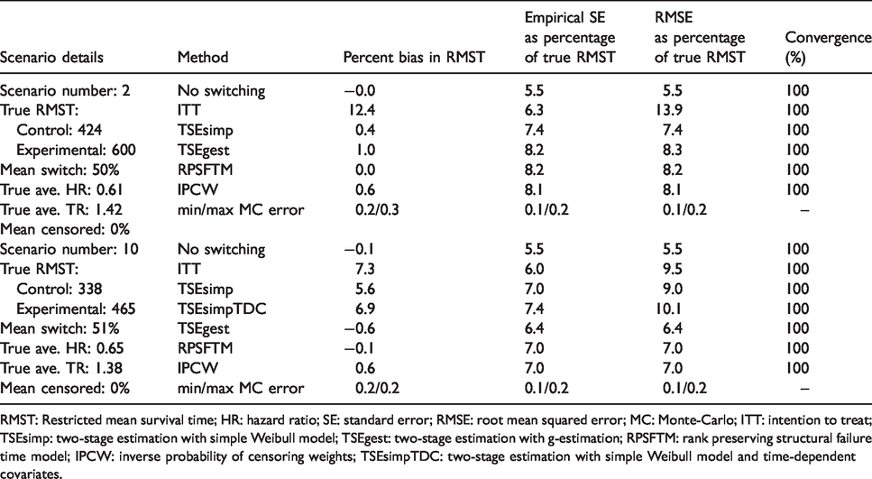
RMST: Restricted mean survival time; HR: hazard ratio; SE: standard error; RMSE: root mean squared error; MC: Monte-Carlo; ITT: intention to treat; TSEsimp: two-stage estimation with simple Weibull model; TSEgest: two-stage estimation with g-estimation; RPSFTM: rank preserving structural failure time model; IPCW: inverse probability of censoring weights; TSEsimpTDC: two-stage estimation with simple Weibull model and time-dependent covariates.

Results were similar across all simple scenarios (Scenarios 1–8) for all methods except IPCW and ITT, as illustrated by Figures 5 to 7, which present nested loop plots for percentage bias, empirical SE and RMSE across all scenarios.⁴⁴ Across Scenarios 1–8, TSEsimp and IPCW resulted in least percentage bias in three scenarios apiece and RPSFTM resulted in least percentage bias in two scenarios. All methods always had percentage bias of less than 1.4%, except IPCW which resulted in percentage bias of approximately 3% in Scenarios 3 and 4, in which the switching proportion was high. TSEsimp consistently generated lower empirical standard errors than the other adjustment methods in the simple scenarios, with these ranging between 0% and 20% lower than the empirical standard errors associated with TSEgest, 11–49% lower than those associated with RPSFTM, and 9–63% lower than those associated with IPCW. This contributed to TSEsimp always resulting in the lowest RMSE of all the adjustment methods in the simple scenarios.

Figure 5.

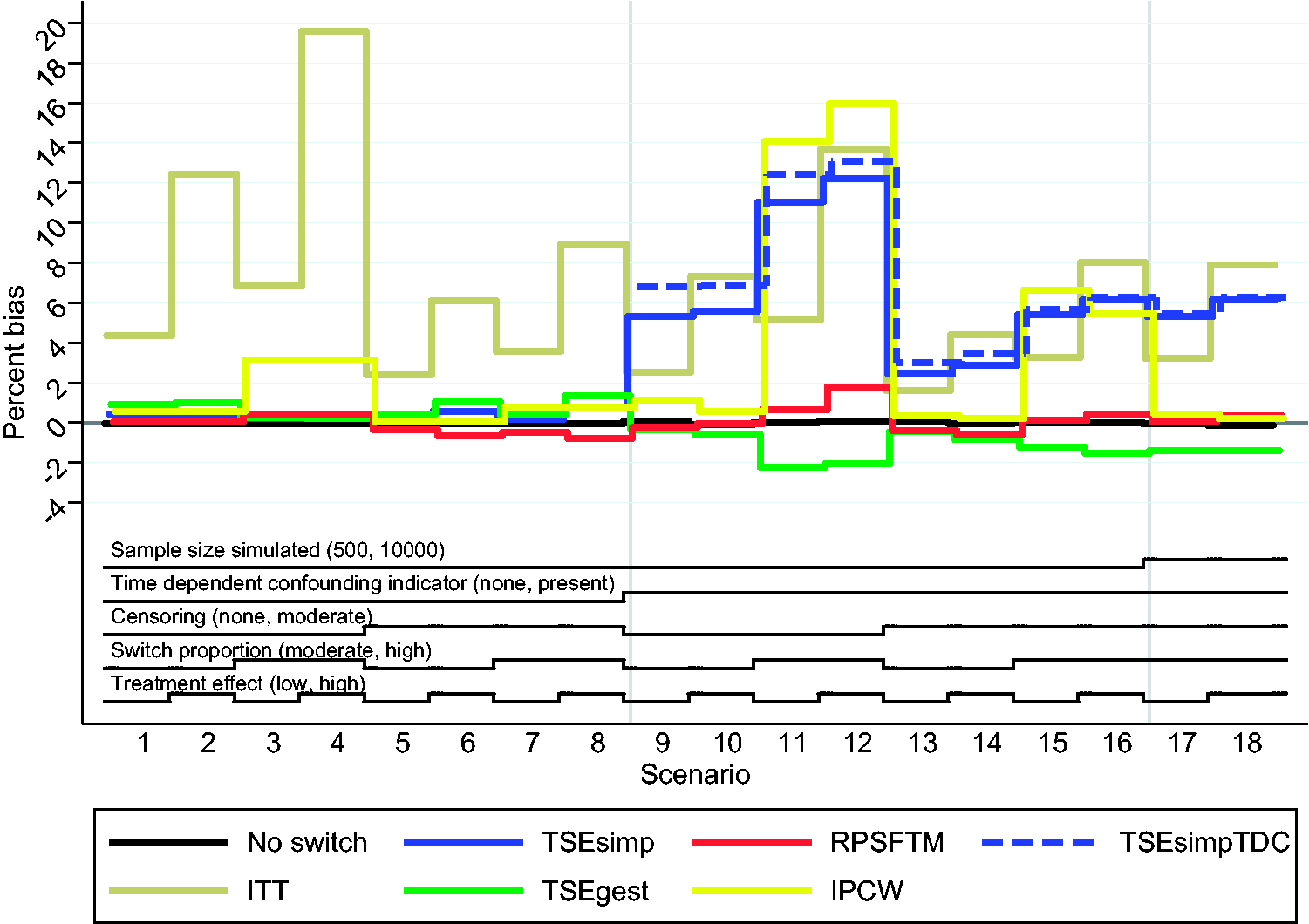
Percentage bias in estimation of control group restricted mean survival time across all scenarios. ITT: intention to treat; TSEsimp: two-stage estimation with simple Weibull model; TSEgest: two-stage estimation with g-estimation; RPSFTM: rank preserving structural failure time model; IPCW: inverse probability of censoring weights; TSEsimpTDC: two-stage estimation with simple Weibull model and time-dependent covariates.

Figure 6.

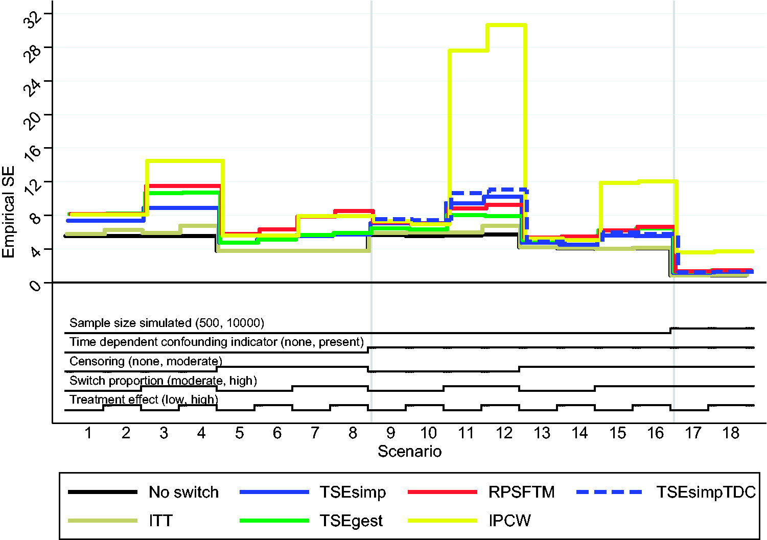
Empirical standard error in estimation of control group restricted mean survival time across all scenarios. ITT: intention to treat; TSEsimp: two-stage estimation with simple Weibull model; TSEgest: two-stage estimation with g-estimation; RPSFTM: rank preserving structural failure time model; IPCW: inverse probability of censoring weights; TSEsimpTDC: two-stage estimation with simple Weibull model and time-dependent covariates; SE: standard error.

Figure 7.

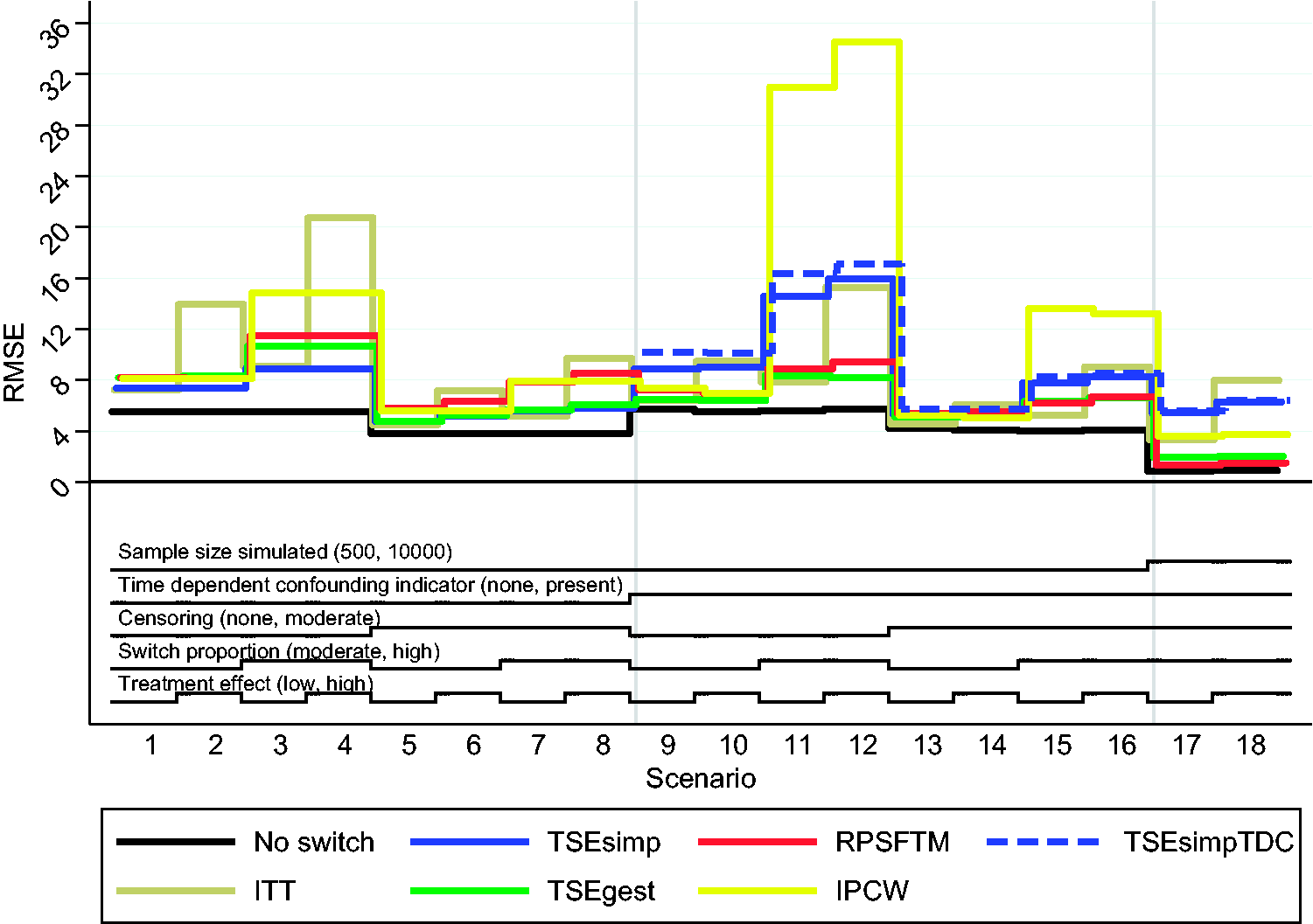
Root mean squared error in estimation of control group restricted mean survival time across all scenarios. ITT: intention to treat; TSEsimp: two-stage estimation with simple Weibull model; TSEgest: two-stage estimation with g-estimation; RPSFTM: rank preserving structural failure time model; IPCW: inverse probability of censoring weights; TSEsimpTDC: two-stage estimation with simple Weibull model and time-dependent covariates; RMSE: root mean squared error.

3.2 Results from complex scenarios

Table 1 also presents detailed results from Scenario 10, which was similar to Scenario 2 with respect to treatment effect, switch proportion and censoring, but included time-dependent confounding. The ITT analysis again over-estimated control group RMST, equivalent to a percentage bias of 7.3%. TSEsimp resulted in high percentage bias in Scenario 10 – over-estimating control group RMST to almost the same extent as the ITT analysis (percentage bias 5.6%). In contrast, TSEgest, RPSFTM and IPCW generated very low percentage bias (−0.6% for TSEgest, −0.1% for RPSFTM and 0.6% for IPCW). TSEsimpTDC resulted in percentage bias (6.9%) that was similar in size to that of TSEsimp. TSEgest resulted in an empirical standard error that was approximately 10% lower than that of TSEsimp, RPSFTM and IPCW, and also generated the lowest RMSE. TSEsimp produced substantially higher RMSE due to its increased bias.

Results for RPSFTM and TSEgest were relatively stable in all the complex scenarios, as illustrated in Figures 5 to 7. These methods consistently resulted in low bias, although TSEgest was prone to slightly increased bias (up to approximately 2%) in scenarios with a high switching proportion. TSEsimp (and TSEsimpTDC) consistently resulted in much higher levels of bias than TSEgest and RPSFTM, with increased switching proportions and treatment effect sizes associated with higher bias. IPCW resulted in low bias in Scenarios 9, 10, 13 and 14, when the switching proportion was moderate (approximately 50%), but produced much higher bias in Scenarios 11, 12, 15 and 16, when the switching proportion was high (approximately 75%).

The switching proportions in Scenarios 11–12 and 15–16 were not different to those simulated in simple Scenarios 3–4 and 7–8, in which IPCW resulted in low bias. However, the incorporation of the time-dependent confounding variable meant that additional covariates were used in the TSEgest and IPCW switching models, which, combined with a low sample size and high switching proportion resulted in slightly increased bias for TSEgest and substantially increased bias for IPCW. Re-running Scenarios 15 and 16 with a much larger sample size (in Scenarios 17 and 18) had minimal impact on TSEgest, but resulted in substantially reduced bias for IPCW. In Scenarios 17 and 18, IPCW produced weights that were much lower as a proportion of the size of the group being subjected to weighting, compared to Scenarios 15 and 16 (and Scenarios 11 and 12). Within Scenarios 1–16, the range of weights was widest in Scenarios 11, 12, 15 and 16, with average minimum and maximum weights of approximately 0.02 and 18 in these scenarios, in a control group made up of approximately 170 patients. The coefficient of variation of the weights was also highest in these scenarios (approximately 0.77) but this was not substantially different to the coefficient of variation in scenarios in which the IPCW worked well (e.g. Scenarios 3, 4, 7 and 8). In Scenarios 17 and 18, the range of weights and the coefficient of variation increased (average minimum and maximum weight 0.02 and 71, coefficient of variation 0.98–0.99), but the maximum weight was much lower as a proportion of the size of the group being subjected to weighting, as approximately 3400 patients were randomised to the control group in these scenarios. This indicates that it is the size of the maximum weight in relation to the size of the group being subjected to weighting that is a key determinant of the bias associated with IPCW. In Scenarios 1–8, the maximum weight as a proportion of the control group sample size varied between 3% and 6% and in Scenarios 9–10, 13–14 and 17–18 it was approximately 2%. However, in Scenarios 11, 12, 15 and 16, this proportion increased to 10–11%.

Across Scenarios 9–18, RPSFTM generated least percentage bias in seven scenarios and IPCW in three scenarios. Neither TSEsimp or TSEgest resulted in least percentage bias in any of these scenarios, but percentage bias was considerably lower for TSEgest than TSEsimp in all of these scenarios, and levels of bias associated with TSEgest were not substantially different from those associated with RPSFTM. IPCW resulted in much higher percentage bias than TSEgest and RPSFTM in Scenarios 11, 12, 15 and 16. TSEsimp produced lower empirical standard errors than the other adjustment methods in scenarios which incorporated censoring (Scenarios 13–18), but TSEgest produced the lowest empirical standard errors in scenarios without censoring (Scenarios 9–12). Across Scenarios 9–18, TSEgest resulted in lowest RMSE in six scenarios, RPSFTM in three scenarios and IPCW in one scenario.

4 Discussion

In scenarios without time-dependent confounding, TSEsimp resulted in estimates of control group RMST that had similar or lower bias than the complex adjustment methods, and had less variability. However, in scenarios with time-dependent confounding, TSEsimp resulted in estimates that had substantially higher bias than TSEgest and RPSFTM. IPCW also resulted in substantially lower bias than TSEsimp in scenarios with time-dependent confounding, provided the inverse probability weights were not too high. Overall, if time-dependent confounding is unlikely, TSEsimp remains an appropriate adjustment method. But if time-dependent confounding is a possibility – for instance, due to long time periods between the secondary baseline and the switching time, or due to measured prognostic events that occurred between these two time-points – TSEgest, RPSFTM and IPCW should be considered instead.

In scenarios with time-dependent confounding, TSEsimp over-estimated control group RMST to almost the same extent as the ITT analysis – sometimes actually resulting in a higher estimate of control group RMST than the ITT analysis. This is because patients who experienced the metastatic event (which drastically reduced survival times) were more likely to switch (as explained in online Appendix A). Failing to account for this constitutes confounding by indication and results in switching appearing to have only a very minor beneficial effect, or in fact in switching appearing harmful. The opposite would be the case if switching was more likely in patients who had not experienced the metastatic event. Either way, in the presence of such time-dependent confounding, TSEsimp becomes prone to high levels of bias. Controlling for a time-dependent confounder using simple regression is inadequate and inappropriate, because we control for a variable through which treatment has an effect on the outcome of interest – as demonstrated by the biased results associated with the TSEsimpTDC analyses.

We demonstrated that correctly specified TSEgest and IPCW models were able to deal with the time-dependent confounding caused by the metastatic disease variable. Interestingly, TSEgest was more robust to high switching proportions in small sample sizes than IPCW. This is in line with theory, because when positivity begins to break down in a particular subgroup (due to very small numbers of patients who do not switch), IPCW is more prone to error because it weights remaining observations in that subgroup – often resulting in very high weights – whereas TSEgest remains able to estimate the treatment effect using data from other subgroups. In practice, violations of the positivity assumption are possible when certain prognostic characteristics are highly predictive for switching. Our IPCW results reflect previous findings, with the added reassurance that the method can perform well even in the presence of serious time-dependent confounding – provided models are accurately specified and weights are not too high. Previous studies have demonstrated that IPCW performs well when weights are not extreme,^12,13,26,45 and have discussed the definition of weights that are too high or have too great a range or coefficient of variation.^12,13,26 In this study we found that the coefficient of variation did not seem to be the most important determinant of bias associated with IPCW – instead it appeared that the size of the weights in relation to the sample size of the group subject to weighting was the critical factor. We are unable to draw firm conclusions, but we found that when the maximum weight as a proportion of the group being weighted was less than 6%, the IPCW method resulted in low bias, but when this proportion increased to 10–11% bias increased substantially.

Our study also provides further information on the performance of the RPSFTM, which performed well across all scenarios, often resulting in the lowest percentage bias in scenarios that involved time-dependent confounding – though TSEgest more often generated the lowest RMSE in these scenarios. It is important to note – and is a limitation of our study – that we only simulated scenarios that involved an approximately common treatment effect between switchers and patients randomised to the experimental group. Previous studies have consistently shown that RPSFTM performs well in these circumstances,^12–14,26 although these have not involved important time-dependent confounding variables similar to the metastatic disease variable simulated in this study. Hence, our results provide increased confidence that the RPSFTM method is reliable even in the presence of serious time-dependent confounding. However, as previously demonstrated,^12,13,26 performance of the RPSFTM worsens when the common treatment effect assumption does not hold and sensitivity analysis should always be undertaken around this.⁶ Linked to this, the RPSFTM method is only likely to be appropriate in situations where treatment switching is between randomised treatments. In contrast, TSE and IPCW methods could be used irrespective of what treatment patients switched on to.

It is useful to note that using g-estimation substantially increases the flexibility of the TSE adjustment method – the approach may be thought of as generalised TSE. In fact, because the approach can account for time-dependent confounding, it is not necessary to use a secondary baseline. If treatment switching was only permitted after disease progression, the SNM could be fit from baseline with disease progression included as a time-dependent indicator variable. In such a case, we would expect the model to provide the same results as if it was fitted only from the disease progression time-point, because switching only occurred after progression and thus the switching model would only use data from the point of disease progression onwards – prior observations would be excluded due to perfectly predicting non-switching. However, whilst TSEsimp is not appropriate in circumstances where some (or all) switching occurs before disease progression, TSEgest could be used – representing an important advantage of this approach. An additional practical point worthy of note is that data must be in discrete time interval format for TSEgest to be applied. If variables were measured in continuous time, we would need to discretise time. However, narrow time intervals could be used and we expect that TSEgest could still work well.

Our study has limitations. We used estimates of control group RMST to assess the performance of the adjustment methods. This may seem unexpected given our focus on comparing TSEsimp and TSEgest – two methods that begin by estimating the treatment effect in switchers. However, we could not use this treatment effect as our estimand because this would not have allowed us to make broader conclusions around the performance of the TSE methods in relation to the other adjustment methods. RPSFTM and IPCW do not estimate a treatment effect specific to switchers, so this could not be used as a comparative measure.

The fact that our study consists of simulations may also be considered to be a limitation. Though we investigated several realistic scenarios, these can never cover all situations that may occur in reality. Because we knew the underlying data generating process, we were able to correctly specify switching models for TSEgest and IPCW. In the real world, careful thought must be given to how variables are linked, as model mis-specification will likely result in bias. This illustrates the importance of paying close attention to model specification; it is not enough to simply identify a method that could work, we must consider how the method should actually be applied. In our study we simulated a metastatic disease variable and assumed that this variable had a lagged effect on treatment choices. We think this is realistic – there is often a lag between ordering laboratory tests or scans, receiving the results and making treatment decisions. Therefore, using lagged values of variables in switching models is often likely to be sensible. Careful thought regarding causal pathways is necessary when specifying models that rely on no unmeasured confounding to account for time-dependent confounding, and clinical expert knowledge is likely to be crucial.

It is a limitation that we did not consider coverage in this study. Previous simulation studies have reported coverage, but in a limited way.^12–14,26 To properly account for uncertainty around survival estimates provided by RPSFTM and TSE methods bootstrapping is required, but is not feasible in simulation studies that investigate many scenarios. Without bootstrapping, estimates of coverage are not useful, and so we decided not to include them in this study. In practice, the entire RPSFTM, TSE and IPCW adjustment processes should be bootstrapped to obtain appropriate confidence intervals. In one previous study it was demonstrated that this results in adequate coverage levels, in scenarios where adjustment methods result in low bias.⁴⁶ We therefore chose to focus on bias in this study, and are confident that methods that produce low bias would provide adequate standard errors and coverage provided bootstrapping is used.

Finally, it is worthy of note that in our complex scenarios, treatment effect heterogeneity was simulated. Patients who switched after developing metastatic disease received a singular treatment effect of increased survival time, whereas patients who switched before developing metastatic disease received an additional treatment effect through reduced subsequent risk of developing metastatic disease. In our application of TSEgest, we did not include an interaction term for the treatment effect and the metastatic disease variable – doing so is not trivial in a g-estimation procedure. Hence the method estimated an average treatment effect across all switchers, rather than two separate effects dependent on metastatic disease status. This is a limitation, but we have shown that the method still produces little bias. However, this may explain why the method often produced some bias (1–2%) in the complex scenarios.

We have demonstrated the performance of TSEgest, an alternative to the simple TSE method (TSEsimp) that has been used in health technology assessment to adjust for treatment switching.^47–49 TSEsimp is efficient and unbiased provided there is no time-dependent confounding between the time that switch becomes possible and the time that switch actually occurs. However, if there is a gap between these two time-points and prognostic events occur during this period TSEsimp results in serious bias, whereas TSEgest does not. RPSFTM and IPCW methods can also result in low levels of bias in the presence of time-dependent confounding, but TSEgest holds some advantages over these methods – being less prone to bias than IPCW in scenarios with high switching proportions and breakdowns in positivity, and, unlike the RPSFTM, not being reliant on the common treatment effect assumption. TSEgest represents a useful addition to the collection of methods that may be used to adjust for treatment switching in trials in order to address policy-relevant treatment reimbursement decision problems.

Supplemental Material

SMM912524 online Appendices - Supplemental material for Improved two-stage estimation to adjust for treatment switching in randomised trials: g-estimation to address time-dependent confounding

Supplemental material, SMM912524 online Appendices for Improved two-stage estimation to adjust for treatment switching in randomised trials: g-estimation to address time-dependent confounding by NR Latimer, IR White, K Tilling and U Siebert in Statistical Methods in Medical Research

Footnotes

Declaration of conflicting interests

The author(s) declared the following potential conflicts of interest with respect to the research, authorship, and/or publication of this article: This report is independent research partly supported by the National Institute for Health Research, Yorkshire Cancer Research and the Medical Research Council. The views expressed in this publication are those of the author(s) and not necessarily those of the NHS, the National Institute for Health Research, Yorkshire Cancer Research, the Medical Research Council or the Department of Health.

Funding

The author(s) disclosed receipt of the following financial support for the research, authorship, and/or publication of this article: NRL was supported by the National Institute for Health Research (NIHR Post Doctoral Fellowship, Dr Nicholas Latimer, PDF-2015-08-022). NRL is now supported by Yorkshire Cancer Research (Award reference number S406NL). IRW is supported by the Medical Research Council (Programme number MC_UU_12023/21). KT is supported by the Medical Research Council (Programme number MC_UU_00011/3). US was in part supported by the COMET Center ONCOTYROL (Grant no. 2073085), which is funded by the Austrian Federal Ministries BMVIT/BMWFJ (via FFG) and the Tiroler Zukunftsstiftung/Standortagentur Tirol (SAT).

ORCID iD

NR Latimer

Supplemental material

Supplemental material for this article is available online.

References

Latimer

Abrams

Lambert

, et al. Adjusting survival time estimates to account for treatment switching in randomised controlled trials – an economic evaluation context: methods, limitations and recommendations. Med Decis Making 2014; 34: 387–402.

Jonsson

Sandin

Ekman

, et al. Analyzing overall survival in randomized controlled trials with crossover and implications for economic evaluation. Value Health 2014; 17: 707–713.

Ishak

Proskorovsky

Korytowsky

, et al. Methods for adjusting for bias due to crossover in oncology trials. Pharmacoeconomics 2014; 32: 533–546.

Watkins

Huang

Latimer

, et al. Adjusting overall survival for treatment switches: commonly used methods and practical application. Pharm Stat 2013; 12: 348–357.

Latimer

NR.

Treatment switching in oncology trials and the acceptability of adjustment methods. Expert Rev Pharmacoecon Outcomes Res 2015; 15: 561--564.

Latimer

Henshall

Siebert

, et al. Treatment Switching: statistical and decision making challenges and approaches. Int J Technol Assess Health Care 2016; 32: 160–166.

Henshall

Latimer

Sansom

, et al. Treatment switching in cancer trials: issues and proposals. Int J Technol Assess Health Care 2016; 32: 167–174.

Briggs

Claxton

Sculpher

Decision modelling for health economic evaluation. New York, NY: Oxford University Press Inc., 2006.

Sanders

Neumann

Basu

, et al. Recommendations for conduct, methodological practices, and reporting of cost-effectiveness analyses: second panel on cost-effectiveness in health and medicine. JAMA 2016; 316: 1093–1103.

10.

National Institute for Health and Care Excellence. Guide to the methods of technology appraisal. London: NICE, 2013, nice.org.uk/process/pmg9 (accessed 2 June 2017).

11.

Canadian Agency for Drugs and Technologies in Health. Guidelines for the economic evaluation of health technologies: Canada. 4th ed. Ottawa: CADTH, 2017.

12.

Latimer

Abrams

Lambert

, et al. Adjusting for treatment switching in randomised controlled trials – a simulation study and a simplified two-stage method. Stat Meth Med Res 2017; 26: 724--751.

13.

Latimer

Abrams

Lambert

, et al. Assessing methods for dealing with treatment switching in clinical trials: a follow-up simulation study. Stat Meth Med Res 2018; 27: 765--784.

14.

Morden

Lambert

Latimer

, et al. Assessing statistical methods for dealing with treatment switching in randomised controlled trials: a simulation study. BMC Med Res Methodol 2011; 11: Article 4.

15.

Walker

AM.

Counfounding by indication. Epidemiology 1996; 7: 335–336.

16.

Robins

Tsiatis

AA.

Correcting for noncompliance in randomized trials using rank preserving structural failure time models. Commun Stat Theory Meth 1991; 20: 2609–2631.

17.

Robins

Finkelstein

DM.

Correcting for noncompliance and dependent censoring in an AIDS clinical trial with inverse probability of censoring weighted (IPCW) log-rank tests.

Biometrics 2000; 56: 779–788.

18.

Hernan

Brumback

Robins

JM.

Marginal structural models to estimate the joint causal effect of nonrandomized treatments. J Am Statist Assoc 2001; 96: 440–448.

19.

Robins

JM.

A graphical approach to the identification and estimation of causal parameters in mortality studies with sustained exposure periods. J Chron Dis 1987; 40: 139S–161S.

20.

Sterne

JAC

Tilling

G-estimation of causal effects, allowing for time-varying confounding. Stata J 2002; 2: 164, 182.

21.

Latimer

Abrams

NICE DSU Technical Support Document 16: adjusting survival time estimates in the presence of treatment switching, Report by the Decision Support Unit, July 2014.

22.

Australian Government Department of Health, Guidelines for preparing a submission to the Pharmaceutical Benefits Advisory Committee Version 5.0, September 2016, https://pbac.pbs.gov.au/section-2/2-6-trial-results-additional-analyses.html (accessed 11 April 2019).

23.

Robins

JM.

The analysis of randomized and non-randomized AIDS treatment trials using a new approach to causal inference in longitudinal studies. In: L

Sechrest

Freeman

Mulley

(eds) Health service research methodology: a focus on AIDS. Washington, D.C.: U.S. Public Health Service, National Center for Health Services Research, 1989, pp.113–159.

24.

Robins

JM.

Analytic methods for estimating HIV treatment and cofactor effects. In: DG

Ostrow

Kessler

(eds) Methodological issues of AIDS mental health research. New York, NY: Plenum Publishing, 1993, pp.213–290.

25.

White

Babiker

Walker

, et al. Randomization-based methods for correcting for treatment changes: examples from the Concorde trial. Stat Med 1999; 18: 2617–2634.

26.

Latimer

White

Abrams

, et al. Causal inference for long-term survival in randomised trials with treatment switching: Should re-censoring be applied when estimating counterfactual survival times? Stat Meth Med Res 2018 (in press). DOI: 10.1177/0962 280218780856.

27.

Сox

DR.

Regression models and life tables (with discussion). J R Stat Soc Ser B 1972; 34: 187–220.

28.

Robins

Blevins

Ritter

, et al. G-estimation of the effect of prophylaxis therapy for Pneumocystisc ariniip neumonia on the survival of AIDS patients (erratum in Epidemiology 1993;3:189). Epidemiology 1992; 3: 319–336.

29.

Naimi

Cole

Kennedy

EH.

An introduction to g methods. Int J Epidemiol 2017; 46: 2.

30.

Robins

Greenland

Adjusting for differential rates of prophylaxis therapy for Pcp in high-dose versus low-dose Azt treatment arms in an aids randomized trial. J Am Stat Assoc 1994; 89: 737–749.

31.

Yamaguchi

Ohashi

Adjusting for differential proportions of second-line treatment in cancer clinical trials. Part I: structural nested models and marginal structural models to test and estimate treatment arm effects.

Stat Med 2004; 23: 1991–2003.

32.

Robins

JM.

Marginal structural models versus structural nested models as tools for causal inference. In: Halloran

Berry

(eds) Statistical models in epidemiology: the environment and clinical trials. New York, NY: Springer-Verlag, 1999, pp.95–134.

33.

Seaman

White

IR.

Review of inverse probability weighting for dealing with missing data.

Stat Meth Med Res 2013; 22: 278–295.

34.

Cole

Hernán

MA.

Constructing inverse probability weights for marginal structural models.

Am J Epidemiol 2008; 168: 656–664.

35.

Mark

Robins

JM.

A method for the analysis of randomized trials with compliance information – an application to the multiple risk factor intervention trial. Control Clin Trials 1993; 14: 79–97.

36.

Robins

JM.

Structural nested failure time models. In: PK

Andersen

Keiding

(eds) Survival analysis. Chichester, UK: John Wiley and Sons, 1998, pp.4372–4389.

37.

White

IR.

Uses and limitations of randomization-based efficacy estimators.

Stat Meth Med Res 2005; 14: 327–347.

38.

StataCorp. 2015. Stata statistical software: Release 14. College Station, TX: StataCorp LP.

39.

Lambert

Royston

Further development of flexible parametric models for survival analysis. Stata J 2009; 9: 265–290.

40.

Latimer

NR.

Survival analysis for economic evaluations alongside clinical trials – extrapolation with patient-level data: inconsistencies, limitations, and a practical guide.

Medical Decision Making 2013; 33: 743–754.

41.

Latimer

NICE DSU Technical Support Document 14: Survival analysis for economic evaluations alongside clinical trials – extrapolation with patient-level data, Report by the Decision Support Unit, June 2011.

42.

Burton

Altman

Royston

, et al. The design of simulation studies in medical statistics. Stat Med 2006; 25: 4279–4292.

43.

Morris

White

Crowther

MJ.

Using simulation studies to evaluate statistical methods. Under review, https://arxiv.org/abs/1712.03198 (accessed 18 October 2018).

44.

Rucker

Schwarzer

Presenting simulation results in a nested loop plot.

BMC Med Res Methodol 2014; 14: 129.

45.

Howe

Cole

Chmiel

, et al. Limitation of inverse probability-of-censoring weights in estimating survival in the presence of strong selection bias. Am J Epidemiol 2011; 173: 569–577.

46.

Latimer

Abrams

Siebert

Two-stage estimation to adjust for treatment switching in randomised trials: a simulation study investigating the use of inverse probability weighting instead of re-censoring.

BMC Med Res Methodol 2019; 19: 69.

47.

National Institute for Health and Care Excellence, TA406: Crizotinib for untreated anaplastic lymphoma kinase-positive advanced non-small-cell lung cancer. Technology appraisal guidance, nice.org.uk/guidance/ta406 (2016).

48.

National Institute for Health and Care Excellence, TA357: Pembrolizumab for treating advanced melanoma after disease progression with ipilimumab. Technology appraisal guidance, nice.org.uk/guidance/ta357 (2015).

49.

National Institute for Health and Care Excellence, TA428: Pembrolizumab for treating PDL1-positive non-small-cell lung cancer after chemotherapy. Technology appraisal guidance, nice.org.uk/guidance/ta428 (2017).

Supplementary Material

Please find the following supplemental material available below.

For Open Access articles published under a Creative Commons License, all supplemental material carries the same license as the article it is associated with.

For non-Open Access articles published, all supplemental material carries a non-exclusive license, and permission requests for re-use of supplemental material or any part of supplemental material shall be sent directly to the copyright owner as specified in the copyright notice associated with the article.

0.00 MB

0.94 MB