Assessing methods for dealing with treatment switching in clinical trials: A follow-up simulation study

Abstract

When patients randomised to the control group of a randomised controlled trial are allowed to switch onto the experimental treatment, intention-to-treat analyses of the treatment effect are confounded because the separation of randomised groups is lost. Previous research has investigated statistical methods that aim to estimate the treatment effect that would have been observed had this treatment switching not occurred and has demonstrated their performance in a limited set of scenarios. Here, we investigate these methods in a new range of realistic scenarios, allowing conclusions to be made based upon a broader evidence base. We simulated randomised controlled trials incorporating prognosis-related treatment switching and investigated the impact of sample size, reduced switching proportions, disease severity, and alternative data-generating models on the performance of adjustment methods, assessed through a comparison of bias, mean squared error, and coverage, related to the estimation of true restricted mean survival in the absence of switching in the control group. Rank preserving structural failure time models, inverse probability of censoring weights, and two-stage methods consistently produced less bias than the intention-to-treat analysis. The switching proportion was confirmed to be a key determinant of bias: sample size and censoring proportion were relatively less important. It is critical to determine the size of the treatment effect in terms of an acceleration factor (rather than a hazard ratio) to provide information on the likely bias associated with rank-preserving structural failure time model adjustments. In general, inverse probability of censoring weight methods are more volatile than other adjustment methods.

1 Introduction

Treatment switching has been the subject of several recent research papers, which have highlighted the importance of the issue for stakeholders throughout the healthcare system.^1–6 Treatment switching occurs when patients randomised to the control group of a clinical trial are permitted to switch onto the experimental treatment at some point during follow-up and is common in trials of oncology treatments, primarily for ethical reasons. When treatment switching occurs, a standard intention-to-treat (ITT) analysis of groups as randomised does not measure the comparative effectiveness of the treatments under investigation, because the control group is contaminated by the experimental treatment. This causes problems for the estimation of the comparative treatment effect on any outcomes that occur after switching. This is important for regulators, clinicians, and patients. In particular, health technology assessment (HTA) agencies around the world require that economic evaluations of treatments that affect survival take a lifetime perspective, and thus long-term outcomes (e.g. overall survival (OS)) are critical).^7–10 If an ITT analysis is used to estimate the OS treatment effect in the presence of treatment switching, inaccurate cost-effectiveness estimates may result, and finite healthcare resources may be wasted.

We have reported on two previous simulation studies, assessing the performance of statistical methods that allow adjustments to be made to time-to-event outcomes to account for treatment switching.^2,6 In both studies we simulated randomised controlled trials (RCTs) in which a proportion of control group patients switched onto the experimental treatment during follow-up, with the likelihood of switching associated with prognostic covariates. We then applied a variety of adjustment methods to determine how accurately they estimated the ‘true’ treatment effect (i.e. the treatment effect that would have been observed in the absence of treatment switching). We investigated scenarios that altered several parameters, such as treatment effect size and switching proportion. Our first study ⁶ was limited by its simplicity: in particular, the treatment effect was assumed to be constant over time and the treatment effect received by control group patients who switched onto the experimental treatment was the same (relative to the time for which it was taken) as that received by patients initially randomised to the experimental group. This perfectly satisfies one of the key assumptions made by the rank preserving structural failure time model (RPSFTM) adjustment method (the ‘common treatment effect’ assumption). In addition, our first study did not include potentially useful observational-based adjustment methods, such as marginal structural models using inverse probability of censoring weights (referred to as ‘IPCW’ in this paper).

Our second study ² built upon our first, by incorporating a more complex data generation model which permitted the simulation of time-dependent covariates. Observational-based adjustment methods were included, and the sensitivity of results to violations of the ‘common treatment effect’ assumption was assessed.

Both previous studies clearly demonstrated that simple adjustment methods, such as censoring switchers at the point of switch, and excluding switching patients from the analysis, were consistently prone to very high levels of bias (where bias represents the difference between the ‘true’ treatment effect and the average over 1000 simulated datasets analysed by the adjustment method), with bias often higher than that obtained using an unadjusted ITT analysis. In both studies, randomisation-based adjustment methods, such as the RPSFTM and the iterative parameter estimation (IPE) algorithm, produced low bias in a wide range of scenarios, provided the ‘common treatment effect’ assumption held. However, our second study demonstrated that when the treatment effect is strongly time dependent, and the ‘common treatment effect’ assumption does not hold, these methods produce high levels of bias and in some circumstances may not be preferable to an ITT analysis.

Our second study showed that observational-based methods such as the IPCW and structural nested models (SNM) are particularly sensitive to bias when the switching proportion is very high. Our simulations suggested that the relatively small size of RCT datasets may cause these methods to work suboptimally – these methods produced important levels of bias (approximately 5–10%) even when the switching proportion was moderate (approximately 60%), and bias increased substantially when switching proportions increased to around 90%.

In our second study, we also tested a simple two-stage adjustment method, using a Weibull accelerated failure time (AFT) model. ² This method performed well across the majority of scenarios, often producing less bias than any of the other adjustment methods. Although the method was sensitive to the switching proportion, it was much less volatile than the IPCW and SNM methods.

Both our previous studies provided valuable results. However, significant limitations were present in four key areas: (i) We did not test any scenarios with a switching proportion of lower than 52%; (ii) the sample size considered in our second study was limited to 500, with 1:1 randomisation to the control and experimental groups; (iii) we simulated administrative censoring proportions only up to 21%; (iv) we only considered one data-generating model for the simulated data. Further investigation of these issues is important. Given that several of the adjustment methods did not perform well at high switching proportions it would be valuable to investigate whether they perform better at lower switching proportions, particularly because observed switching proportions vary widely and are often less than 50%. ¹ Metastatic oncology RCTs frequently have sample sizes of less than 500 ¹¹ and are often randomised using 2:1 or 3:1 ratios,^12–15 and censoring proportions for OS are often high.^14,15

In this paper we report upon a third simulation study, with the aim of providing more complete information on the performance of methods for adjusting RCT survival estimates in the presence of treatment switching in realistic scenarios. We focus upon addressing the limitations associated with our previous studies. In the following section, we briefly describe the adjustment methods. Then, we describe the methods used to conduct the current study. The results of the study are then presented, preceding a discussion of these, their implications, and the limitations of the study.

2 Adjustment methods

Adjustment methods have been summarised several times before^1–6 and are described only briefly here. The different switching adjustment methods are grouped into simple methods (those which have been used regularly in the past) ⁶ and more complex methods. Further, the more complex methods are classified as ‘observational-based’ methods and ‘randomisation-based’ methods (sometimes termed ‘randomisation-based efficacy estimators’ ¹⁶ ).

2.1 Simple methods

2.1.1 Intention to treat

An ITT analysis compares groups as randomised, without adjusting for treatment switching.

2.1.2 Per protocol (PP) – Excluding and censoring switchers

PP analyses involve analysing patients according to the treatment actually received. In the case of treatment switching, patients are censored at the point of switch (PPcens) or are excluded entirely from the analysis (PPexc). These analyses may disrupt the between-group balance achieved through randomisation and are therefore prone to selection bias – particularly if switching is associated with prognostic factors.^16,17

2.2 Complex methods

2.2.1 Observational-based complex methods

2.2.1.1 IPCW

IPCW can be used within a marginal structural model (MSM) to estimate a treatment effect in the presence of informative censoring. In the context of treatment switching, patients are censored at the time of switch, and remaining observations are weighted using information on baseline and time-dependent patient characteristics. Through this weighting mechanism, the IPCW approach attempts to avoid the selection bias associated with a simple PP censoring analysis.

Stabilised weights estimated for each individual for each time interval (t), as specified by Hernan et al. ¹⁸ are:

$$\begin{array}{c}\hat{W}(t)={\displaystyle \underset{k=0}{\overset{t}{\Pi }}}\frac{\text{Pr}[C(k)=0|\overline{C}(k-1)=0,\overline{A}(k-1),V,T>k]}{\text{Pr}[C(k)=0|\overline{C}(k-1)=0,\overline{A}(k-1),\overline{L}(k),T>k]}\end{array}$$

(1)

where $C(k)$ is an indicator function demonstrating whether or not informative censoring (switching) had occurred at the end of interval k, and $\overline{C}(k-1)$ denotes censoring history to the end of the previous interval. $\overline{A}(k-1)$ denotes an individual’s treatment history up to the end of the previous interval, and V is an array of an individual’s baseline covariates. $\overline{L}(k)$ denotes the history of an individual’s time-dependent covariates measured at or prior to the beginning of interval k. The numerator of equation (1) represents the probability of an individual remaining uncensored (i.e. not switched) at the end of interval k given that he or she was uncensored at the end of the previous interval $(k-1)$ , conditional on baseline characteristics and treatment history. The denominator of equation (1) represents that same probability, but differs from the numerator because it is conditional on baseline characteristics, treatment history and time-dependent characteristics. When the cause of informative censoring is treatment switching, past treatment history is removed from the weight because when switching occurs the individual is censored.

Stabilised weights are incorporated within an MSM to estimate a treatment effect adjusted for informative censoring (treatment switching). For instance, an adjusted Cox hazard ratio (HR) can be estimated by fitting a time-dependent Cox model ¹⁹ to a dataset in which switching patients are artificially censored, which includes baseline covariates and uses the time-varying stabilised weights for each patient and each time interval. ²⁰

For the IPCW to appropriately adjust for any selection bias created by informative censoring, data must be available on all prognostic factors for mortality that independently predict informative censoring (the untestable ‘no unmeasured confounders’ assumption).^21,22 In addition, models for switching and survival must be correctly specified, ²³ and the method is not applicable if there are any covariates which ensure (i.e. the probability equals 1) that treatment switching will occur.^18,22,24

2.2.1.2 Two-stage estimation

In our previous simulation study, we considered a simple two-stage method for adjusting for treatment switching, designed in accordance with the type of switching often observed in metastatic oncology RCTs. ² Usually switching is permitted only after disease progression (often because progression-free survival is used as the primary trial outcome). In this case, disease progression can be used as a secondary baseline for patients in the control group and post-progression data on these patients can be analysed as an observational dataset, under the assumption that at the time of disease progression all patients are at a similar state of disease. A treatment effect (ψ) attributed to treatment switching can then be estimated by fitting an AFT model to this data, including covariates for prognostic factors measured at the secondary baseline and a time-varying covariate indicating treatment switch. In our previous study, we tested a Weibull model, but other AFT models, such as the Generalised Gamma, could be used – the performance of these different models is tested in the current study. These models would be expected to produce an accurate estimate of the treatment effect received by patients who switched provided the model fits the data, there are ‘no unmeasured confounders’ at the point of the secondary baseline and that switching occurs soon after the secondary baseline. Counterfactual survival times (U_i), that is survival times that would have been observed in the absence of treatment switching, can then be obtained using

$$U_i=T_{A_i}+e^{\psi 0}{T}_{B_i}$$

(2)

where $T_{A_i}$ represents the time spent on control treatment, $T_{B_i}$ represents the time spent on the new intervention and $e^{-\psi 0}$ represents the acceleration factor (AF) in switchers – the amount by which an individual’s expected survival time is increased by treatment.

Robins and Greenland ²¹ and Yamaguchi and Ohashi ²⁵ previously used a similar approach to adjust for treatment switches, but utilised an observational-based SNM to estimate the treatment effect in switchers, rather than a less complex AFT model as described here. The observational-based SNM utilises the ‘no unmeasured confounders’ assumption to estimate the causal effect of a time-dependent treatment, making use of data on patient characteristics measured at baseline and through time. ²⁶ However, our previous study demonstrated that in the context of an RCT, in which patient and event numbers may be small, the observational-based SNM method is prone to poor convergence and performance. ²

The simplified two-stage method is theoretically inferior to the observational-based SNM because it only uses time-dependent data collected at the time of disease progression (the ‘secondary baseline’) and therefore makes the strong assumption that there is no time-dependent confounding beyond disease progression. It also requires that a parametric model that adequately fits the data can be identified. However, owing to the fact that the simplified two-stage approach uses less data than the observational SNM, our previous study suggested that it led to better convergence. ² It also produced low bias, which would be expected in circumstances where treatment switching occurs soon after the secondary baseline. Due to its superior performance in our previous study we include the simplified two-stage method in the present study but not the observational SNM approach.

2.2.2 Randomisation-based efficacy estimators

2.2.2.1 RPSFTM

The RPSFTM method represents a SNM approach designed specifically for an RCT context.^27,28 In this study, we consider the simple one-parameter version of this model. The RPSFTM uses a counterfactual framework to estimate the causal effect of the treatment in question, but relies only upon the randomisation of the trial, treatment history and observed survival times to identify the treatment effect. The method splits the observed event time (T_i) for each patient into two, that is the time spent on the control treatment ( $T_{A_i}$ ) and the time spent on the intervention treatment ( $T_{B_i}$ ). The RPSFTM method relates T_i to the counterfactual event time (U_i) with the same model as presented in equation (2). However, under the RPSFTM approach, the value of ψ is estimated using a grid search called g-estimation. ²⁹ For each value of ψ, equation (2) is used to estimate U_i, and the true value of ψ is that for which $U(\psi )$ is independent of randomised groups, based upon a g-test. ²⁶ The g-test tests the hypothesis that the counterfactual survival curves are identical in the two treatment groups, with the point estimate of ψ being that for which the test (z) statistic equals zero. A range of tests (e.g. log-rank, Cox, exponential, Weibull) could be used for this purpose. ⁶

The one-parameter RPSFTM is reliant upon the ‘common treatment effect’ assumption, which requires that the relative treatment effect of the intervention is equal for all patients, no matter when the intervention is received – this may be problematic in the context of an oncology RCT if switching is only permitted after disease progression, as progressive disease may conceivably alter capacity to benefit. The RPSFTM also assumes that randomisation has worked successfully, such that there are no differences between randomised groups, apart from the treatment allocated.

2.2.2.2 IPE algorithm

Branson and Whitehead extended the RPSFTM method, developing a novel parametric estimation procedure, in place of g-estimation. ³⁰ A parametric failure time model is fitted to the unadjusted survival data to obtain an initial estimate of ψ. Using this, the observed failure times of switching patients are re-estimated through the counterfactual survival time model presented in equation (2), and the treatment groups are then compared again using the parametric model. This produces an updated estimate of ψ, and the process of re-estimating survival times for switching patients is repeated. This iterative process is continued until the process converges (defined by the authors as when the new estimate for $\text{exp}(\psi )$ is within 10^-5 of the previous estimate). ³⁰

The IPE procedure requires the same assumptions as the RPSFTM method, and additionally U_i must follow a parametric failure time distribution.

3 Simulation study design

We simulated independent datasets in which treatment switching was permitted, and in which the true survival differences between treatment options were known. We then applied each of the switching adjustment methods and compared their bias, mean squared error and coverage in estimating the true restricted mean survival time in the control group. We designed the study such that the data simulated reflected data typically observed in clinical trials in the advanced/metastatic cancer disease area, building upon the methods used in our previous study. The simulation study was conducted using Stata software, version 11.2. ³¹

3.1 Underlying survival times

We used a similar simulation approach to that used in our previous study. ² A joint survival and longitudinal model was used to simultaneously generate a continuous time-dependent covariate (referred to as ‘biomarker’) and survival times. ³² The biomarker influenced both survival and the probability of treatment switching and was influenced by treatment received. Within the data-generating joint model, the longitudinal model for the biomarker value for the ith patient at time t was

$${\mathit{biomarker}}_i(t)={\beta }_{0_i}+{\beta }_1(t)+{\beta }_2(t){\mathit{trt}}_i+{\beta }_3{\mathit{badprog}}_i$$

(3)

where

$${\beta }_{0_i}\hspace{1em}\sim N({\beta }_0,{\sigma }_0^2)$$

${\beta }_{0_i}$ is the random intercept, ${\beta }_1$ the slope against time for a patient in the control group and ${\beta }_1+{\beta }_2$ the slope against time for a patient in the experimental treatment group. ${\beta }_3$ is the change in the intercept for a patient with a poor prognosis (referred to as ‘badprog’) compared to a patient with a good prognosis, trt_i is a binary covariate that equals 1 when the patient is in the experimental group and 0 otherwise, and badprog_i is a binary covariate that equals 1 when a patient has poor prognosis at baseline, and 0 otherwise.

In our previous study, we simulated survival times using a Weibull baseline distribution and the biomarker model changed linearly with log time (rather than time shown in equation (3)). This allowed use of the inversion simulation method described by Bender et al., ³³ which is a computationally simple method to implement, with all required formulae having closed form solutions.

In order to simulate survival times from a more complex underlying distribution, to more closely reflect those seen in real datasets, in this study we used the general survival simulation framework described by Crowther and Lambert, ³² which uses a combination of numerical integration and root finding to simulate survival dependent on a time-varying biomarker. In particular, we assumed a two-component mixture Weibull baseline survival function to incorporate the desired flexibility. This can be written as

$$s_0(t)=p\text{exp}(-{\lambda }_1{t}^{{\gamma }_1})+(1-p)\text{exp}(-{\lambda }_2{t}^{{\gamma }_2})$$

(4)

where ${\lambda }_1,{\lambda }_2>0$ and ${\gamma }_1,{\gamma }_2>0$ are scale and shape parameters, respectively. The mixture parameter, p, with $0\le \text{p}\le 1$ , represents the contribution of the first Weibull to the OS model, and $1-\text{p}$ represents the contribution of the second Weibull. The related baseline hazard function is

$$h_0(t)=\frac{{\lambda }_1{\gamma }_1{\mathit{pt}}^{{\gamma }_1-1}\text{exp}(-{\lambda }_1{t}^{{\gamma }_1})+{\lambda }_2{\gamma }_2(1-p)t^{{\gamma }_2-1}\text{exp}(-{\lambda }_2{t}^{{\gamma }_2})}{p\text{exp}(-{\lambda }_1{t}^{{\gamma }_1})+(1-p)\text{exp}(-{\lambda }_2{t}^{{\gamma }_2})}$$

(5)

The linear predictor of the survival model was incorporated as follows

$$h_i(t)=h_0(t)\text{exp}[X_i(t)\beta (t)]$$

(6)

where

$$X_i(t)\beta (t)={\delta }_1({\mathit{trt}}_i)+(\eta \times t\times {\mathit{trt}}_i)+{\delta }_2{\mathit{badprog}}_i+\alpha ({\mathit{biomarker}}_i(t))$$

(7)

${\delta }_1$ is the baseline log HR intercept, η the rate at which the treatment effect changes with time, ${\delta }_2$ is the impact of poor prognosis and α is the coefficient of the biomarker level.

Simulating using a mixture model allows us to simulate complex hazard functions that could not be produced using one Weibull model. The result is a hazard function that does not represent that associated with any standard parametric distribution. This is important because there is no reason to expect that real-world survival data will follow standard parametric distributions, and also because simulating complex hazard functions means that none of the switching adjustment methods should be advantaged due to underlying assumptions. To further investigate the impact of the data-generating mechanism on the performance of adjustment methods, in this study we tested additional scenarios in which mixture Gompertz models were used in place of mixture Weibull models.

In the ‘base case’ (Scenario 1) simulation, the parameter values for the mixture Weibull survival model and the longitudinal biomarker model were

$$\begin{array}{c}{\beta }_0=20,{\sigma }_0^2=1,{\beta }_1=15,{\beta }_2=-8,{\beta }_3=10,{\delta }_1=-0.75,{\delta }_2=0.5,\\ \alpha =0.02,{\lambda }_1=1.8,{\gamma }_1=2.1,{\lambda }_2=0.1,{\gamma }_2=0.5,p=0.7,\eta =0.3\end{array}$$

An example from a single simulated dataset of the Kaplan–Meier curves produced by the simulation model (in the absence of treatment switching) using these parameter values is presented in Figure 1(a), with a non-parametric smoothed estimate of the associated hazard function illustrated in Figure 1(b). This demonstrates that we simulated a hazard function that was initially low, then steadily increased before decreasing towards the end of the trial follow-up. We believe that this is representative of the types of hazards that would be expected within a metastatic oncology RCT setting: the initial hazard is likely to be low, reflecting inclusion criteria that dictate that patients with the worst prognosis are excluded. The hazard is then likely to rise, reflecting the seriousness of the disease, before falling in the longer term as those who remain alive are of relatively better prognosis.

Figure 1.

(a) Overall survival Kaplan–Meier from one simulated dataset Scenario 1: No switching, (b) hazard function from one simulated dataset Scenario 1: No switching. Note: trtrand = 0 represents the control group; trtrand = 1 represents the experimental group.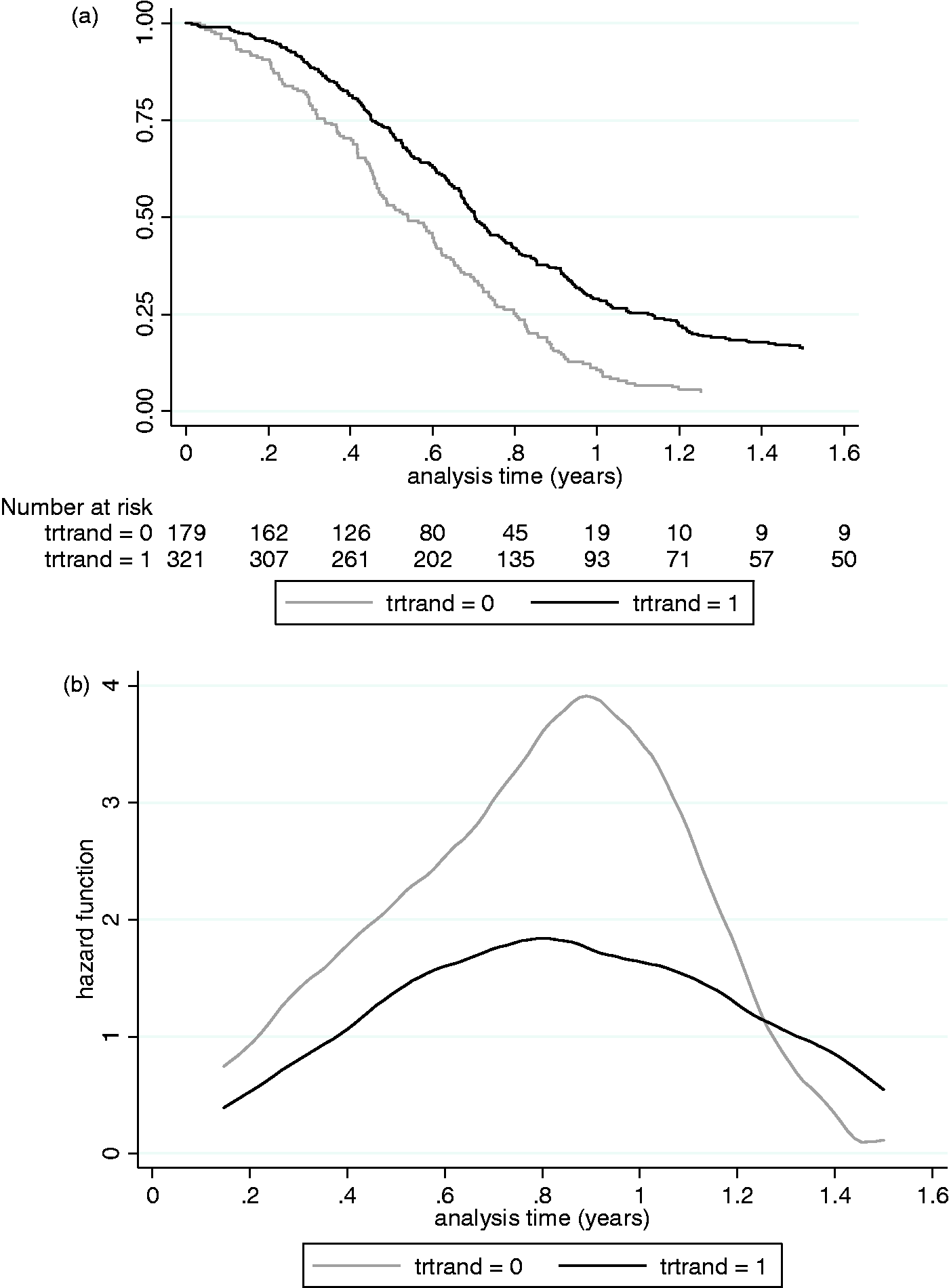

3.2 Treatment effect in the experimental group

We cannot summarise the treatment effect experienced in the experimental group using a single value, because our hazard function includes ‘t’ terms. As demonstrated by Figure 1(b), the treatment effect (as observed by the difference between the hazard functions) initially increases during the period of greatest hazard, before falling in the longer term. We believe that this is representative of a realistic treatment effect, which falls in the longer term when the initial treatment effect may have worn off, and when only better prognosis patients remain alive.

3.3 Treatment effect in switchers

The treatment effect applied to patients who switched from the control group to the experimental treatment was calculated in the same way as for our previous study. ² The baseline treatment effect was applied to switchers, but was multiplied by a factor (ω) such that the effect received was equal to or lower than the average effect received by experimental group patients. The magnitude of ω was varied across scenarios to represent relative reductions in the average treatment effect of 0 and 20%. This allowed us to test scenarios in which the ‘common treatment effect’ assumption did and did not hold.

3.4 The switching mechanism

Patients were only at risk of switching during the three consultations immediately following disease progression – switching was not permitted before disease progression had occurred, to reflect the treatment switching typically seen in metastatic cancer trials. ¹ In addition, switching was only permitted in patients who were randomly assigned a value of ‘1’ for a ‘choice’ variable. During this ‘at-risk’ period, the probability of switching declined for each individual patient with each simulated consultation, which were assumed to occur every 21 days. The probability of switching during the ‘at-risk’ period was calculated using a logistic function and depended upon the biomarker value at the time of disease progression and the time of progression itself. The probability of switching was highest if the biomarker value was high at the time of disease progression, and if time to progression was high. Both these factors indicate that patients with a relatively long progression-free survival period were more likely to switch. In the base case, switching probabilities were set such that approximately 40% of control group patients switched treatments. Switching probabilities were increased (or decreased) for all patients with a ‘choice’ covariate value of ‘1’ during their ‘at-risk’ period in order to investigate scenarios with higher (or lower) switching proportions. A variable for choice was incorporated because in most RCTs data on patient preference for switching are not collected, and for methods such as the IPCW this could represent an unmeasured confounder. Eighty per cent of patients were assigned a value of ‘1’ and 20% were assigned a value of ‘0’. Further details on the probability of switching in different simulated groups are presented in Appendix 1.

3.5 Scenarios investigated

The simulated data-generating mechanism had several variables for which values had to be assumed. These are listed in Appendix 2. The variables altered within our main set of scenarios related to:

Switch proportion: low (approximately 16% of control group), moderate (approximately 40% of control group);

Treatment effect: moderate (average HR under the incorrect assumption of proportional hazards, approximately 0.75), high (average HR approximately 0.50);

Relative treatment effect decrement received by switchers: 0%, 20%;

Severity of disease: moderate severity (restricted mean survival in control group approximately 365 days, administrative censoring proportion approximately 55%); severe (restricted mean survival in control group approximately 285 days, administrative censoring proportion approximately 15%);

Sample size: moderate (n = 500); small (n = 300), both with 2:1 randomisation in favour of the experimental treatment;

Data-generating model: two-component mixture Weibull baseline hazard function; two-component mixture Gompertz baseline hazard function.

Varying the switch proportion, the treatment effect size, the commonality of the treatment effect and disease severity resulted in 16 ‘base’ scenarios. Additionally, testing the impact of sample size and the data-generating model resulted in 64 scenarios. Finally, we re-ran four selected scenarios to replicate the high switching proportions simulated in our previous study, ² in order to assess the consistency of the results between the two studies. In total 68 scenarios were run. One thousand simulations were run for each scenario.

3.6 Performance measures

As was the case in our previous study, the time dependency of the treatment effect meant that it was not possible to produce a single ‘true’ HR or AF that the results of the adjustment methods could be compared to. Instead, we used restricted mean survival time as our true value upon which to base our performance measures. This is useful from a HTA perspective because for economic evaluation it is necessary to estimate mean survival times, in order that resource allocation decisions can be made based upon analyses that consider the impact of treating entire disease populations.

In our previous study, we were able to integrate the survivor functions associated with our simulated survival data in order to calculate the true restricted mean survival time for the control group for each scenario. However, the equation for the survival function was not analytically tractable in the current study. Instead, for each scenario we simulated data for 1,000,000 patients without incorporating treatment switching and estimated mean survival at 18 months (the administrative censoring time in the simulated datasets). We used this as the ‘truth’ upon which to base performance measures. Because this value is the product of a simulation rather than a calculation it is prone to error, but this is likely to be extremely minimal given the large number of patients simulated.

We evaluated the performance of the switching adjustment methods according to the bias in their estimate of the true survival (restricted mean at 18 months) for the control group. Bias (δ) was measured by the difference between the true restricted mean (β) and the estimated restricted mean ( $\overline{\hat{\beta }}$ ). Percentage bias was calculated as $\frac{\delta }{\beta }\times 100$ . ³⁴ The mean squared error (MSE) was also calculated to provide information on the variability of the estimates obtained using the different adjustment methods in combination with their bias. The standard error was that associated with the mean of the restricted means estimated by each adjustment method over the 1000 simulations run for each scenario.

The coverage of each method was also calculated, defined as the proportion of simulations where the 95% confidence intervals (CIs) of the restricted mean estimated by each method contained the true restricted mean. We also calculated the proportion of times that each method resulted in an estimate of the treatment effect (i.e. the proportion of times they converged). Where methods did not converge the bias and coverage performance measures were calculated based upon simulations in which convergence did occur.

3.7 Adjustment methods included

We included the following methods in the simulation study: ITT, Exclude switchers (PPexc), Censor at switch (PPcens), IPCW, IPCW excluding the ‘choice’ covariate (IPCWn), RPSFTM, IPE with a Weibull model (IPE), IPE with an exponential model (IPEexp), two-stage Weibull model (Weib2m), two-stage generalised Gamma model (Gam2m).

For the RPSFTM method, we used a Cox test within the g-estimation procedure, and for the IPE algorithm we tested the use of exponential and Weibull models within the estimation procedure, in order to assess whether the performance of the method is sensitive to this. The Stata command strbee was used to apply the RPSFTM and IPE methods, ³⁵ and baseline covariates were included in the models. For the IPCW method, we used stabilised weights used a similar approach to that described by Fewell et al.³⁶ We included two versions – one in which all covariates were included in the relevant models, and one in which the ‘choice’ covariate was excluded – in order to test the sensitivity of the method to the availability of this covariate.

We applied the two-stage method using Weibull and generalised Gamma models, so that the performance of different AFT models could be compared. We fitted these models to control group patients using disease progression as the secondary baseline time point, and included covariates for switching, baseline prognosis group, baseline biomarker value, time-to-disease progression, biomarker value at disease progression and the ‘choice’ covariate.

It has been shown that informative censoring is problematic for adjustment methods that estimate counterfactual survival times,^37–39 and therefore RPSFTM, IPE and two-stage methods incorporated recensoring, whereby the counterfactual survival time $U_i(\psi )$ was recensored at the minimum of the administrative censoring time C_i and $C_i\text{exp}\psi$ . $U_i(\psi )$ was then replaced by the censoring time of the counterfactual event time $D_i^{*}(\psi )$ if $D_i^{*}(\psi )<U_i(\psi )$ .

For each of the methods applied, the techniques used to derive mean survival times restricted to 18 months were similar to those used in our previous study. ² For the ITT, PPexc and PPcens analyses, Stata’s stci command was used to calculate the area under the Kaplan–Meier survivor function at 18 months for the specified group. For the IPCW, RPSFTM, IPE and two-stage estimation analyses, the ‘survivor function’ approach was used. ² First, the inverse of the estimated treatment effect was applied to the experimental group hazard function (modelled using a flexible parametric model) to obtain the adjusted control group hazard function. For the IPCW methods, the treatment effect used was the IPCW HR, and for the RPSFTM, IPE and two-stage methods, the HR associated with the adjustment (estimated using a flexible parametric model comparing observed experimental group survival times and adjusted control group survival times) was used. From this, the control group survivor function was derived, allowing mean survival at 18 months to be calculated. CIs were derived in the same way, except the inverse of the 95% CIs of the estimated treatment effect were applied to the experimental group hazard function.

4 Results

We present detailed results from eight scenarios that illustrate the key findings. First we report key results in scenarios that involved moderate (approximately 50%) switching proportions, followed by key results in scenarios that involved low (approximately 20%) switching proportions. We then summarise the extent to which the eight scenarios focussed upon reflect the results of the eight other base scenarios completed. Finally, we summarise the results of the additional scenarios run – those that tested the sensitivity of the results to the sample size, the data-generating model and those that tested extreme high switching proportions.

A summary table describing the characteristics of each scenario is presented in Appendix 3, and Appendix 4 presents the percentage bias for each adjustment method across all scenarios.

4.1 Scenarios with moderate switching proportions

Tables 1 and 2 present detailed results from Scenarios 1, 3, 9 and 11. These are illustrative of the results of scenarios in which the switching proportion simulated was approximately 58–61% of at-risk patients (30–44% of all control group patients).

Table 1.

Scenarios 1 and 3 – results.

Scenario details	Method	Mean estimate	SE of mean	95% Confidence interval		Bias	Percent bias	MSE	Coverage (%)	Successful estimation (%)
				Lower	Upper
Scenario number: 1 True mean survival: Control: 0.56 Experimental: 0.79 Mean switch: 58.26% True ave. HR: 0.51 Mean censored: 13.59% Treatment effect: 20% decrement	ITT	0.60	0.03	0.55	0.66	0.05	8.22	0.0029	65.40	100.00
	PPExc	0.50	0.04	0.43	0.58	-0.06	-9.94	0.0044	66.40	100.00
	PPcens	0.65	0.04	0.57	0.74	0.10	17.66	0.0114	36.10	100.00
	IPCW	0.54	0.03	0.47	0.63	-0.01	-2.30	0.0013	97.60	100.00
	IPCWn	0.54	0.03	0.47	0.63	-0.01	-2.46	0.0012	97.40	100.00
	Weib2m	0.56	0.03	0.54	0.58	0.00	0.62	0.0009	55.60	100.00
	Gam2m	0.56	0.03	0.54	0.58	0.00	0.54	0.0009	56.30	100.00
	RPSFTM	0.55	0.03	0.49	0.62	-0.01	-1.40	0.0011	94.70	100.00
	IPE	0.55	0.03	0.48	0.62	-0.01	-1.70	0.0012	94.20	100.00
	IPEexp	0.55	0.03	0.48	0.62	-0.01	-1.90	0.0012	93.90	100.00
Scenario number: 3 True mean survival: Control: 0.64 Experimental: 0.74 Mean switch: 61.20% True ave. HR: 0.76 Mean censored: 15.03% Treatment effect: 20% decrement	ITT	0.66	0.03	0.60	0.72	0.02	2.94	0.0014	91.90	100.00
	PPExc	0.61	0.05	0.51	0.70	-0.03	-5.37	0.0034	86.50	100.00
	PPcens	0.78	0.05	0.69	0.88	0.14	22.13	0.0223	14.70	100.00
	IPCW	0.65	0.04	0.55	0.76	0.01	1.19	0.0018	98.40	100.00
	IPCWn	0.64	0.04	0.55	0.74	0.00	0.51	0.0015	98.60	100.00
	Weib2m	0.64	0.03	0.61	0.67	-0.00	-0.42	0.0012	52.60	100.00
	Gam2m	0.64	0.03	0.61	0.67	-0.00	-0.52	0.0012	53.70	99.90
	RPSFTM	0.63	0.04	0.56	0.71	-0.01	-1.40	0.0018	93.30	100.00
	IPE	0.63	0.04	0.56	0.71	-0.01	-1.69	0.0019	92.80	100.00
	IPEexp	0.63	0.04	0.56	0.71	-0.01	-1.79	0.0019	92.50	100.00

Table 2.

Scenarios 9 and 11 – results.

Scenario details	Method	Mean estimate	SE of mean	95% Confidence interval		Bias	Percent bias	MSE	Coverage (%)	Successful estimation (%)
				Lower	Upper
Scenario number: 9 True mean survival: Control: 0.56 Experimental: 0.79 Mean switch: 58.27% True ave. HR: 0.51 Mean censored: 13.74% Treatment effect: 0% decrement	ITT	0.61	0.03	0.55	0.67	0.05	9.83	0.0039	56.20	100.00
	PPExc	0.50	0.04	0.42	0.57	-0.06	-10.54	0.0049	63.40	100.00
	PPcens	0.65	0.04	0.57	0.74	0.10	17.16	0.0109	40.10	100.00
	IPCW	0.54	0.03	0.47	0.63	-0.01	-2.27	0.0013	98.00	100.00
	IPCWn	0.54	0.03	0.47	0.63	-0.01	-2.49	0.0012	97.70	100.00
	Weib2m	0.56	0.03	0.54	0.58	0.00	0.48	0.0009	55.90	100.00
	Gam2m	0.56	0.03	0.54	0.58	0.00	0.42	0.0009	56.70	100.00
	RPSFTM	0.56	0.04	0.49	0.63	0.00	-0.01	0.0012	95.10	100.00
	IPE	0.55	0.03	0.49	0.63	0.00	-0.31	0.0012	95.30	100.00
	IPEexp	0.55	0.03	0.49	0.62	0.00	-0.55	0.0012	94.90	100.00
Scenario number: 11 True mean survival: Control: 0.64 Experimental: 0.74 Mean switch: 60.90% True ave. HR: 0.76 Mean censored: 15.09% Treatment effect: 0% decrement	ITT	0.66	0.03	0.60	0.73	0.02	3.48	0.0016	89.10	100.00
	PPExc	0.61	0.05	0.51	0.70	-0.04	-5.46	0.0036	84.60	100.00
	PPcens	0.78	0.05	0.69	0.88	0.14	21.74	0.0218	16.20	100.00
	IPCW	0.65	0.04	0.55	0.76	0.01	1.29	0.0020	98.00	100.00
	IPCWn	0.65	0.04	0.55	0.74	0.00	0.60	0.0017	98.30	100.00
	Weib2m	0.64	0.04	0.61	0.66	-0.00	-0.61	0.0013	51.30	100.00
	Gam2m	0.64	0.04	0.61	0.66	-0.00	-0.71	0.0013	51.20	100.00
	RPSFTM	0.64	0.04	0.56	0.72	0.00	-0.77	0.0020	92.10	100.00
	IPE	0.63	0.04	0.56	0.71	-0.01	-1.06	0.0020	91.20	100.00
	IPEexp	0.63	0.04	0.56	0.71	-0.01	-1.17	0.0021	90.70	100.00

The characteristics of Scenario 1, with regard to survival times, switch proportion, treatment effect and censoring proportion are described in Table 1. To summarise, this scenario incorporated a moderate switch proportion, a large treatment effect, a low censoring proportion and violated the common treatment effect assumption. It is important to note that the average HR is included in Tables 1 to 4 for illustrative purposes only, to give an idea of the size of the treatment effect – it was estimated by generating scenario-specific survival data for a large number of patients (1,000,000) without applying switching, and by fitting a Cox model to this. However, given that the proportional hazards assumption does not apply in our simulated datasets, this estimate of the treatment effect is prone to error.

Table 3.

Scenarios 5 and 7 – results.

Scenario details	Method	Mean estimate	SE of mean	95% Confidence interval		Bias	Percent bias	MSE	Coverage (%)	Successful estimation (%)
				Lower	Upper
Scenario number: 5 True mean survival: Control: 0.56 Experimental: 0.79 Mean switch 23.78% True ave. HR: 0.51 Mean censored: 13.42% Treatment effect: 20% decrement	ITT	0.58	0.03	0.52	0.63	0.02	3.47	0.0011	90.00	100.00
	PPExc	0.53	0.03	0.47	0.59	-0.03	-4.76	0.0016	83.60	100.00
	PPcens	0.58	0.03	0.52	0.64	0.02	4.18	0.0015	89.90	100.00
	IPCW	0.54	0.03	0.47	0.61	-0.02	-3.52	0.0012	95.80	100.00
	IPCWn	0.54	0.03	0.47	0.61	-0.02	-3.53	0.0012	95.40	100.00
	Weib2m	0.56	0.03	0.55	0.58	0.01	1.02	0.0008	35.10	100.00
	Gam2m	0.56	0.03	0.55	0.58	0.01	1.03	0.0008	36.50	100.00
	RPSFTM	0.56	0.03	0.49	0.63	0.00	-0.17	0.0008	97.90	100.00
	IPE	0.55	0.03	0.49	0.63	0.00	-0.31	0.0008	97.90	100.00
	IPEexp	0.55	0.03	0.49	0.63	0.00	-0.33	0.0008	98.10	100.00
Scenario number: 7 True mean survival: Control: 0.64 Experimental: 0.74 Mean switch: 25.87% True ave. HR: 0.76 Mean censored: 15.15% Treatment effect: 20% decrement	ITT	0.65	0.03	0.59	0.72	0.01	1.69	0.0012	94.50	100.00
	PPExc	0.62	0.04	0.55	0.69	-0.02	-3.10	0.0018	88.70	100.00
	PPcens	0.68	0.04	0.61	0.75	0.04	6.19	0.0029	82.00	100.00
	IPCW	0.64	0.04	0.56	0.73	0.00	-0.15	0.0014	98.20	100.00
	IPCWn	0.64	0.04	0.56	0.73	0.00	-0.21	0.0014	98.10	100.00
	Weib2m	0.65	0.03	0.63	0.66	0.00	0.63	0.0012	33.50	100.00
	Gam2m	0.65	0.03	0.63	0.66	0.00	0.59	0.0012	33.60	100.00
	RPSFTM	0.64	0.04	0.57	0.72	0.00	-0.17	0.0014	96.80	100.00
	IPE	0.64	0.04	0.56	0.72	0.00	-0.29	0.0014	96.40	100.00
	IPEexp	0.64	0.04	0.56	0.72	0.00	-0.30	0.0014	96.50	100.00

Table 4.

Scenarios 13 and 15 – results.

Scenario details	Method	Mean estimate	SE of mean	95% Confidence interval		Bias	Percent bias	MSE	Coverage (%)	Successful estimation (%)
				Lower	Upper
Scenario number: 13 True mean survival: Control: 0.56 Experimental: 0.79 Mean switch: 23.76% True ave. HR: 0.51 Mean censored: 13.52% Treatment effect: 0% decrement
	ITT	0.58	0.03	0.52	0.63	0.02	3.99	0.0013	88.40	100.00
	PPExc	0.53	0.03	0.47	0.59	-0.03	-5.19	0.0017	80.80	100.00
	PPcens	0.58	0.03	0.52	0.64	0.02	3.73	0.0014	90.90	100.00
	IPCW	0.53	0.03	0.47	0.61	-0.02	-4.02	0.0014	94.90	100.00
	IPCWn	0.53	0.03	0.47	0.61	-0.02	-4.05	0.0014	95.00	100.00
	Weib2m	0.56	0.03	0.55	0.57	0.00	0.60	0.0008	31.00	100.00
	Gam2m	0.56	0.03	0.55	0.57	0.00	0.58	0.0008	31.70	99.70
	RPSFTM	0.56	0.03	0.49	0.63	0.00	0.11	0.0009	97.90	100.00
	IPE	0.56	0.03	0.49	0.63	0.00	0.01	0.0009	97.90	100.00
	IPEexp	0.56	0.03	0.49	0.63	0.00	-0.06	0.0009	98.20	100.00
Scenario number: 15 True mean survival: Control: 0.64 Experimental: 0.74 Mean switch: 25.61% True ave. HR: 0.76 Mean censored: 15.04% Treatment effect: 0% decrement	ITT	0.65	0.03	0.59	0.71	0.01	1.43	0.0011	94.90	100.00
	PPExc	0.62	0.04	0.55	0.69	-0.02	-3.68	0.0019	89.10	100.00
	PPcens	0.68	0.04	0.60	0.75	0.04	5.51	0.0025	86.20	100.00
	IPCW	0.64	0.04	0.56	0.72	0.00	-0.76	0.0013	97.70	100.00
	IPCWn	0.64	0.04	0.56	0.72	-0.01	-0.83	0.0013	97.80	100.00
	Weib2m	0.64	0.03	0.63	0.66	0.00	0.02	0.0011	33.50	100.00
	Gam2m	0.64	0.03	0.63	0.66	-0.00	-0.00	0.0011	33.10	99.70
	RPSFTM	0.64	0.04	0.56	0.72	0.00	-0.45	0.0013	96.50	100.00
	IPE	0.64	0.04	0.56	0.72	0.00	-0.55	0.0013	96.40	100.00
	IPEexp	0.64	0.04	0.56	0.72	0.00	-0.58	0.0013	96.40	100.00

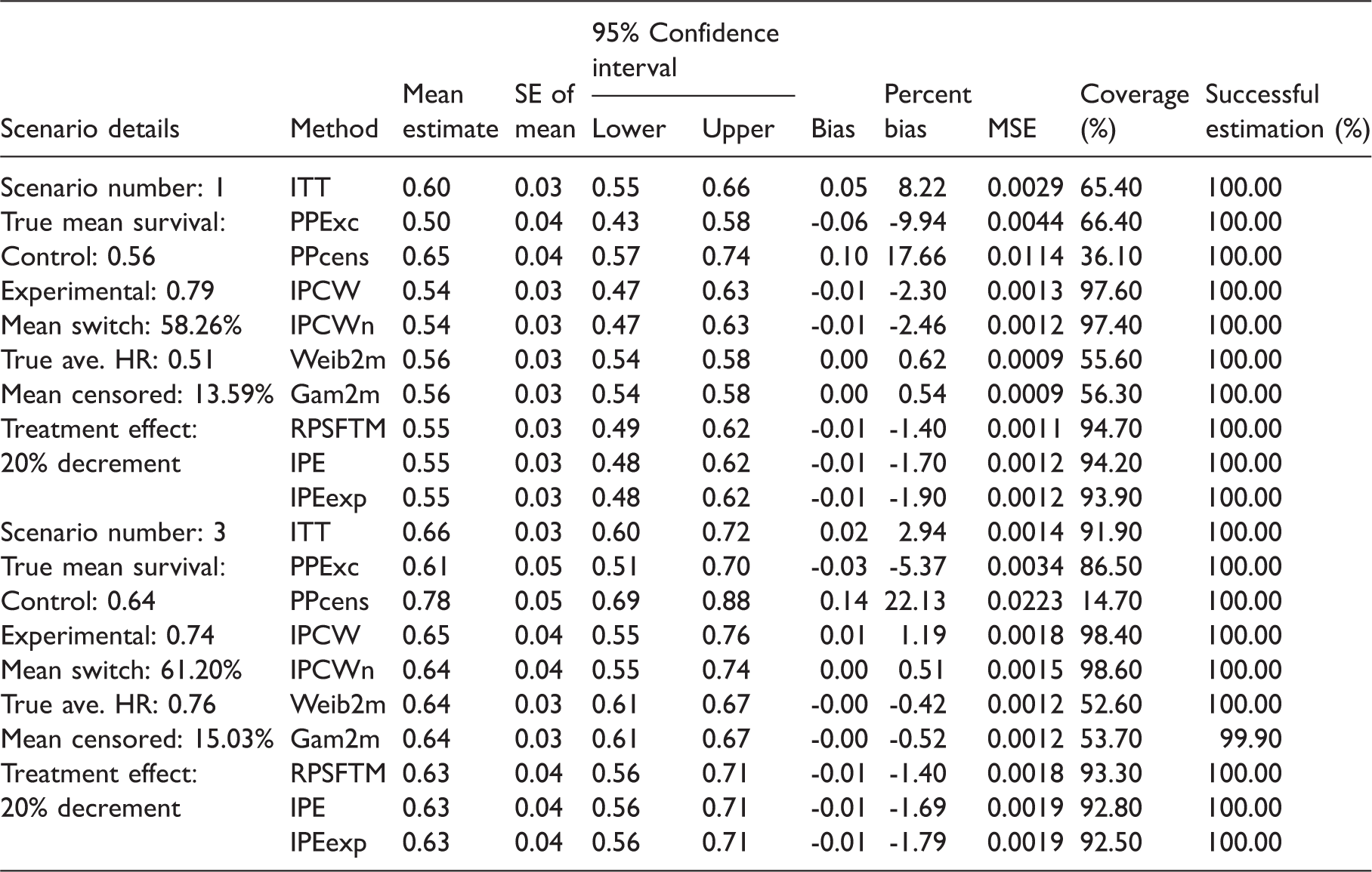
As expected, in Scenario 1 the ITT analysis overestimated the true, unconfounded control group restricted mean survival time, equivalent to a percentage bias of 8.22%. Simple adjustment methods (PPexc, PPcens) produced substantially higher percentage bias than the ITT analysis. The IPCW and the IPCWn both underestimated mean survival in the control group (hence over-estimated the treatment effect) but produced lower bias than the ITT analysis (percentage bias -2.30 and -2.46% for IPCW and IPCWn, respectively). The RPSFTM, IPE and IPEexp produced similarly low levels of bias (percentage bias -1.40, -1.70 and -1.90%, respectively), under-estimating mean survival in the control group but producing lower bias than the ITT and IPCW analyses. The Weib2m and Gam2m methods produced less bias than all other methods, resulting in very low percentage bias of 0.62 and 0.54%, respectively.

The only substantive difference between Scenario 1 and Scenario 3 was that the treatment effect was smaller in Scenario 3 (see Table 2). Due to this, the relative bias associated with each of the adjustment methods generally marginally decreased. However, the best performing adjustment methods remained the same – the Weib2m and Gam2m produced least bias (percentage bias -0.42 and -0.52%, respectively). In contrast, in this scenario the IPCW and IPCWn produced lower bias than the RPSFTM, IPE and IPEexp (percentage bias 1.19 and 0.51% compared to -1.40, -1.69 and -1.79%, respectively). The simple adjustment methods again produced substantially higher levels of bias. Due to the lower treatment effect the ITT analysis produced lower percentage bias than in Scenario 1, but still produced higher bias than all adjustment methods except PPcens and PPexc.

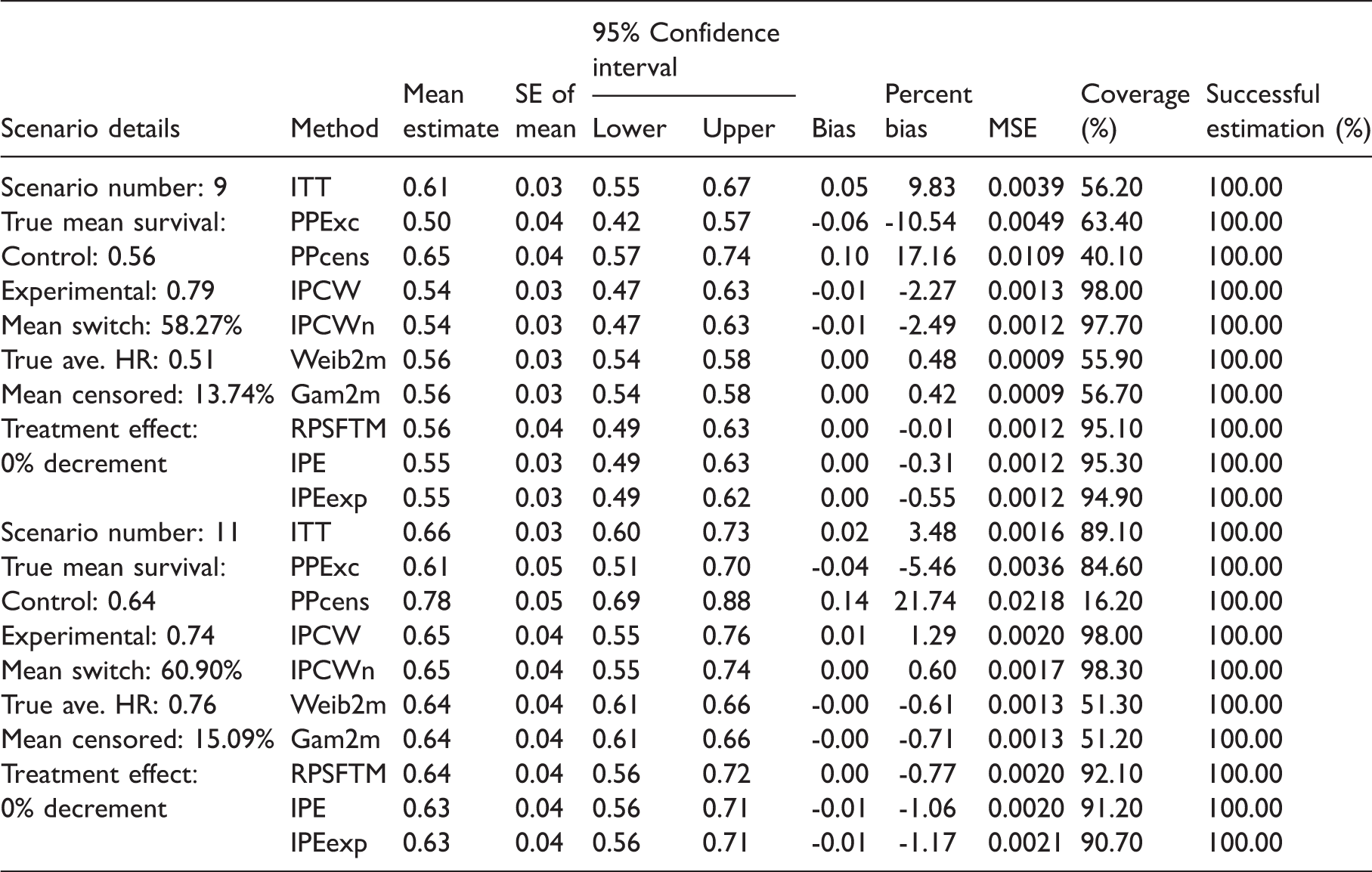
Table 2 presents detailed results of Scenario 9 and Scenario 11. Scenario 9 is approximately equivalent to Scenario 1 and Scenario 11 is approximately equivalent to Scenario 3, except the common treatment effect assumption holds. This has an important impact upon the results of the randomisation-based adjustment methods. While the Weib2m and Gam2m methods continued to produce similarly low levels of bias, the percentage bias associated with the RPSFTM/IPE methods reduced. The IPCW and IPCWn methods produced similar levels of bias to those found in Scenarios 1 and 3. The ITT analysis again produced higher bias than all adjustment methods except PPcens and PPexc.

Tables 1 and 2 show a substantial difference in the levels of coverage and MSE achieved by each of the adjustment methods. It is important to note the low levels of coverage achieved by the Weib2m and Gam2m (ranging from 51.20 to 56.70%) – particularly because these produce low levels of bias. In contrast, the IPCW method produced higher levels of coverage (97.40–98.60%) in Scenarios 1, 3, 9 and 11, indicating relatively wide CIs. The RPSFTM, IPE and IPEexp approaches led to similarly high levels of coverage (ranging from 90.70 to 95.30%).

The two-stage adjustment methods also produced poor coverage in our previous study, ² because CIs for mean counterfactual survival times were estimated by using the 95% CIs for ${\psi }^0$ in equation (2). This only takes into account the uncertainty in the treatment effect itself – it does not take into account the uncertainty in the underlying survival distribution. In reality, if a two-stage approach were to be taken, uncertainty around mean survival estimates would need to be taken into account using bootstrapping.

The MSE results suggest that the levels of variability associated with the different adjustment methods were generally similar relative to the bias levels – i.e. higher levels of bias were generally associated with higher MSEs.

Successful estimation was achieved with all of the adjustment methods across Scenarios 1, 3, 9 and 11, with the Gam2m method failing to converge in 0.1% of simulations in Scenario 3. The IPCW and IPCWn methods failed to converge in one of the weighting regressions in several simulations, but estimations were still obtained from these. Restricting the results of these methods only to simulations in which full convergence was achieved in each of the regression models had only a minor impact on their performance – as described in Appendix 5.

4.2 Scenarios with low switching proportions

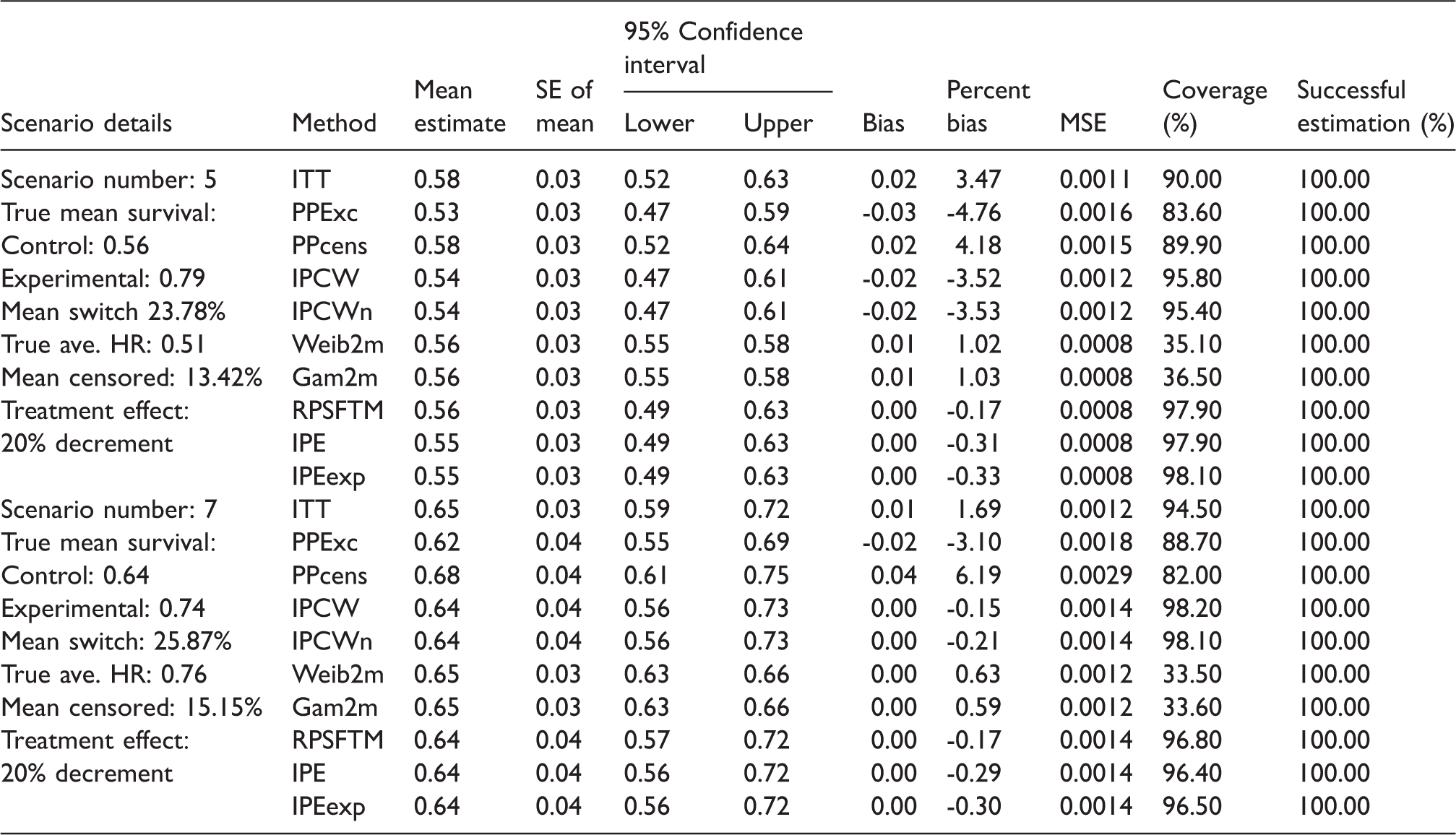
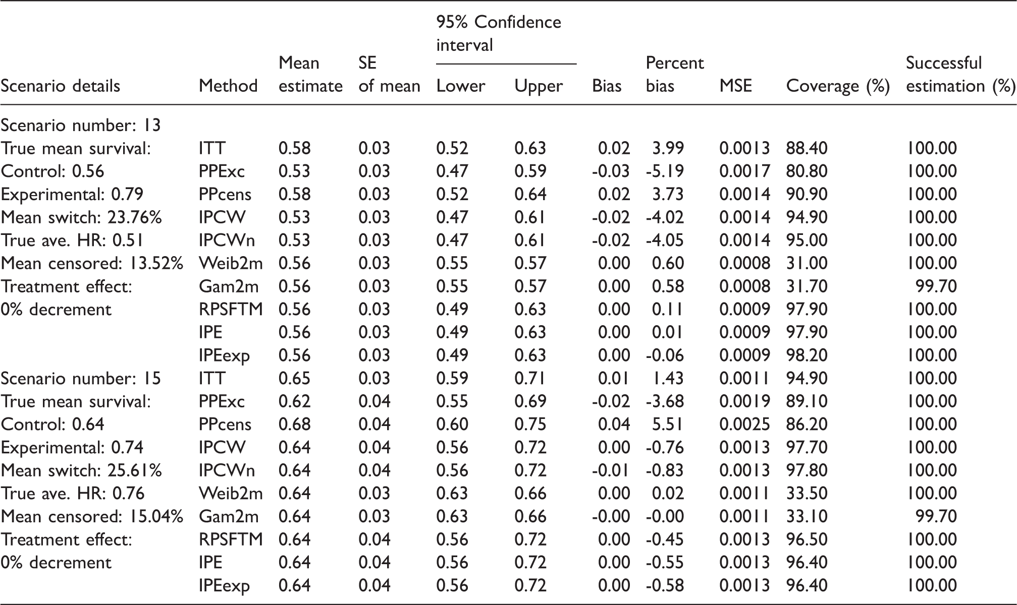
Tables 3 and 4 present detailed results from Scenarios 5, 7, 13 and 15. These are illustrative of the results of scenarios in which the switching proportion simulated was approximately 23–26% of at-risk patients (13–18% of the control group as a whole). Scenarios 5, 7, 13 and 15 are similar to Scenarios 1, 3, 9 and 11, respectively, with the only substantive difference the switching proportion.

The reduced switching proportion has a limited impact on the bias, coverage and convergence associated with the adjustment methods. The bias associated with the IPCW methods seemed slightly more sensitive to the reduction in the switching proportion than the other adjustment methods: in Scenarios 7 and 15 the bias associated with the IPCW and IPCWn methods decreased compared to Scenarios 3 and 11, whereas in Scenarios 5 and 13 the opposite was true compared to Scenarios 1 and 9. The percentage bias of the Weib2m and Gam2m methods generally marginally increased in these scenarios and coverage remained poor. The percentage bias of the RPSFTM/IPE methods generally marginally reduced and coverage improved, suggesting that the performance of these methods is improved in scenarios with lower switching proportions. All complex adjustment methods continued to produce lower bias than the ITT analysis, with the exception of the IPCW and IPCWn methods, which produced marginally more bias than the ITT analyses in Scenarios 5 and 13.

4.3 Other base scenarios

The results presented in Sections 4.1 and 4.2 provide a clear illustration of our key findings. Across all of these scenarios the complex adjustment methods generally performed well, with percentage bias usually below 1.0%, with the possible exception of the IPCW and IPCWn methods in scenarios where the treatment effect is high (in which percentage bias increased to ± 2–4%).

In the other base scenarios (i.e. the first 16 scenarios detailed in Appendix 3) the pattern of the results remained similar – PPcens and PPexc approaches generated very high levels of bias; RPSFTM, IPE and IPEexp methods produced low bias – in particular when the ‘common treatment effect’ assumption held; the Weib2m and Gam2m methods produced generally low levels of bias across all scenarios; IPCW and IPCWn methods generally produced lower levels of bias than the ITT analysis and sometimes produced similar levels of bias to the RPSFTM, IPE and IPEexp methods in scenarios where the common treatment effect assumption did not hold, but percentage bias fluctuated more between scenarios. Percentage bias is presented for each method across each of the scenarios in Appendix 4.

Across Scenarios 1–16 the percentage bias associated with the RPSFTM, IPE and IPEexp methods generally more than doubled in scenarios where the common treatment effect assumption did not hold. In contrast, percentage bias was approximately quartered in scenarios where the switching proportion was reduced from 30 to 44% of the control group to 13–18%.

It is notable that in all scenarios the RPSFTM, IPE and IPEexp methods led to negative bias – that is they over-adjusted for the treatment switching effect. Such a pattern was not clear for the IPCW, IPCWn, Weib2m and Gam2m methods, with bias fluctuating between positive and negative.

For the IPCW and IPCWn, the switching proportion and the size of the treatment effect were the most important factors for performance. Appendix 4 illustrates that for the IPCW, percentage bias generally reduced when the switching proportion was reduced from 30 to 44% of the control group (equivalent to approximately 60% of ‘at-risk’ patients) to 13–18% (equivalent to approximately 25% of ‘at-risk’ patients) (compare Scenarios 1–4 and 9–12 to Scenarios 5–8 and 13–16) – although this pattern was not wholly consistent. Percentage bias also reduced in scenarios where the treatment effect was reduced (Scenarios 3, 4, 7, 8, 11, 12, 15 and 16 compared to Scenarios 1, 2, 5, 6, 9, 10, 13 and 14). The IPCW and IPCWn methods usually produced higher levels of bias than the randomisation-based methods, although this was often only marginal. Across Scenarios 1–8, in which the common treatment effect assumption did not hold, the IPCW and IPCWn methods produced lower bias than the RPSFTM in three.

The two-stage adjustment methods (Weib2m and Gam2m) were less sensitive to the scenario parameters than the other adjustment methods, with neither the switch proportion nor the treatment effect substantially affecting bias across Scenarios 1–16.

Across Scenarios 1–16, the Gam2m method produced least percentage bias in six scenarios, and the Weib2m produced least percentage bias in three scenarios. The RPSFTM produced least percentage bias in four scenarios and the IPE produced least percentage bias in one scenario. The IPCW and IPCWn methods produced least percentage bias in one scenario apiece. The ITT, PPexc and PPcens never produced least percentage bias.

4.4 Impact of sample size

Scenarios 17–32 replicated Scenarios 1–16, but with the sample size simulated in each scenario reduced to 300. We anticipated that this would cause a worsening in the performance of the adjustment methods, particularly for the IPCW and IPCWn due to their observational basis. As illustrated by Appendix 4, in fact, there was a marginal increase in bias for all methods, and the increase was not substantially greater for the IPCW approaches when compared to the RPSFTM, IPE and IPEexp. Coverage in Scenarios 1–16 and Scenarios 17–32 was similar, with a marginal increase in the scenarios with smaller sample size, reflecting slightly wider CIs. Reduced sample size led to convergence problems for the IPCW, IPCWn and Gam2m methods, with convergence of the Gam2m falling to 88.1% in these scenarios (compared to 98.8% in Scenarios 1–16).

4.5 Impact of disease severity

Scenarios with an odd number simulated a severe disease and an administrative censoring proportion of approximately 15%, whereas scenarios with an even number simulated moderate disease, with an administrative censoring proportion of approximately 55%. It was difficult to identify the specific effect that increases in disease severity and changing censoring proportions had on the performance of the adjustment methods, because a consequence of a decreased disease severity and an increased censoring proportion was that a lower number of control group patients were simulated to switch treatments – which itself is likely to influence method performance. However, for most of the complex adjustment methods (with the exception of the IPCWn, Weib2m and Gam2m) percentage bias generally marginally increased in scenarios with lower disease severity and consequent higher censoring proportions, despite the lower overall switching proportion in these scenarios. For the IPCW, IPCWn and particularly for the Gam2m there was a trend towards marginally poorer convergence in scenarios with lower disease severity and higher censoring proportions.

4.6 Impact of the data generation model

Scenarios 33–64 replicated Scenarios 1–32, replacing the two-component mixture Weibull baseline hazard function data generation model with a two-component mixture Gompertz baseline hazard function data generation model. Apart from the underlying hazard function, these scenarios were similar (see Appendix 3 for details). We found that the performance of the adjustment methods in Scenarios 33–64 was very similar to that observed in Scenarios 1–32.

4.7 Extreme switching proportions

Scenarios 65–68 replicated Scenarios 1–4, but incorporated a very high switching proportion (47–70% of all control group patients, equivalent to 94–95% of ‘at-risk’ patients). The extreme increase in switching proportion increased the bias associated with all adjustment methods, as illustrated in Appendix 4. This increase was much more substantial for the IPCW method than all other methods, and in three of the four scenarios the IPCW method produced more bias than the ITT analysis. Notably, the percentage bias associated with the IPCWn method did not increase substantially in Scenarios 65–68. This is because the IPCWn method does not take into account the ‘choice’ covariate, whereas the IPCW method does. In Scenarios 65–68, the number of control group patients who were at risk of switching but did not switch ranged between 4 and 8 for the IPCW method, whereas for the IPCWn method this number ranged between 25 and 40 because all control group patients were included in the risk set, rather than only those with a ‘choice’ covariate value of ‘1’. The results of Scenarios 65–68, and those of our previous study, ² demonstrate that the IPCW method is prone to substantial error when the switching proportion amongst those at risk of switching is very high (in excess of 90%), leaving very few at-risk patients who do not switch: in Scenarios 65–68, this was the case for the risk set defined by the IPCW method, but not for the risk set defined by the IPCWn method. In fact, in these scenarios, the IPCWn method produced least percentage bias in two of the four scenarios, with the Weib2m method producing least percentage bias in the remaining two scenarios.

5 Discussion

Our simulation study demonstrates that complex statistical adjustment methods produce low bias in a wide range of scenarios, provided switching proportions are low or moderate. The complex adjustment methods produced estimates of the comparative treatment effect that were closer to the truth than the ITT analysis, whilst the naïve adjustment methods produced substantially higher levels of bias. In general, the results of the current study support the findings of our previous study. ² However, important new information has been obtained. In particular, by comparing the results of the current study with those of our previous study, we can show that it is important to assess the magnitude of the average treatment effect in terms of an AF rather than a HR. In general, the current study has provided more information on the key factors that influence the performance of adjustment methods; this can be used to assist in the process of determining which adjustment methods are likely to be appropriate on a case-by-case basis. These issues are discussed below.

In our previous study we often found levels of percentage bias of between 5 and 10%, or even higher in scenarios with high switching proportions or where the common treatment effect assumption did not hold. ² In the current study, levels of percentage bias rarely exceeded 2–3% across all scenarios except those that incorporated extreme switching proportions. This is partly because in our previous study half of the 72 scenarios run included extremely high switching proportions, compared to only four scenarios in the current study. However, we believe this is also due to the different data-generating mechanism used in the current study, which led to different survival time distributions and different treatment effects when measured on the AFT scale.

Although we cannot summarise the treatment effect simulated in either of our studies by a single value, because the treatment effect varies as a function of time, we can estimate what the HR or AF would be assuming proportional hazards or a constant AF, even though neither of these assumptions is true in our simulation models. Taking this approach, we find that we simulated similar average HRs in the two studies, but average AFs were very different. For example, in our previous study the average AF across the 72 scenarios varied between 1.44 and 3.58 and was over 2.0 in 60 of the 72 scenarios. In the current study, the AF across Scenarios 1–32 ranged between 1.22 and 1.78. This is of importance for two reasons. First, the performance of each of the adjustment methods is affected by the size of the treatment effect – particularly the IPCW methods, which produce more bias when the treatment effect is higher. Therefore, the lower biases found in the current study may be expected. Second, in the scenarios that violated the common treatment effect assumption, the decrement in the treatment effect received by switchers was calculated as a proportion of the average AF in the experimental group. When this AF is lower, a lower absolute decrement in the treatment effect will be applied to switchers, given the same proportional decrement. This is highly likely to explain why the randomisation-based methods were much less sensitive to departures from the common treatment effect assumption in the current study – it is the absolute difference in the AF between switchers and patients randomised to the experimental group that determines the subsequent bias of these methods. Generally, treatment effects in clinical trials are estimated in terms of a HR, but, our results show that when assessing the potential bias associated with the application of adjustment methods, it is important to also assess the size of the treatment effect in terms of an AF.

Whilst the current study suggests that complex statistical methods to adjust for treatment switching are generally stable and prone to low levels of bias in situations when switching proportions are moderate or low, within these scenarios important variations in the performance of methods arise – and the optimal adjustment method changes. Simple adjustment methods (PPexc and PPcens) should be avoided, since these produce higher bias than all of the other adjustment methods and the ITT analysis across all scenarios. The Gam2m and Weib2m generally produced least bias, unless the common treatment effect assumption held and the switching proportion was low, in which case the RPSFTM, IPE and IPEexp methods were often preferable. Taking the results of the current study together with the results of our previous study, ² we know that the randomisation-based methods are prone to higher levels of bias when the common treatment effect assumption does not hold, and when the AF associated with the new treatment is relatively high (for instance, greater than 2.0). We also know that the two-stage adjustment method is well suited to the scenarios simulated, because switching always occurred relatively soon after the disease progression secondary baseline. Our study results suggest that in real-world situations the randomisation-based methods and two-stage approach should be preferred when they are well suited to the characteristics of the trial under investigation. Where the common treatment effect assumption is implausible, the AF is high and there is no suitable secondary baseline, the IPCW method represents an adjustment method that is likely to produce lower bias than the ITT analysis, provided the switching proportion is not extreme (greater than 20 ‘at-risk’ patients remain ‘unswitched’) and no important prognostic covariates are missing.

However, circumstances remain in which adjustment methods may not improve upon the ITT analysis, particularly if we consider the results of the present study alongside those of our previous study.

In the current study, the IPCW and IPCWn methods produced less bias than the ITT analysis in 70 and 75% of scenarios, respectively, excluding the four scenarios in which the switching proportion was extremely high – in which the IPCW method performed poorly. The ITT analysis produced less bias than the IPCW and IPCWn methods in some scenarios in which the administrative censoring proportion was high (causing the adjustment methods to work slightly less well) combined with a relatively low treatment effect (meaning the bias associated with the ITT was relatively low), or when the treatment effect was higher (which led to more bias in the IPCW analyses) combined with a low switching proportion (which led to less bias in the ITT analysis). When attempting to determine whether an IPCW analysis is likely to provide less bias than an ITT analysis in reality, a combination of factors must be taken into account, including data availability, switching proportion, treatment effect size and censoring proportion. When applying the IPCW, it should also be noted that it is only necessary to include covariates that predict switching and survival. The current study showed that there was no appreciable advantage to including the ‘choice’ covariate in the IPCW analysis, and in fact this led to substantially more bias when extreme proportions switched. Including additional covariates increases the likelihood of obtaining extreme weights and does not improve the performance of the adjustment if the additional covariates are not prognostic. In addition, it should be considered that the IPCW approach does not take into account events that may occur outside the trial in question, which could influence the probability of switching within the trial. For instance, new evidence on the effectiveness of a similar treatment in a particular group of patients may alter the pattern of switching in the trial in question, which could affect the ability of the method to accurately predict the probability of switching.

The randomisation-based methods produced less bias than the ITT analysis across all scenarios in the current study, despite the inclusion of scenarios that violated the common treatment effect assumption. This is an important result that should increase confidence in these methods. However, this should be interpreted with some caution, given that our previous study demonstrated that when the AF is high (greater than 2.0) the potential for bias due to violations of the common treatment effect assumption is much greater. Hence, the size of the AF and the plausibility of the common treatment effect assumption must be investigated when considering the use of these methods. In addition, it should be noted that these methods produce decreased bias when the switching proportion is low.

The two-stage adjustment methods produced less bias than the ITT analysis in 93% of the scenarios included in the current study, often produced least bias of all the adjustment methods and were much less sensitive to the scenario parameters than the other adjustment methods. The Gam2m method generally produced marginally lower bias than the Weib2m – which may be expected given the greater flexibility of the three-parameter generalised Gamma model – but experienced some convergence issues when the sample size was 300, and when the proportion of administrative censoring was high. In practice, the AFT model used within the two-stage estimation method should be determined through a consideration of which model best fits the data. The two-stage adjustment methods were less likely to produce least bias in scenarios in which the common treatment effect assumption held and there was a lower switching proportion – in these scenarios it was more common for the randomisation-based methods to produce least bias. Therefore, again, several trial characteristics must be taken into account when considering the utility of applying two-stage adjustment methods to trials affected by treatment switching.

Based upon our study, it is not possible to predict the direction of bias associated with the adjustment methods. The randomisation-based methods always produced negative bias – that is they over-adjusted for the treatment switching effect, but this is likely to be due to the scenarios simulated. Where switchers receive a lower treatment effect than patients in the experimental group, the common treatment effect assumption associated with the RPSFTM and IPE methods will result in the survival times of switchers being over-adjusted. In addition, recensoring involves basing the treatment effect estimation upon shorter term data, and where the experimental group treatment effect decreases over time (as it did in our study) this may lead to an over-estimate of the true treatment effect. However, bias in the opposite direction may result if the treatment effect increases over time, or if switchers receive an enhanced treatment effect, which could conceivably be the case in the real world if patients who switched were those most likely to benefit from the experimental treatment. Patterns in the direction of bias were not observed for the IPCW and two-stage adjustment methods.

6 Limitations

A limitation associated with any simulation study is that not all scenarios that may be observed in practice can be investigated. We attempted to include all the most important and most relevant scenarios given the scenario coverage and results of our previous study, realistic cancer trial characteristics and the characteristics of the methods we were assessing. However, there remain further questions that would be useful to investigate – both through further simulations, and through other methodological research.

For instance, we found that the randomisation-based methods were much more robust to departures from the common treatment effect assumption in this study, compared to our previous study. ² This is highly likely to be due to the difference in the size of the AFs simulated in the two studies. Often AFs are not reported in clinical study reports, and it would be of value to analyse real-world datasets in order to determine realistic AF sizes, in order that we can better understand the potential problems caused by departures from the common treatment effect assumption in the real world. In reality, the common treatment effect assumption inhibits the confidence that decision-makers have in randomisation-based methods. ⁴⁰ Whilst our study provides useful information on the potential bias caused by violations of this assumption, further research into methods that may be used in an attempt to test its validity would be of great value.

Also, our study only considers switching from the control group onto the experimental treatment. In practice, other switches could occur – for example, patients in either group could switch onto other (non-standard) treatments. ⁴⁰ The one-parameter RPSFTM would not be appropriate to adjust for this type of switching, though variations of the IPCW and two-stage adjustment methods could be used. Further research in this area would be valuable.

In our study, we incorporated recensoring within the RPSFTM, IPE, IPEexp and two-stage adjustment methods. Recensoring is recommended when methods involve the estimation of counterfactual censoring times.^37–39 However, when the treatment effect is not constant, recensoring may lead to biased estimates of the treatment effect, because estimates are not based upon the full duration of the clinical trial. In our study, it was not possible to distinguish between bias caused by recensoring and bias related to violations of the common treatment effect assumption. In some situations, it may actually be preferable not to recensor: further research on the impact of recensoring and when it is and is not appropriate would be valuable.

Between our previous study and our current study we have gathered useful information regarding what number of ‘at-risk’ patients in the control group who do not switch treatments is required in order for the IPCW to produce low levels of bias. It seems that this number is likely to be in the region of 20, but it would be useful to run further scenarios with different sample sizes and switching proportions aimed specifically at providing more information on this. From a practical perspective, this would provide useful guidance to analysts.

In addition, we used a similar approach to simulate survival data and varying treatment effects to that used in our previous study – although more complex models were used. It is difficult to simulate such data in a biologically plausible way, and this represents a limitation of our study. Linked to this, we simulated a treatment effect that decreased over time in the experimental group, but the effect applied to switchers was not linked to time: instead the baseline treatment effect was multiplied by a factor to ensure that these patients received a plausible effect. Alternative approaches are possible – the effect received could have been linked in some way to time or other covariates. However – as argued in our previous study report ² – this would not be expected to alter the results of the study because of the way the adjustment methods work. The IPCW censors patients at switch, and therefore the effect received by these patients is irrelevant, whereas for the randomisation-based methods the important determinant of bias is the extent to which the average treatment effect differs between switching and experimental group patients – not how this treatment effect difference is estimated.

Because we simulated a treatment effect that changed over time, there was not a single ‘true’ HR, or AF, in any of the scenarios simulated. Instead, we used restricted mean survival time at 18 months as our ‘true’ statistic, against which adjustment methods were compared. Because this is one step removed from the treatment effect estimated directly by each of the adjustment methods, this may be regarded as a limitation of the study. However, in practice, adjustment methods have been most regularly used by HTA agencies, ⁴⁰ for whom mean survival times are of paramount importance. ⁷ Therefore, our use of mean survival estimates is useful. In addition, our use of a restricted mean meant that resulting bias is associated with the adjustment methods rather than any extrapolation approach, and we used consistent approaches to estimate restricted mean survival for each adjustment method in order to avoid biasing our results.

A general limitation of simulation studies is that the results are likely to always be linked in some way to the chosen data-generating process. However, we have gone some way to demonstrating that this is not the case in this study, since we tested each scenario using two different data-generating models. In addition, our results generally support those found in our previous study, ² which used a different data-generating model.

Finally, our previous study and our current study give us confidence that the two-stage adjustment method represents a potentially valuable method for adjusting for treatment switching. However, so far we have only tested this method in scenarios where switching happens soon after the ‘secondary baseline’ of disease progression. It would be valuable to identify how sensitive this method is to switching that occurs further from the secondary baseline time point. In addition, in practice, bootstrapping should be used to estimate CIs associated with the two-stage method, but doing so in a simulation study would be extremely computationally expensive – therefore we have not tested the coverage associated with the preferred application of the method.

7 Conclusions

When treatment switching occurs in clinical trials complex adjustment methods such as the RPSFTM, IPE, IPCW and two-stage adjustment are likely to provide close approximations of the true treatment effect, provided the switching proportion is moderate (less than approximately 60% of control group patients who became eligible to switch). They are likely to provide a closer approximation of the true treatment effect than an ITT analysis. This is the case for RPSFTM and IPE approaches even if the common treatment effect assumption is false, provided the AF is less than approximately 2.0 – although this is also dependent upon the absolute difference between the treatment effect received by switchers and that received by patients initially randomised to the experimental group. The IPCW produces more variable results and is prone to substantial error when the switching proportion is very high (leaving less than 20 control group patients who became eligible to switch yet did not). Simple two-stage adjustment methods, using Weibull or generalised Gamma models, are less sensitive to factors such as the switching proportion and the treatment effect (and whether it is ‘common’), and are often likely to produce very low levels of bias provided that a suitable secondary baseline exists. Our study provides further evidence that appropriate methods for adjusting for treatment switching should be identified on a case-by-case basis, taking into account the characteristics of the trial and therapy under investigation, as suggested by Latimer et al. ¹ RPSFTM, IPE, IPCW and two-stage methods should be considered and, where appropriate, presented alongside the ITT analysis. Simple PP analyses should ordinarily not be considered.