
Abstract
The focus of precision medicine is on decision support, often in the form of dynamic treatment regimes, which are sequences of decision rules. At each decision point, the decision rules determine the next treatment according to the patient’s baseline characteristics, the information on treatments and responses accrued by that point, and the patient’s current health status, including symptom severity and other measures. However, dynamic treatment regime estimation with ordinal outcomes is rarely studied, and rarer still in the context of interference – where one patient’s treatment may affect another’s outcome. In this paper, we introduce the weighted proportional odds model: a regression based, approximate doubly-robust approach to single-stage dynamic treatment regime estimation for ordinal outcomes. This method also accounts for the possibility of interference between individuals sharing a household through the use of covariate balancing weights derived from joint propensity scores. Examining different types of balancing weights, we verify the approximate double robustness of weighted proportional odds model with our adjusted weights via simulation studies. We further extend weighted proportional odds model to multi-stage dynamic treatment regime estimation with household interference, namely dynamic weighted proportional odds model. Lastly, we demonstrate our proposed methodology in the analysis of longitudinal survey data from the Population Assessment of Tobacco and Health study, which motivates this work. Furthermore, considering interference, we provide optimal treatment strategies for households to achieve smoking cessation of the pair in the household.
Keywords
Introduction
Precision medicine, also known as personalized medicine, refers to treating patients according to their unique characteristics. Dynamic treatment regimes (DTRs), as a statistical framework for precision medicine, provide individualized treatment recommendations based on patients’ individual information. Recently, the consideration of interference, where one individual’s outcome is possibly affected by others’ treatment, has gained importance in estimating optimal DTRs,1–3 which are sequences of treatment rules that yield the best-expected health outcome across a population.
Lately, some researchers, such as Su et al., 2 Jiang et al. 1 and Park et al., 4 have focused on optimal DTR estimation in the presence of interference. In such cases, treatment-decision rules should involve others’ information such as treatments and covariates. To conduct robust optimal DTR estimation with interference for continuous outcomes in the regression-based estimation framework, Jiang et al. 1 developed network balancing weights to extend the method of dynamic weighted ordinary least squares (dWOLS, Wallace and Moodie 5 ). This method focused on a decision framework in cases where there is an ego (i.e., an individual of primary interest in a social network) and alters (i.e., those to whom the ego is linked). The covariates or treatments of the alters could affect the treatment or outcome of the ego, and the goal is to optimize the mean of the outcome of egos in the network. These recently developed interference-aware DTR estimation methods, and even many of the interference-unaware DTR estimation methods, however, focus primarily on continuous outcomes. Few publications have considered optimal DTR estimation for discrete outcomes, such as binary and ordinal outcomes, in the presence of interference.
In order to estimate optimal DTRs with discrete outcomes, some methods have been developed without interference. Moodie et al.
6
first implemented a more flexible modelling by adapting
The methods developed in this paper are also motivated using data from the Population Assessment of Tobacco and Health (PATH) study, a longitudinal study of smoking behaviors and cessation. Some studies have focused on the idea that a desire to quit smoking alone may not be sufficient motivation in itself.10,11 Meanwhile, a growing body of literature suggests that e-cigarettes, such as vaping, can be useful as a cessation aid.12,13 Few studies have explored smoking cessation within couples or households, where interference may be present, and even fewer have examined the impact of participants’ e-cigarette usage. However, the PATH study provides a unique chance to investigate these contexts. Motivated by this, in contrast to Jiang et al.’s approaches to optimizing individual outcomes, our proposed framework for modelling household interference focuses on optimizing household utilities by making decisions for the household as a whole. In particular, we explore optimizing an ordinal utility across a household, combining a couple’s two binary outcomes of quitting (or attempting to quit) smoking into a single ordinal outcome.
This paper is organized as follows. In Section 2, we introduce the proposed approximately doubly robust regression-based DTR estimation framework for ordinal household utilities under household interference. Then, to achieve approximate double robustness in the face of model misspecification, we propose the estimation process of the joint propensity scores and construct the corresponding balancing weights. Through simulations of both single- and multi-stage treatment decisions, Section 3 demonstrates that our method is approximately doubly robust against misspecification of either the treatment-free or the joint propensity score model. Section 4 illustrates the implementation of our methods on PATH data. Section 5 concludes with a discussion of future research.
Methodology
Household interference modeling framework with ordinal utilities
In the presence of household interference, we aim to estimate treatment decisions for both individuals in the same household, so the outcomes of interest should be related to both individuals of a couple in the same household
14
; thus, both covariates and treatments of individuals in the same household need to be considered in a household outcome model. First, we define the household utility function as a combination of the individuals’ outcomes in the same household. For example, for a pair
For instance, we might set
For the binary outcome pairs

In practice, in the household-level model (1), covariates
Let

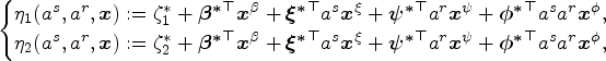
Focussing on the household ordinal outcome (2), we define the household blip function as
The optimal household decision rules:
Further, if we know the blip parameters
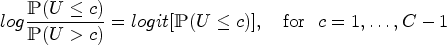
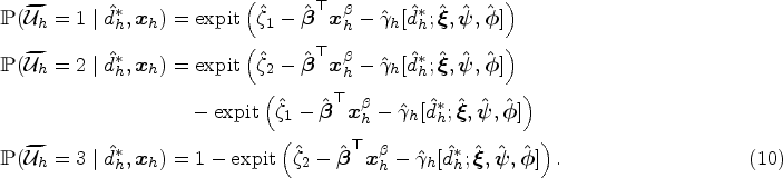
Under household interference, in a single-stage decision setting, we assume that the true ordinal-outcome model is, for


As stated in the following theorem, Step 2 in WPOM serves as the crucial key to ensuring approximate double robustness in consistently estimating the blip parameters, even when one of the treatment-free or joint propensity models is not correctly specified.
Approximate Double Robustness of WPOM: Under the identifiability assumptions of (1) consistency
18
; (2) no unmeasured confounders; and (3) positivity,
19
and suppose that the true ordinal-outcome model satisfies


Regarding the approximate double robustness of WPOM, the ‘approximate’ corresponds to ‘approximately consistent’, which refers to a case where the estimators are derived from the estimating functions which are approximately unbiased with a small quantifiable bias (see proof of Theorem 1 in Appendix A). We also use terms such as ‘nearly unbiased’ or ‘approximately unbiased’, and this quantifiable bias will be small when a linear predictor tends to vary in an interval where the
To maximize the assurance of approximate double robustness, we further present methods of estimating the joint propensity score that takes account of the correlations between treatments of individuals in the same household. 3 In a case where the treatments are correlated, the joint propensity functions are not equal to the product of the marginal propensities. To build accurate balancing weights and thus make robust estimations of optimal DTRs, we take into account the dependence among treatments observed in the same household.
To estimate the joint propensity score, letting
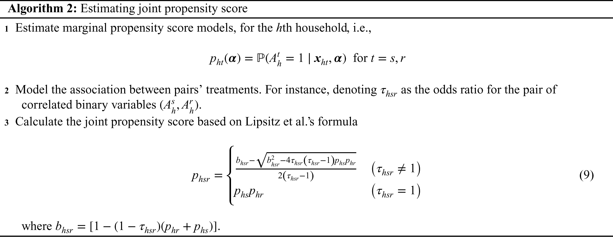
For the first step, where we estimate marginal propensity score models (
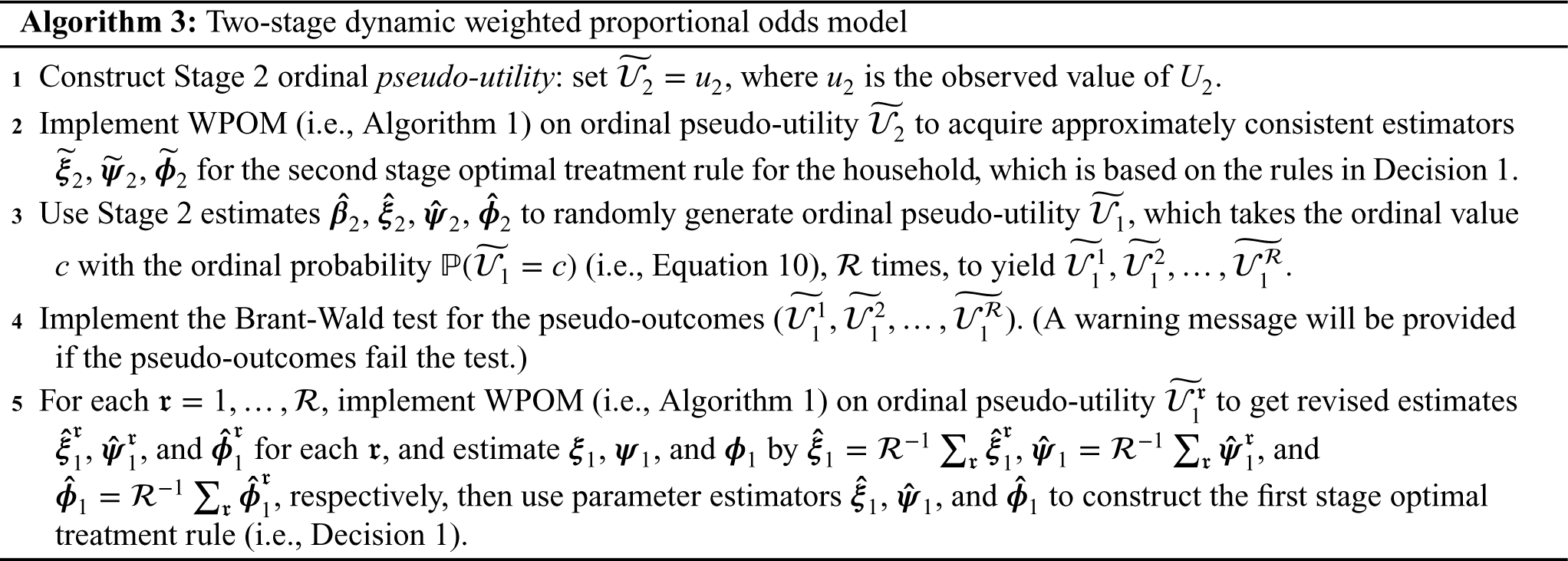
Multiple-stage decisions with household ordinal utilities
For the multi-stage treatment decision setting, backward induction is utilized in most methods for sequential decision problems. Therefore, multi-stage treatment decision problems can be broken down into a group of single-stage decision problems. Then, for each stage, we employ a WPOM to consistently estimate the blip parameters, i.e.,
If we acquire parameter estimates 
In this section, we provide two simulation studies (Study 1 and 2) to illustrate our proposed methods for estimating optimal DTRs with ordinal outcomes under household interference. In each study, we first verify the approximate double robustness of our estimation method and then check that the corresponding estimated optimal DTR outperforms those corresponding to other estimation methods. In Study 1, we consider single-stage treatment decision problems, and in Study 2, we investigate a multi-stage decision problem in a two-stage case.
To assess the performance of the methods, we construct three measures: (1) Optimal treatment rate (OTR), (2) mean regret value (MRV), and (3) value functions for ordinal outcomes. First, based on the data-generating parameters, we can calculate the truly optimal treatments for each household. Then, we can construct the recommended treatments from the estimated rules based on the estimated decision parameters. The OTR is then the percentage of the estimated recommended treatments that are in accord with the authentic optimal treatments. Second, the MRV measures the difference between the blip value under the true optimal regime and under the estimated regime and therefore measures the ‘loss’ experienced by using the estimated regime instead of the truly optimal one. The detailed performance matrix outlining the definitions of the OTR and MRV is provided in Appendix D of the Supplemental Materials (subsection 5.1). Finally, we construct value functions for ordinal outcomes, which mainly compare the estimated optimal treatments with the observed treatments. We will give the formal definition of the value functions for ordinal outcomes building on the concept of the odds ratio. It is important to note that, because of the specific nature of ordinal outcomes, for the single-stage settings in Study 1, we compare the WPOM with methods that ignore interference (Study 1a), and focus on consistent estimation of the WPOM (Study 1b). For the multi-stage settings in Study 2, we primarily concentrate on the long-term treatment effects of the estimated DTRs. In that case, we examine value functions for ordinal outcomes to compare different methods.
Single-stage treatment decision for a couples case
Single-stage treatment decision for a couples case
In Study 1a, to evaluate the performance of the proposed WPOM, we compare the proposed approach with a simpler alternative that neglects interference. Specifically, we fit a standard logistic regression model separately for husbands and wives, each with their respective treatment, covariates, and household-level covariates. An example would be the model in Theorem H.2 in Jiang,
20
which is developed without considering the treatment of the spouse. We refer to this method as an interference-unaware approach. We derive optimal treatment regimes by maximizing the conditional logistic probabilities associated with each individual and compare their performance with that of the interference-aware method. Furthermore, we have developed a cross-validation variant of WPOM by partitioning the data into
In the generation of ordinal outcomes for the households, based on the mixed cumulative logit model (2), the ordinal outcome is a random function of household treatment assignments and covariates
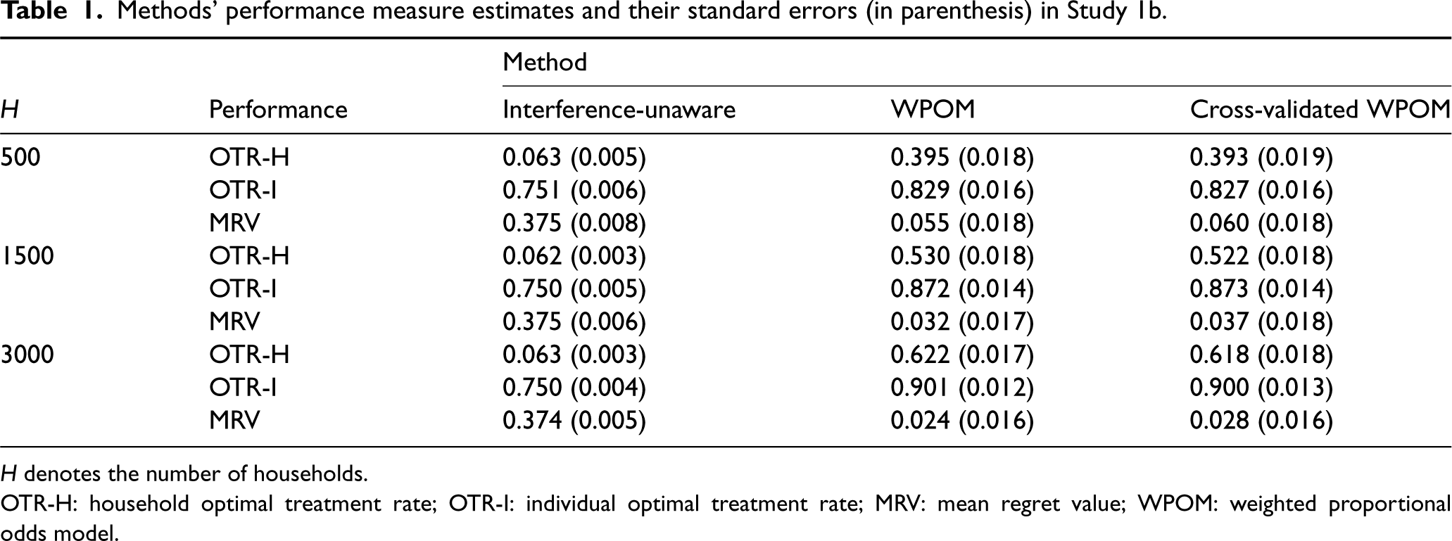
Table 1 presents the three aforementioned performance metrics for the proposed WPOM method with the weights computed based on Algorithm (2), comparing it with the interference-unaware approach and the developed
Methods’ performance measure estimates and their standard errors (in parenthesis) in Study 1b.
Methods’ performance measure estimates and their standard errors (in parenthesis) in Study 1b.
In Study 1b, to examine the approximate double robustness of the proposed method, we examine four scenarios. Scenario 1: Neither the treatment-free model nor the treatment model is correctly specified. Scenario 2: The treatment-free model is correctly specified but the treatment model is misspecified. Scenario 3: The treatment model is correctly specified but the treatment-free model is misspecified. Scenario 4: Both treatment-free model and treatment model are correctly specified.
Scenario 1 fails to specify a correct model, so consistent estimation of the blip parameters cannot be guaranteed. However, Scenarios 2, 3, and 4 correctly specify at least one of the treatment-free and treatment models, so the estimator of blip parameters should be close to consistent. In addition, note that we have only linear terms in our POM, while the true models can contain non-linear terms. If the true models contain non-linear terms, then we have misspecified the model. Moreover, in a real application, it is typically more challenging to correctly specify the treatment-free model than the treatment model, so we particularly highlight the results of Scenario 3.
In each scenario, five different methods are investigated. Method 0 (M0) employs the proposed POM (2) without any balancing weights. Method 1 (M1) considers the same POM and uses the standard balancing weights, but assumes independence between the treatments like the weights in Jiang et al.
1
That is,
Note that M0 is
The treatment decision rules in Decision 1 rely on the estimates of blip parameters, that is,
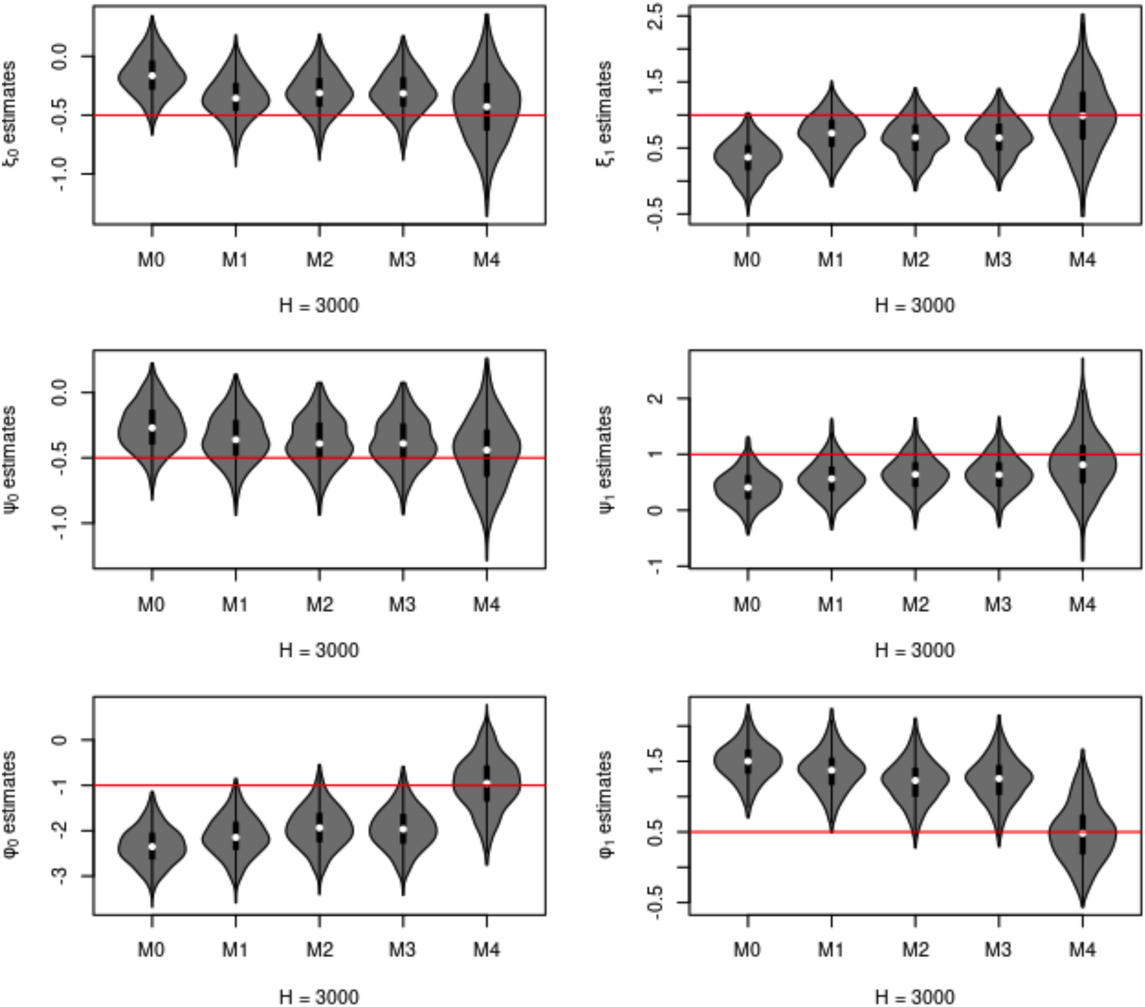
Blip function parameter estimates,
In this second part of Study 1b, focusing on Scenario 3, the settings are the same as those introduced above, except that we set different numbers of households
Simulation Study 2, a second simulation in a two-stage decision setting to demonstrate proposed dWPOM, is presented in Supplemental Materials Appendix E. These simulation results further demonstrate the robust estimation of the blip parameters resulting from the proposed method.
Data source and definition of treatments and outcome
Investigating household ordinal outcomes, we now apply our approach, dWPOM with household interference, to longitudinal survey data in the PATH study. We aim to estimate the optimal DTR for a pair in the same household, based on a sequence of rules of e-cigarette use or non-use, for achieving the smoking cessation of the pair in the household. Building on the PATH analysis in Jiang et al.,
1
we consider the subset of participant pairs both of whom smoke at the beginning of the study. In the PATH study, data were gathered in waves, starting from 2011, with each subsequent wave beginning approximately one year after the previous one. Studying the first four waves, we formulate the PATH analysis as a three-stage decision problem by defining the
In this analysis, the treatment variable is the use of e-cigarettes by cigarette smokers. Because waves were separated for approximately one year, we define e-cigarette use reported at the wave of the measured outcome as indicative of the pre-wave treatment. The e-cigarette usage variable is determined by the question ‘Do you now use e-cigarettes (a) Every day (b) Some days (c) Not at all’. Answers of either ‘Every day’ or ‘Some days’ are coded as
Further, our household ordinal utility is constructed by a combination of binary outcomes of individuals sharing a household, where the binary outcome variable is an indicator of whether participants have either given up smoking (traditional cigarettes) or have tried to quit smoking or using tobacco product(s). That is, the household utility is the sum of the final binary outcomes of a pair in the same household, which is interpreted, for a pair in a household, as (a) neither, (b) one, or (c) both of them incur a benefit such as smoking cessation. Jiang 20 provides a comprehensive discussion on the precise construction of binary outcomes using questionnaires.
Household covariates choice and model settings
As for the household covariates choice in our POM, for the
For the household covariates, we have denoted, age, education, non-Hispanic, race, and ‘plan to quit’, as the covariates
To construct the balancing weights for the proposed POM, as introduced in Section 2.4, we estimate the marginal propensity scores, the pairwise odds ratios (
Following the methods that were introduced in Section 2, we can further estimate the joint propensity score, and the corresponding weights. In particular, we compare four different weights, which are (I) no balancing weights (M0), (II) no-association overlap weights (M1), where the joint propensity functions are equal to the product of marginal propensities, (III) association-aware overlap weights (5) (M3), and (IV) adjusted association-aware overlap weights (66) (M4). In this PATH analysis, we call them Methods I (
PATH analysis results
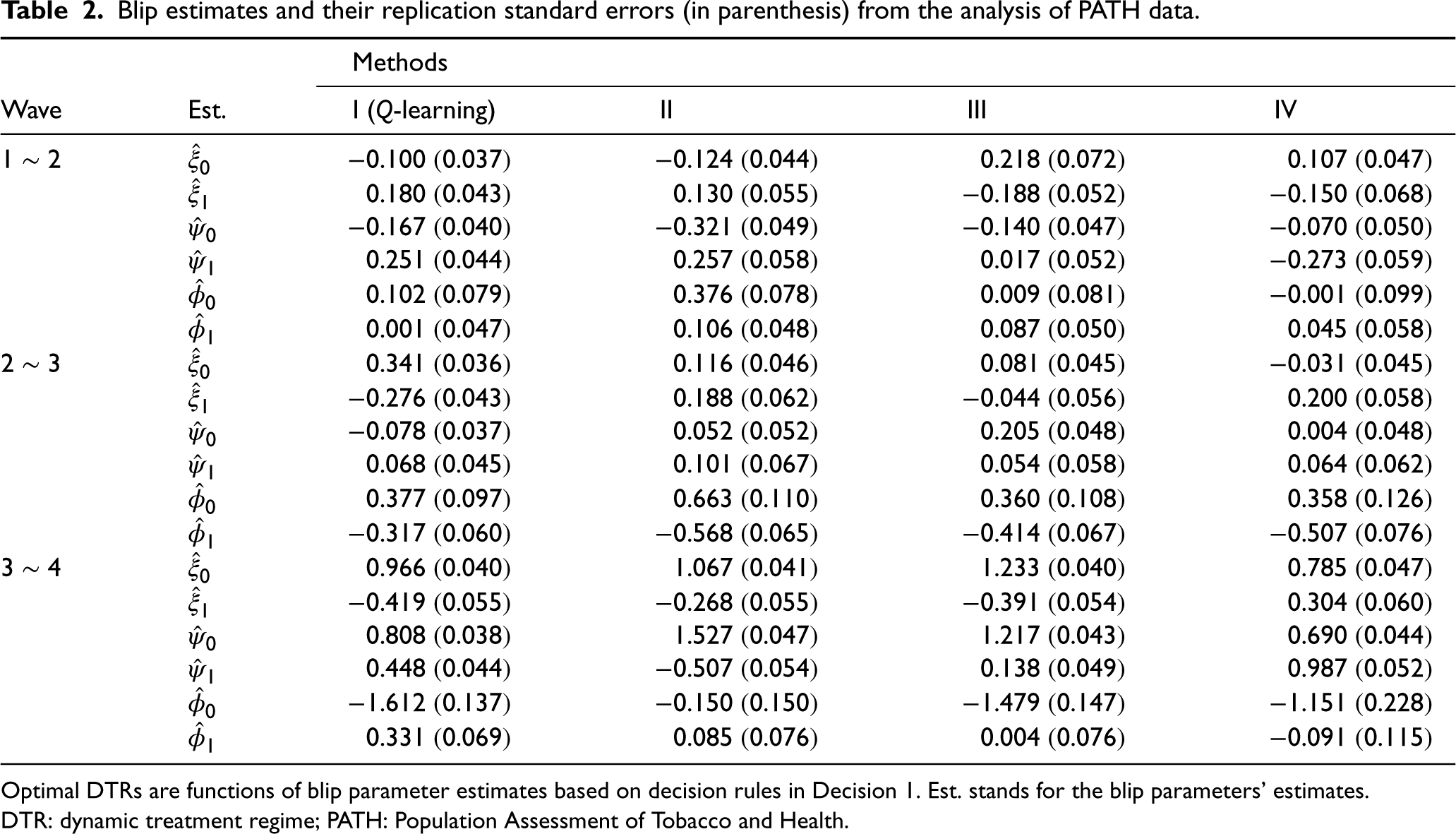
Table 2 summarizes the blip estimates and their replication standard errors (in parenthesis) from Methods I, II, III, and IV in this PATH analysis. It is important to note that, for both members of a couple to either quit or attempt to quit smoking, the optimal DTRs for the household are functions of blip parameter estimates and the couple’s tailoring variables, that is, the decision rules in Decision 1. Method IV, which employs the adjusted balancing weights, is expected to provide a consistent estimation of these blip parameters. Thus, we particularly focus on the results from Method IV, while accounting for those from other methods.
Blip estimates and their replication standard errors (in parenthesis) from the analysis of PATH data.
Blip estimates and their replication standard errors (in parenthesis) from the analysis of PATH data.
Optimal DTRs are functions of blip parameter estimates based on decision rules in Decision 1. Est. stands for the blip parameters’ estimates. DTR: dynamic treatment regime; PATH: Population Assessment of Tobacco and Health.
Because the household case with four treatment configurations is more complicated than in the previous individual-level analysis, based on Rule 1, we give several examples of how the results may be interpreted. For Method IV, in Stage 3 (Wave
Blip estimates for different treatment configurations
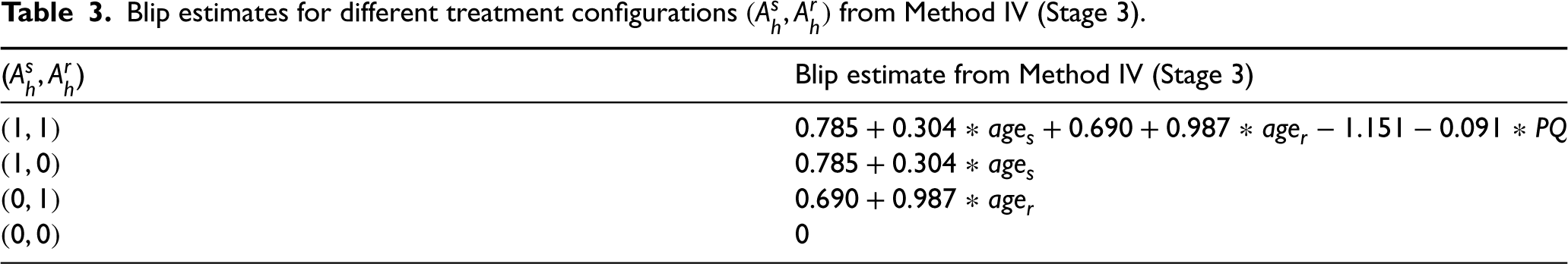
If we have household tailoring variables such that
If we have household tailoring variables such that
Finally, we note that an important aspect of rigorous real data analysis is implementing cross-validation to evaluate proposed methods properly. While the complexity of the PATH design may pose challenges, McConville, 25 Opsomer and Miller 26 and You 27 suggest that there are alternative cross-validation strategies and literature available to address these challenges, specifically in the context of complex survey data. Users should carefully choose and adapt cross-validation methods to suit their specific data and research needs, ensuring the reliability and validity of their results. Consequently, a further research direction for our methods entails an examination of suitable cross-validation strategies for analyzing data from complex longitudinal surveys.
In this paper, considering household interference and household utility, we proposed a robust DTR estimation method for ordinal outcomes to consistently estimate optimal DTRs. This method, namely dWPOM, uses sequential WPOM with adjusted balancing weights. We theoretically and empirically demonstrated the approximate double robustness property of our WPOM approach, which utilizes the proposed adjusted balancing weights. In the presence of household interference, our WPOM addresses household ordinal utility problems and provides optimal treatment recommendations for both individuals in the household. To address the ordinal outcomes challenge, we consider a POM because of its easy estimation and interpretation and note that any POM-related tools or techniques, such as those for variable selection or model diagnosis of POMs, can be employed in our method. Regarding inference, a single-stage decision can use standard errors from WPOM to create confidence intervals for blip parameters directly. However, for multi-stage decisions, non-regularity issues arise. 28 Hence, future research is needed to develop methods like adaptive bootstrap and m-out-of-n bootstrap 28 for constructing multi-stage decision confidence intervals.
We have also made a methodological contribution to the study of interference. In addition to considering the effects of neighbours’ treatments on an individual’s outcome, we considered a possible association between their treatments. Building on this, we presented the estimation process for joint propensity scores in the case where there exists an association between treatments of individuals in the same household, then estimated the corresponding balancing weights that satisfy the balancing criterion. Our simulation studies have revealed that if there exists an association between treatments but we fail to consider it, then the DTR estimation process will lead to bias. It would be straightforward to extend our household interference case to cases of partial interference, where treatments of individuals blocked by clusters can affect outcomes of the individuals in the same cluster, while also accounting for the association between these treatments of individuals in the same cluster. However, the association-aware estimation has an extra cost: Modelling association between pairs of binary treatments, such as through a pairwise odds ratio model in our household case. For the cluster partial-interference case, we suggest considering the log-linear model to extend our work to estimate the ‘higher-order’ odds ratio association. 29 Note that in cases of association, the final goal is to estimate the joint propensity scores; therefore, we recommend employing machine learning methods, such as random forest or deep neural network, to directly train the model for the joint propensity scores.
We acknowledge that any misspecification in the association model (Step 2 of the Algorithm 2) could impact the accuracy of our joint propensity score estimation, and thus affect the approximate double robustness of the proposed method. This step could be refined by using flexible data-adaptive approaches that accommodate correlated data. Examples of such approaches include mixed-effect machine learning 30 and smoothed kernel regression designed for dependent data. 31 Further investigation is needed to assess the robustness of the proposed methods in terms of association models and employing these data-driven approaches. Our formulation through the household utility function also allows for some association among the responses of the household members, conditional on their treatments. In particular, when we define household utility as a function of the sum of individual utilities, which happens to be the sum of their response indicators, the utility distribution will imply an association between the responses of paired members.
We also note that individuals within the same household may experience varying magnitudes of interference effects. When the objective is to optimize the household’s utility function, the fourth term in our model (Equation 1) captures these interference effects, and distinguishing between the effects on individuals may not be necessary. However, if the goal is to optimize individual outcomes or understand the role of interference effects for each person (e.g., husband or wife), distinguishing between these interference effects becomes essential. To achieve this, we can examine individual outcome models, which involve modelling the outcomes of the husband and wife separately, such as using distinct logistic regression models. For a consistent estimation approach in logistic regression, we refer to Appendix H.1.2 in Jiang, 20 where the balancing property with household interference for binary outcomes was proposed for generalized linear models that consider interference. It would be of interest to explore further the estimation and development of optimal decision rules for this approach, in order to compare it with the approach based on household outcomes.
Extending the proposed method to households with varying numbers of individuals, including those with more than two individuals, presents a challenging yet important endeavour. This extension can be likened to addressing a partial interference32,4 problem, where treatments of individuals blocked by clusters can affect outcomes of the individuals in the same cluster, and households can be viewed as distinct clusters. To address the partial interference problem, two modelling are necessary for the investigation: (1) modelling the outcomes, this entails developing regression models for the outcomes. It is worth noting that dealing with high dimensionality (e.g., the treatment indicators of all study units in the cluster and cluster-level pre-treatment covariates) may necessitate additional assumptions, such as conditional stratified interference, to mitigate the challenges posed by the curse of dimensionality; see Section 2.2 of Park et al. 4 for additional discussions about these assumptions; (2) modelling the joint propensity scores: In the context of the joint propensity scores, it’s important to consider the potential removal of the treatment-independent assumption as we investigated in Section 2.4. This can be achieved by accounting for the associations between treatments of individuals within the same cluster.
Through our analysis of the PATH study, we have demonstrated the practical applicability of our proposed methods. We estimated a treatment decision function for household pairs to maximize the probability of achieving smoking cessation under the assumptions of a model for their treatment and success. In particular, we modelled the potential association of e-cigarette usage between members of a household pair and estimated the joint propensity scores that play a crucial role in approximately doubly robust estimation with interference. We acknowledge some limitations of our analysis: the PATH data points are a year apart, which is not an ideal spacing for treatment decisions, and the size and period of the PATH subsample provide insufficient data on some of the possible treatment sequences to make the findings easily interpretable or conclusive. In addition, we have implicitly assumed that there is meaning in having been the first of the two household members to be interviewed. While this could well be the case in practice (e.g., the household head is interviewed first), it is important to recognize the semi-arbitrary nature of this labelling, and to assess its impact in future research. Due to these limitations, it is essential to note that the results of our PATH analysis are not intended as authentic treatment recommendations for smoking cessation. They nonetheless serve to demonstrate the underlying principles of household interference in such a context and the methodology we propose in this analysis.
Supplemental Material
sj-pdf-1-smm-10.1177_09622802241242313 - Supplemental material for Estimating dynamic treatment regimes for ordinal outcomes with household interference: Application in household smoking cessation
Supplemental material, sj-pdf-1-smm-10.1177_09622802241242313 for Estimating dynamic treatment regimes for ordinal outcomes with household interference: Application in household smoking cessation by Cong Jiang, Mary Thompson and Michael Wallace in Statistical Methods in Medical Research
Supplemental Material
sj-zip-2-smm-10.1177_09622802241242313 - Supplemental material for Estimating dynamic treatment regimes for ordinal outcomes with household interference: Application in household smoking cessation
Supplemental material, sj-zip-2-smm-10.1177_09622802241242313 for Estimating dynamic treatment regimes for ordinal outcomes with household interference: Application in household smoking cessation by Cong Jiang, Mary Thompson and Michael Wallace in Statistical Methods in Medical Research
Footnotes
Data availability
The data that support the findings of this study come from the PATH Study. Restrictions apply to the availability of these data, which were used under license for this study. Data collected in the PATH Study are available from ![]() with the permission of the Population Assessment of Tobacco and Health Study Restricted-Use Files (ICPSR 36231).
with the permission of the Population Assessment of Tobacco and Health Study Restricted-Use Files (ICPSR 36231).
Declaration of conflicting interests
The authors declared no potential conflicts of interest with respect to the research, authorship, and/or publication of this article.
Funding
The authors disclosed receipt of the following financial support for the research, authorship, and/or publication of this article: This work has been supported by the Ontario Institute for Cancer Research (OICR) Biostatistics Training Initiative (BTI) Studentship Award through funding provided by the Government of Ontario, by funds from a CIHR Project Grant to M. P. Wallace, and by a Discovery Grant to M. E. Thompson (RGPIN-2016-03688) from NSERC.
Supplemental material
Additional supporting information can be found online in the Supporting Information section.
References
Supplementary Material
Please find the following supplemental material available below.
For Open Access articles published under a Creative Commons License, all supplemental material carries the same license as the article it is associated with.
For non-Open Access articles published, all supplemental material carries a non-exclusive license, and permission requests for re-use of supplemental material or any part of supplemental material shall be sent directly to the copyright owner as specified in the copyright notice associated with the article.