Sage Journals: Discover world-class research

Abstract

Joint modelling of longitudinal and time-to-event data is a method that recognizes the dependency between the two data types, and combines the two outcomes into a single model, which leads to more precise estimates. These models are applicable when individuals are followed over a period of time, generally to monitor the progression of a disease or a medical condition, and also when longitudinal covariates are available. Medical cost datasets are often also available in longitudinal scenarios, but these datasets usually arise from a complex sampling design rather than simple random sampling and such complex sampling design needs to be accounted for in the statistical analysis. Ignoring the sampling mechanism can lead to misleading conclusions. This article proposes a novel approach to the joint modelling of complex data by combining survey calibration with standard joint modelling. This is achieved by incorporating a new set of equations to calibrate the sampling weights for the survival model in a joint model setting. The proposed method is applied to data on anti-dementia medication costs and mortality in people with diagnosed dementia in New Zealand.

Keywords

Calibration survival analysis sampling weights longitudinal models cost analysis

1. Introduction

Joint modelling of longitudinal and time-to-event data allows simultaneous modelling of a longitudinal variable and time-to-event process, by using sub-models to model each data type within a single model.¹ Joint models are useful when dealing with survival models with measurement error, partially missing time-dependent covariates, longitudinal models with informative dropouts, or survival process and longitudinal process that are associated via latent variables.² These models reduce bias in parameter estimates within a single study, which makes joint models useful and preferable to performing longitudinal or time-to-event analyses separately.¹ Slasor and Laird³ demonstrated efficiency gains of 6.4% and 10.2% when using the joint piece-wise exponential joint model over the standard proportional hazards model in a simulation and clinical trial data, respectively.

Longitudinal data is composed of continuous or discrete repeated measures from particular individuals followed over a period of time. This sort of data is particularly useful for evaluating the relationship between risk factors and development of a disease, and the outcomes of treatments over time.⁴ Time-to-event data records the length of time until the occurrence of a well-defined end-point of interest and is widely used in many statistical techniques such as Cox proportional hazards models.⁵ Joint models allow us to deal with these two data types simultaneously by considering the dependency between them, using submodels that depend on each other. These models are applicable when individuals are followed over time, generally to observe the progression of a disease or a medical condition or death, and when longitudinal variables that are related to the time-to-event variable, such as monthly medical costs, are available.

Joint models are important as they provide more efficient estimates of the effects on the time-to-event variable, provide more efficient estimates of the effects of the longitudinal variables, and reduce bias in the estimates of the overall effects, that is, the effect on survival and the longitudinal variable.⁶ One of the possible strategies that can be used in the joint modelling of longitudinal and survival data is to incorporate the longitudinal measurements directly into the Cox model as time-dependent covariates to perform Cox model analysis. However, because the longitudinal measurements are typically correlated between the same subject, this approach might lead to highly biased and inefficient estimates of the treatment effect. Tsiatis et al.⁷ proposed the two-stage approach, in which a linear mixed model is fitted to the longitudinal data in the first stage and the fitted trajectory function is incorporated into the Cox model as a time-dependent covariate in the second stage but this approach still leads to potentially biased estimates.⁶ Instead of using this approach, joint modelling of longitudinal and survival data can effectively remove this bias, by using individual-level random effects that account for both the association between the longitudinal and time-to-event outcomes, and the correlation between the longitudinal measurements in the longitudinal sub-model.⁸ Therefore, joint models should be used as they do not lead to biased estimators.

Another challenge is that due to the increasing availability of electronic health records, increasingly more health services research questions are answered using secondary analysis of such national data sets, which are often obtained using complex sampling designs. Ignoring this design can result in severely biased estimates.⁹ Therefore, the sampling design must be taken into account in the analysis. In complex samples, subjects are selected using sampling designs in which some subjects have higher or lower selection probabilities. Sampling weights are defined as the inverse of the selection probabilities. The weights can be interpreted as the number of individuals each individual represents in the population. These weights are used to multiply the log-likelihood contribution from each subject, accounting for the sampling design.

This article extends the pseudolikelihood approach to calibrated weights. The weights are calibrated to surrogates of the survival model influence functions. This is done by incorporating a new set of equations that calibrate the sampling weights. We use a two-phase design approach which has been previously used.¹⁰ Our approach using weights calibrated to surrogates of the survival model influence functions results in more efficient estimates of the survival model parameters for variables that are available for the whole population.

2. Two-phase designs

In two-phase designs,¹¹ the first-phase sample (population) of size $N$ is assumed random, and the second-phase sample of size $n$ is selected from the first phase, based on information available at the first phase. For example, the second-phase sample can be a stratified sample, or an outcome dependent sample.^12,13 Generally, inexpensive information is available at the first phase, and expensive covariates are collected in the second phase sample. The two-phase design is advantageous when it is expensive to collect exposure variables on all subjects.¹³ This is a superpopulation approach in order to be able to combine sampling techniques with modelling approaches.¹⁴ While minimizing the cost of collecting data for every subject, the purpose of two-phase sampling is to fit the model of interest using the phase-two sample and obtain results that would have been gained by fitting the same model using the phase-one data.¹² Two-phase samples can also arise from a missing data mechanism or complex sampling designs.

3. Joint model of medical cost and mortality

A joint model of medical cost and survival can be a single model consisting of two or three sub-models. For example, assume a group of $N$ individuals whose medical costs are observed longitudinally. The costs of the individual $i$ , available for phase-one sample of size $N$ , are denoted by $y_{i} = (y_{i 1}, y_{i 2}, \dots, y_{i, N_{i}}$ ), where $y_{i j}$ is the cost for individual $i$ at time $j$ where $j$ = 1, 2,…, $N_{i}$ , and $N_{i}$ is the number of repeated measurements available for individual $i$ in the phase-one sample. Let $t_{i}$ = min( $c_{i}$ , $d_{i}$ ) be the observed follow-up time, where $c_{i}$ is the censoring time independent of the cost and $d_{i}$ the time of death. A death indicator is denoted as $Δ_{i}$ = $I$ ( $d_{i}$ $\leq$ $c_{i})$ and $x$ is the vector of covariates available only for the phase-two sample of size $n$ and $z$ is the vector of auxiliary variables available for phase-one sample. $x$ is split into $x_{1_{i j}}$ and $x_{2_{i}}$ , where the former is a longitudinal variable for the cost models to model longitudinal medical cost where $x_{1_{i}} = (x_{i 1}, x_{i 2}, \dots, x_{i, n_{i}})$ with $n_{i}$ being the number of repeated measurements available for individual $i$ in the phase-two sample, and the latter is an individual-level variable in the survival model. Similarly, $z$ is split into $z_{1_{i}}$ and $z_{2_{i}}$ where the former is a longitudinal auxiliary variable for the cost model and the latter is an individual-level auxiliary variable in the survival model.

Xu et al.⁹ used the approach proposed by Liu et al.¹⁵ to jointly model the cost $y_{i j}$ and time-to-event, but using the flexible generalized gamma distribution with parameters $κ$ , $μ_{i j}$ and $σ_{i j}$ instead of using the log-normal distribution. We use the gamma distribution with shape parameter $σ^{2}$ and scale parameter $\frac{μ_{i j}}{σ^{2}}$ to model the positive monthly medical cost. The resulting joint model is defined as

\begin{aligned} η_{i j} = {x_{1_{i j}}}^{T} α_{1} + {z_{1_{i j}}}^{T} α_{2} + a_{i} \\ μ_{i j} = \exp ({x_{1_{i j}}}^{T} β_{1} + {z_{1_{i j}}}^{T} β_{2} + λ_{1} a_{i} + b_{i}) \\ σ_{i j}^{2} = \exp (δ) \\ h_{i} (t) = h_{0} (t) \exp ({x_{2_{i}}}^{T} γ_{1} + {z_{2_{i}}}^{T} γ_{2} + λ_{2} a_{i} + λ_{3} b_{i}) \end{aligned}

(1) where

α, β, γ, λ_{1}, λ_{2} and λ_{3}

are unknown parameters of interest. Note that there are three sub-models. The first sub-model,

η_{i j}

is defined as logit(

P (y_{i j} > 0 | x_{i j}, a_{i}, α

)), and models the probability of incurring a positive medical cost (i.e., having a prescription). The second sub-model

μ_{i j}

models the amount of positive model cost, and the third sub-model,

h_{i} (t)

, is the survival sub-model to model survival, where

h_{0} (t)

is the baseline hazard function for the time-to-event outcome. There are two individual-specific random effects,

a_{i} \sim N (0, σ_{a}^{2})

and

b_{i} \sim N (0, σ_{b}^{2})

, which are assumed to be independent of each other. The random effects are incorporated to account for variability between individuals in each sub-model. These random effects are shared across the sub-models

η_{i j}

μ_{i j}

and

h_{i} (t)

to correlate the probability of having positive costs, the positive medical cost and the survival. The dispersion parameter

σ_{i j}

allows heteroscedasticity to be modelled using covariates.

4. Parameter estimation

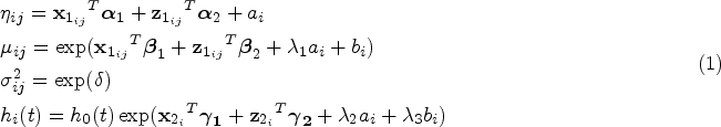
For a single individual $i$ , the likelihood contribution is given by

\begin{aligned} L_{i} (θ) = \iint \exp (l_{i}^{A}) \exp (l_{i}^{B}) \exp (l_{i}^{C}) f (a_{i}) f (b_{i}) d a_{i} d b_{i} where \\ l_{i}^{A} = \sum_{j = 1}^{n_{i}} [I_{i j} \log (η_{i j}) - \log (1 + \exp (η_{i j}))] \\ l_{i}^{B} = \sum_{j = 1}^{n_{i}} I_{i j} [- \frac{μ_{i j}}{σ^{2}} \log (σ^{2}) - \log Γ (\frac{μ_{i j}}{σ^{2}}) + (\frac{μ_{i j}}{σ^{2}} - 1) \log (y_{i j}) - \frac{y_{i j}}{σ^{2}}] \\ l_{i}^{C} = Δ_{i} (\log h_{0} (t_{i}) + {x_{2_{i}}}^{T} γ_{1} + {z_{2_{i}}}^{T} γ_{2} + λ_{2} a_{i} + λ_{3} b_{i}) \\ - \int_{0}^{t_{i}} h_{0} (s) \exp ({x_{2_{i}}}^{T} γ_{1} + {z_{2_{i}}}^{T} γ_{2} + λ_{2} a_{i} + λ_{3} b_{i}) d s \end{aligned}

where

θ

is the vector of all unknown parameters of interest including

α, β, γ, λ_{1}, λ_{2}, λ_{3}, σ_{a} and σ_{b};

f (a_{i})

and

f (b_{i})

are the density functions for the random effects

a_{i}

and

b_{i}

;

l_{i}^{A}

l_{i}^{B}

and

l_{i}^{C}

are the log-likelihood contribution of each of the sub-models. Note that

l_{i}^{A}

models the probability of having a positive medical cost,

l_{i}^{B}

, is from a gamma distribution with shape parameter

σ^{2}

and scale parameter

\frac{μ_{i j}}{σ^{2}}

, modelling the positive monthly medical cost and

l_{i}^{C}

models the survival. If we assume the data were collected using a simple random sampling (SRS) design, then the joint likelihood of all individuals is given by

L (θ) = \prod_{i = 1}^{n} \iint \exp (l_{i}^{A}) \exp (l_{i}^{B}) \exp (l_{i}^{C}) f (a_{i}) f (b_{i}) d a_{i} d b_{i}

(2) which is a multiplication of all individual likelihoods. In the joint modelling of longitudinal and survival data, the main interest may be on modelling survival data or longitudinal data, or it can be of both types of data.¹⁶ Our focus is modelling both outcomes. The log-likelihood is given by

l (θ) = \sum_{i = 1}^{n} \log L_{i} (θ)

(3) In complex samples where certain subsets of the population are oversampled, the sample is informative, but it is not directly representative of the population.¹⁷ Ignoring this in the analysis can lead to biased estimates where standard errors may be underestimated resulting in misleading conclusions.¹⁸ It is therefore important to account for sampling weights and design effects in the statistical analysis.¹⁹

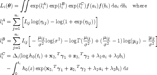
Recent literature in joint modelling has been based on the assumption that the data set was obtained via a SRS design, despite the fact that samples obtained from health records are usually complex.⁹ To allow for the fact that data is collected using a complex sampling design, Xu et al. proposed an approach to incorporate sampling weights into the log-likelihoods.

4.1. Pseudolikelihood

To recognize the complex survey setting of the data, sampling weights $w_{i}$ , need to be incorporated into equation (3) to obtain unbiased parameter estimates. Assuming that sampling is at the individual-level, the log-likelihood contribution from individual $i$ is multiplied by its corresponding sampling weight to form the log-pseudolikelihood

l_{w} (θ) = \sum_{i = 1}^{n} w_{i} \log L_{i} (θ)

(4) That is, the sampling weights multiply the corresponding subject log-likelihood contribution in (3), which leads to the log-pseudolikelihood in equation (4). The integrals in (2) can be solved using the Gaussian quadrature or Laplace approximation. Since these techniques cannot be directly applied to the unspecified non-parametric baseline hazard

h_{0} (t)

, the hazard is first replaced with a piece-wise constant function. To implement this, we follow the approach by Xu et al. We divide the follow-up period into

K

intervals by using quantiles of survival times, where the baseline hazard is now assumed to be the constant on each of the intervals, such that

{\tilde{h}}_{0} (t) = h_{0 k}, t \in (Q_{k - 1}, Q_{k}]

(5) where

k = 1, 2, \dots, K

and

Q_{k}

= (100

k

K

)th quantile of all survival times with

Q_{0}

= 0. This is the standard approach followed in the Cox model literature to profile out the likelihood.²⁰ When we use

{\tilde{h}}_{0} (t)

instead of

h_{0} (t)

, the likelihood becomes parametric, enabling Gaussian quadrature or Laplace approximation to be applied. Once the parametric

\tilde{h_{0}} (t)

is used in place of the non-parametric baseline hazard

h_{0} (t)

, the set of unknown parameters of interest

θ

can be estimated.

4.2. Calibrated pseudolikelihood

Deville and Särndal²¹ proposed the theory of survey calibration (generalized raking), which uses calibrated weights to improve efficiency of estimators of totals from complex surveys, in cases where auxiliary variables for which the population total is known are available. The goal is to improve estimators of the form

{\hat{t}}_{x π} = \sum_{s} w_{i} x_{i}

(6) where

w_{i}

is the inverse of the strictly positive inclusion probability of individual

i

in the population and

x

is a variable of interest. Survey calibration aims to obtain

{\hat{t}}_{x w}

\sum_{s} w_{i}^{'} x_{i}

, a new estimator that has the modified weights

w_{i}^{'}

which ensures that the total of the auxiliary variable

z_{i}

is perfectly estimated. To obtain

w^{'}

, a distance between the two weights,

w_{i}

and

w_{i}^{'}

is minimized subject to the calibration constraint given by

t_{z} = \sum_{s} w_{i}^{'} z_{i}

(7) which is the exact estimator of population total for

z_{i}

, which is assumed to be accurately known. There are various distance functions including raking calibration which uses distance functions that always returns positive calibrated weights.²¹

4.3. Surrogates of the influence functions

Calibration performs well when estimating totals, and the auxiliary variables are strongly correlated with the study variable of interest.²¹ Our parameter estimator is not a total, but we can express it asymptotically as total, with the help of influence functions (IFs) given by

\sqrt{N} (\hat{γ} - γ) = \frac{1}{\sqrt{N}} \sum_{i = 1}^{N} {h}_{i} (γ) + O_{p} (1)

(8) where

h_{i} (γ)

is the IF for the

i

th individual. This approach has been used before to gain efficiency when estimating parameters in other models.^10,22,23,24

The dfbeta’s can be used as precise approximations of the IFs,²⁵ where dfbeta for individual $i$ is defined as the difference between the estimator based on the sample of size $N$ and the estimator gained when individual $i$ is excluded. Kulich and Lin²⁶ used an imputation for the partially missing variables using the prediction model fitted on the phase-two sample. This approach makes it possible to estimate the influence functions using the imputations of the partially missing variables and the phase-one data and it is likely to be most useful when the number of partially missing variables is one or two.¹⁰ This specific calibration methodology follows Breslows et al. but has been modified to meet the joint model setting, where we are using surrogates of the influence functions. We call them ’surrogates’ because they are estimated, and motivated by Breslow et al., we assume that they have an approximate linear relationship as in equation (8).

Use weighted regression models such as linear or logistic regression models to the phase-two sample, to predict the partially missing variables using variables known for all subjects. A separate prediction is required for each of the partially missing variables.

Impute the partially missing variables for every subject at phase-one, using the prediction equation obtained.

Fit a proportional hazards model to the phase-one data using the imputed values of partially missing variables. For individuals in the phase-two sample, the imputed values are used to ensure surrogates of the influence functions only depend on information available at phase-one. After the model is fitted, surrogates of the influence functions are obtained as dfbeta’s using the coxph function in R.

Calibrate the sampling weights using surrogates of the influence functions from the survival sub-model for the phase-two sample as auxiliary variables and zeroes as totals. We use raking calibration to guarantee positive adjusted weights.

Obtain parameter estimates using log-pseudolikelihood with the resulting calibrated weights. That is, solving the equations:

l_{w} (θ) = \sum_{i = 1}^{n} w_{i, C}^{'} \log L_{i} (θ)

(9) where

w_{i, C}^{'}

is the sampling weight calibrated to the surrogates of the influence functions from the survival sub-model, for the

i

th individual. The survey packagein R is used to fit the weighted prediction model and calibrate the sampling weights.²⁷

5. Variance estimation

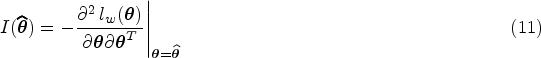
Variance is estimated differently depending on the type of estimating equations used for parameter estimation. For unweighted log-likelihood, the variance is conveniently estimated with the usual negative Hessian matrix evaluated at the parameter estimates. For log-pseudolikelihood with sampling weights, we use a sandwich estimator, obtained from Taylor linearization:

\hat{V} (\hat{θ}) = I (\hat{θ})^{- 1} G I (\hat{θ})^{- 1}

(10) where

I (\hat{θ}) = - \frac{\partial^{2} l_{w} (θ)}{\partial θ \partial θ^{T}} |_{θ = \hat{θ}}

(11) and matrix

G

G = \hat{V} (\frac{\partial l_{w} (θ)}{\partial θ}) = \hat{V} (U_{w} (\hat{θ}))

(12) the estimated variance of the score vector. To calculate

G

, assuming that the sampling design is stratified and clustered with

H

strata (

H = 1

for no stratification), the matrix

G

is given by

G = \sum_{h = 1}^{H} \frac{n_{h}}{n_{h} - 1} \sum_{l = 1}^{n_{h}} (e_{h l \cdot} - {\bar{e}}_{h \cdot \cdot})^{T} (e_{h l \cdot} - {\bar{e}}_{h \cdot \cdot})

(13) where

n_{h}

is the number of clusters in stratum

h

and

e_{h l \cdot} = \sum_{i} w_{i} \frac{\partial \log L_{i} (θ)}{\partial θ} |_{θ = \hat{θ}}

(14) and

{\bar{e}}_{h \cdot \cdot} = \frac{1}{n_{h}} \sum_{l} e_{h l \cdot}

(15) where

e_{h l \cdot}

is the sum of all individual gradient functions in stratum

h

and cluster

l

, evaluated at the maximum likelihood estimate. The sum

e_{h l \cdot}

is calculated over all individuals in stratum

h

and cluster

l

, and that for

{\bar{e}}_{h \cdot \cdot}

is calculated over all clusters in stratum

h

. For calibrated pseudolikelihood, variance can be obtained in a similar way using the calibrated weights and influence functions. Modifying (12) to account for calibration gives

I (\hat{θ})^{- 1} \hat{V} (U_{w_{C}^{'}} (\hat{θ}) - U_{w_{C}^{'}}^{'} (\hat{θ})) I (\hat{θ})^{- 1}

(16) where

U_{w_{C}^{'}}^{'} (\hat{θ}) = \sum_{i = 1} U_{w_{i, C}^{'}}^{'} (\hat{θ})

and

U_{w_{i, C}^{'}}^{'} (\hat{θ})

is the estimated score which can be obtained by regressing the scores on surrogates of the influence functions and using the fitted model to predict the score. The estimated scores can be obtained using lm function in R, with

U_{w_{C}^{'}} (\hat{θ})

as the response variable and surrogates of the influence functions as explanatory variables. Using resid function on the fitted linear regression model allows extraction of the residuals

U_{w_{C}^{'}} (\hat{θ}) - U_{w_{C}^{'}}^{'} (\hat{θ})

which replace

U_{w_{C}} (\hat{θ})

used for estimating the variance for the pseudolikelihood case.

6. Simulation study

We conducted a simulation study to investigate the efficiency of the proposed estimators. This specific setting follows Xu et al., where phase 1 is used to generate values of a phase-one sample (finite population) from the joint model and phase 2 is used to select a phase-two sample from the phase-one sample. Automatic differentiation and Laplace approximation from the TMB package²⁸ in R was used to optimize the joint likelihood and obtain parameter estimates, with log-likelihood functions coded in C++. This code is available from https://github.com/yoonsh94/joint_model.

At phase 1, the joint model used to generate the phase-one data set is given by

\begin{aligned} η_{i j} & = α_{0} + X_{1_{i j}} α_{1} + Z_{1_{i j}} α_{2} + Z_{2_{i j}} α_{3} + Z_{3_{i}} α_{4} + a_{i} \\ μ_{i j} & = \exp (β_{0} + X_{1_{i j}} β_{1} + Z_{1_{i j}} β_{2} + Z_{2_{i j}} β_{3} + Z_{3_{i}} β_{4} + λ_{1} a_{i} + b_{i}) \\ h_{i} (t) & = h_{0} (t) \exp (X_{2_{i}} γ_{1} + Z_{3_{i}} γ_{2} + Z_{4_{i}} γ_{3} + λ_{2} a_{i} + λ_{3} b_{i}) \end{aligned}

(17) where

X

variables are assumed to be available only for the phase-two sample, and

Z

variables are available for the phase-one sample. That is,

Z

variables are auxiliary variables that are used to impute

X

variables. In addition, extra auxiliary variables

(A_{1}, A_{2}, A_{3})

, which have correlations of about 0.9 with

X_{2_{i}}

, are used to fit the prediction model for

X_{2_{i}}

to provide additional information. The longitudinal covariate

X_{1, i j}

is simulated from a Bernoulli distribution with success probability 0.5,

Z_{1, i j} \sim N (X_{1, i j}, 1.5)

and

Z_{2, i j} \sim N (X_{1, i j}, 0.8)

. The number of repeated measurements available for each individual follows a poisson distribution with rate 20. The covariate

X_{2, i}

is simulated from a Bernoulli distribution with success probability 0.4,

Z_{3, i} \sim N (X_{2, i}, 1.5)

and

Z_{4, i} \sim N (X_{2, i}, 0.8)

. All covariates in the survival model are individual-level, and

Z_{3_{i}}

is an individual-level variable shared across all submodels.

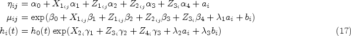
The fixed effect coefficients are set to $(α_{0}, α_{1}, α_{2}, α_{3}, α_{4})^{T}$ = $(2.5, 1, 1, 1, 1)^{T}$ , $(β_{0}, β_{1}, β_{2}, β_{3}, β_{4})^{T}$ = $(2, 1, 1, 1, 1)^{T}$ and $(γ_{1}, γ_{2}, γ_{3})^{T}$ = $(0.5, 0.5, 0.5)^{T}$ . The shared random effects are $a_{i} \sim N (0, σ_{a}^{2})$ and $b_{i} \sim N (0, σ_{b}^{2})$ , where $σ_{a}^{2} = σ_{b}^{2} = 1$ and the association parameters $(λ_{1}, λ_{2}, λ_{3})^{T}$ = $(0.7, 0.5, 0.5)^{T}$ . The positive costs are generated using the gamma distribution with shape parameter $σ^{2} = \exp (δ)$ where $δ = 0.5$ , and scale parameter $σ^{2} / μ_{i j}$ . The non-parametric baseline hazard is replaced with a piecewise constant function as discussed in (5), with $K = 10$ intervals by using quantiles of survival times. Survival times are generated using the hazard function $h_{i} (t)$ and is censored when it occurs after the censoring times, which follows an exponential distribution with rate 2. The resulting phase-one sample is of size $N = 2000$ with 10 strata, where each stratum consists of four clusters and each cluster has 50 individuals.

At phase 2, the phase-two sample is selected from the phase-one sample using a stratified cluster sampling design. Firstly, a simple random sample of two clusters is selected from each stratum. Then, individuals in each sampled cluster are selected by sampling with probability proportional to size (PPS) where the size measure is given by

\begin{aligned} S_{i} = \frac{(0.25 + 0.5 | {\bar{Z}}_{i} |) (0.5)}{1 + ϕ_{1} \exp (- 0.001 {\bar{y}}_{i})} \end{aligned}

(18)

\begin{aligned} (i) ϕ_{1} = 0 \end{aligned}

(19)

\begin{aligned} (ii) ϕ_{1} = 1 \end{aligned}

(20) Equation (19) is non-informative sampling scheme that depends only on

Z

, where

{\bar{Z}}_{i}

is the absolute average value of the covariates

Z_{1}, Z_{2}

and

Z_{3}

in the cost sub-models that are available for the phase-one sample, for individual

i

. That is, the selection probability is not associated with either the positive cost or the survival, but individuals with higher values of

{\bar{Z}}_{i}

are oversampled. Additionally, (20) is an outcome-dependent sampling scheme, in which individuals with a higher average medical cost are more likely to be included in the phase-two sample. Finally, a phase-two sample of size

n

= 200 individuals is selected. The sampling weights are computed as the inverse of the sampling probabilities and approximately sum to the phase-one sample size, and are used in equation (4) to obtain a log-pseudolikelihood expression for the individuals in the phase-two sample.

6.1. Estimated sampling weights

In practice, true sampling weights may not always be available. Alternatively, Robins et al.²⁹ suggested using estimated sampling weights using a logistic regression model, as such estimated weights lead to efficiency gains even when the true sampling weights are available. We evaluate the performance of log-pseudolikelihood (IPW) and calibrated log-pseudolikelihood estimator using estimated sampling weights in place of true sampling weights. To estimate the sampling weights using logistic regression, information about all individuals in the phase-one sample is needed.

We conduct simulation studies using two sampling schemes based on estimated sampling weights in place of true sampling weights. While the phase-one data generation process is identical to the one previously used, phase-one variables $Z_{3}$ and $Z_{4}$ are generated differently, using a Bernoulli distribution where success probability $p$ is set to be dependent on the values of $X_{2}$ , such that the correlation between $X_{2}$ and $(Z_{3}, Z_{4})$ is about 0.7 and 0.8, respectively, for calibration purposes. There are no extra auxiliary variables are involved, which closely mirrors the setting in our application data.

In the first scheme given by (21), the phase-two sample selection process is correctly accounted for by our weight estimation model. In the second scheme given by (22), the phase-two selection sample process is incorrectly accounted for by the weight estimation model, and the selection process involves an unmeasured phase-one variable ‘frailty’, which has a reasonably high bearing on phase-two sample selection, along with other known variables. The frailty variable is simulated from Bernoulli with $p$ that takes value 1 with p = 0.9 when $Z_{3}$ or $Z_{4}$ is 1. In both schemes, the phase-two sample is selected using PPS design, where phase-one individuals with larger values of certain variables are more likely to be selected in the phase-two sample.

We use $Z_{3, i}$ (i.e. gender) and $Z_{4, i}$ (i.e. age) as auxiliary variables and use these to impute $X_{2, i}$ . This closely mirrors the setting in our application data, where demographic variables are used as auxiliary variables to impute health-related variables such as diabetes diagnosis. In each of the scenarios, the sampling schemes used to select the phase-two sample are given by

\begin{aligned} 2 + 0.5 (0.01 Z_{3, i} + 0.01 Z_{4, i}) \end{aligned}

(21)

\begin{aligned} 2 + 0.5 (0.1 frailty + 0.01 Z_{3, i} + 0.01 Z_{4, i}) \end{aligned}

(22) In the first sampling scheme (21), individuals with larger values of

Z_{3}

and

Z_{4}

are more likely to be included in the phase-two sample. The second sampling scheme (22) uses unmeasured variable ’frailty’ along with the variables used for sample selection in (21). In (22), the frailty has a larger bearing on phase-two sample selection than other variables

Z_{3}

and

Z_{4}

. In all sampling schemes, the values of

Z_{3, i}

Z_{4, i}

and the frailty are reduced by some factors to reflect the setting in our application data where the phase-two sample is selected based on the patient’s severity of dementia, which is only known in the phase-two sample, rather than demographics which is known in the phase-one sample.

For the two scenarios, we use the same weight estimation model where sampling weights are estimated using logistic regression. In the logistic regression, the binary sampling indicator $I$ (i.e. $I$ = 1 if the individual is in the phase-two sample and $I$ = 0, otherwise) is regressed on the phase-one variables $Z_{3}$ and $Z_{4}$ . The estimated weights are computed as the inverse of estimated selection probabilities from this logistic model. The estimated selection probabilities can be obtained as predicted probabilities using the glm function in R.

6.2. Model estimation

Optimizing the joint likelihood of a joint model using the frequentist approach is challenging due to intractable integrals and a large number of parameters. To overcome this difficulty, we adopt a three-stage optimization approach to optimize the joint likelihood and obtain parameter estimates. Such approach requires compiling three separate C++ templates in R, where each template contains the log-likelihood function of the corresponding sub-model and is optimized using the MakeADFun function in the TMB package:

Step 1: The first step in the staged maximization is optimizing the joint calibrated log-pseudolikelihood of the logit model for the probability of having a positive medical cost, where random effects $a$ ’s are predicted and integrated out using Laplace approximation, given by

\sum_{i = 1}^{n} w_{i, C}^{'} \int \sum_{j = 1}^{n_{i}} {\log f_{i j} (y_{i j} > 0 | α, a_{i}) + \log f (a_{i} | X_{1, i j}, Z_{1, i j}, Z_{2, i j}, Z_{3, i})} d a_{i}

(23) That is, the parameter estimation for the logit model is obtained given the predicted random effects

a

’s and variables

X_{1_{i j}}, Z_{1_{i j}}, Z_{2_{i j}}

and

Z_{3_{i}}

with no other models involved. Note that

w_{i, C}^{'}

is the set of weights calibrated to surrogates of the influence functions estimated from the survival sub-model, and is used to multiply the log-likelihood contribution of individual

i

in (23). For unweighted analysis,

w_{i, C}^{'}

should be removed and for standard weighted analysis,

w_{i, C}^{'}

should be replaced by the standard sampling weight

w_{i}

. Note that the set of weights is multiplied by the Laplace-approximated log-likelihood contributions, as TMB requires weights to be incorporated after the Laplace-approximation of the log-likelihood is computed. In addition, taking the product of the data likelihood was computationally inefficient, and we needed to use individual log-likelihoods.

Step 2: The second step in the staged maximization involves prediction of the random effect $a$ ’s (from step 1) as variables when optimizing the joint calibrated log-pseudolikelihood of the gamma model for the positive medical cost, where random effect $b$ ’s are predicted and integrated out, given by

\sum_{i = 1}^{n} w_{i, C}^{'} \int \sum_{j = 1}^{n_{i}} {\log f_{i j} (y_{i j} | β, {\hat{a}}_{i}) + \log f (b_{i} | {\hat{a}}_{i}, X_{1, i j}, Z_{1, i j}, Z_{2, i j}, Z_{3, i})} d b_{i}

(24) where

{\hat{a}}_{i}

is the predicted random effect

a

for

i

th individual, from step 1. The predicted

b

’s, along with

\hat{a}

’s and variables

X_{1_{i j}}, Z_{1_{i j}}, Z_{2_{i j}}

and

Z_{3_{i}}

are used to obtain parameter estimates for the gamma cost sub-model.

Step 3: The final step in the staged maximization is to use predicted random effects $a$ ’s and $b$ ’s from steps 1 and 2 as variables when optimizing the joint calibrated log-pseudolikelihood of the survival sub-model. For the survival sub-model, the joint calibrated log-pseudolikelihood to be optimized is given by

\sum_{i}^{n} w_{i, C}^{'} \log f_{i} (t_{i}, Δ_{i} | γ, X_{2_{i}}, Z_{3_{i}}, Z_{4_{i}}, {\hat{a}}_{i}, {\hat{b}}_{i})

(25) where

{\hat{b}}_{i}

is the predicted random effect for

i

th individual, from step 2. Integrating out the random effects using the Laplace approximation is not required in optimizing the survival sub-model, as all random effects are already predicted from the previous models and they are plugged in as variables in the survival sub-model. This approach enables to optimize the survival sub-model in (25) because it is not feasible to predict two random effects simultaneously in the same model. Also note that are no longitudinal variables and all variables in the survival sub-model are individual-level.

6.3. Results

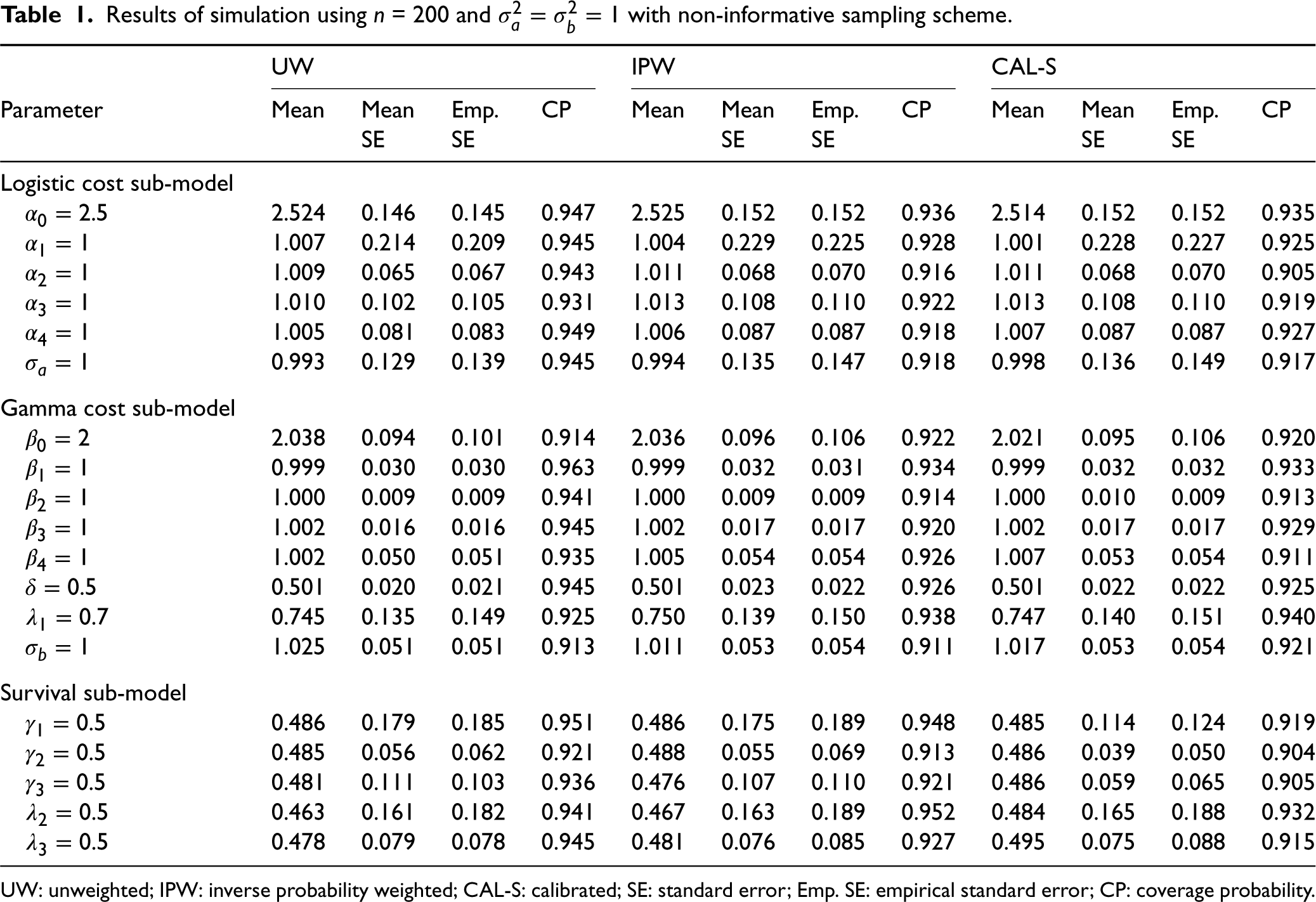
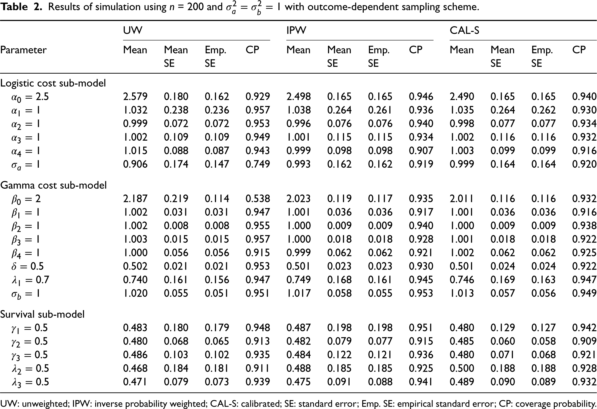
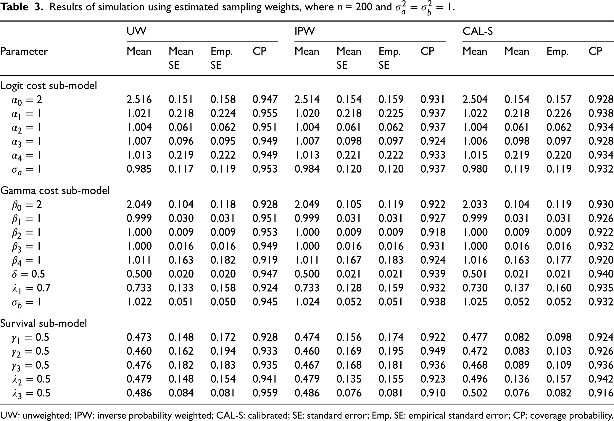
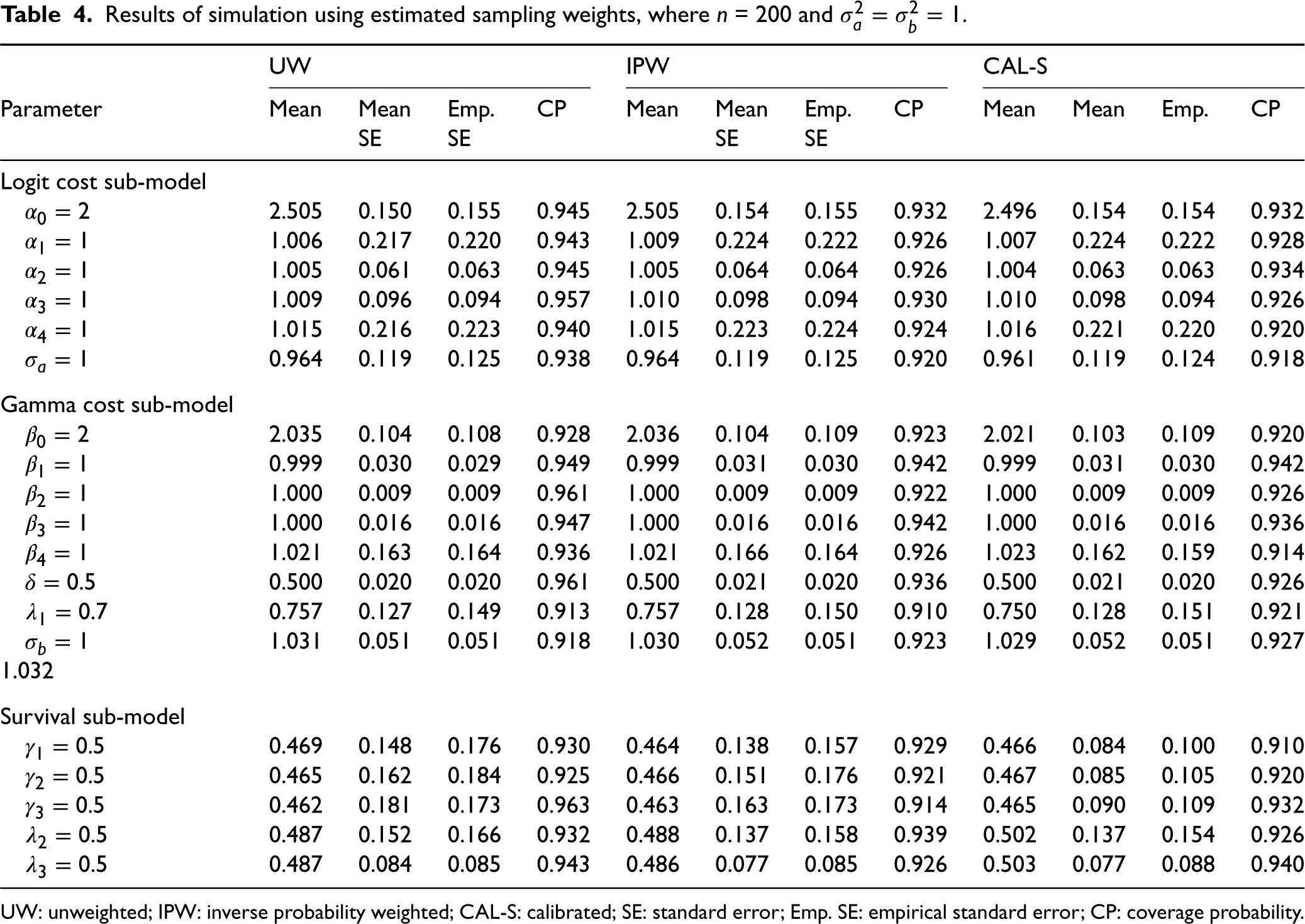
In the simulation study, the unweighted (UW), weighted (IPW) and calibrated (CAL-S) models are fit to the simulated data. The standard errors (SEs) are calculated as the square root of corresponding variance estimators as described in Section 5. Results are averaged and summarized across the 500 replicates. Results are shown in Tables 1 and 2 and provide information about the estimators in terms of SE, empirical standard error (Emp. SE) and coverage probability (CP). Tables 1 and 2 present the results from UW, IPW and CAL-S analyses using non-informative and outcome-dependent sampling schemes, respectively. IPW and CAL-S analyses in these tables are based on true sampling weights. Tables 3 and 4 present the results from UW, IPW and CAL-S analyses using different sampling schemes, respectively, using estimated weights for IPW and CAL-S analyses.

Table 1.
Results of simulation using $n$ = 200 and $σ_{a}^{2} = σ_{b}^{2} = 1$ with non-informative sampling scheme.

UW IPW CAL-S

Parameter Mean Mean Emp. CP Mean Mean Emp. CP Mean Mean Emp. CP

SE SE SE SE SE SE

Logistic cost sub-model

$α_{0} = 2.5$ 2.524 0.146 0.145 0.947 2.525 0.152 0.152 0.936 2.514 0.152 0.152 0.935

$α_{1} = 1$ 1.007 0.214 0.209 0.945 1.004 0.229 0.225 0.928 1.001 0.228 0.227 0.925

$α_{2} = 1$ 1.009 0.065 0.067 0.943 1.011 0.068 0.070 0.916 1.011 0.068 0.070 0.905

$α_{3} = 1$ 1.010 0.102 0.105 0.931 1.013 0.108 0.110 0.922 1.013 0.108 0.110 0.919

$α_{4} = 1$ 1.005 0.081 0.083 0.949 1.006 0.087 0.087 0.918 1.007 0.087 0.087 0.927

$σ_{a} = 1$ 0.993 0.129 0.139 0.945 0.994 0.135 0.147 0.918 0.998 0.136 0.149 0.917

Gamma cost sub-model

$β_{0} = 2$ 2.038 0.094 0.101 0.914 2.036 0.096 0.106 0.922 2.021 0.095 0.106 0.920

$β_{1} = 1$ 0.999 0.030 0.030 0.963 0.999 0.032 0.031 0.934 0.999 0.032 0.032 0.933

$β_{2} = 1$ 1.000 0.009 0.009 0.941 1.000 0.009 0.009 0.914 1.000 0.010 0.009 0.913

$β_{3} = 1$ 1.002 0.016 0.016 0.945 1.002 0.017 0.017 0.920 1.002 0.017 0.017 0.929

$β_{4} = 1$ 1.002 0.050 0.051 0.935 1.005 0.054 0.054 0.926 1.007 0.053 0.054 0.911

$δ = 0.5$ 0.501 0.020 0.021 0.945 0.501 0.023 0.022 0.926 0.501 0.022 0.022 0.925

$λ_{1} = 0.7$ 0.745 0.135 0.149 0.925 0.750 0.139 0.150 0.938 0.747 0.140 0.151 0.940

$σ_{b} = 1$ 1.025 0.051 0.051 0.913 1.011 0.053 0.054 0.911 1.017 0.053 0.054 0.921

Survival sub-model

$γ_{1} = 0.5$ 0.486 0.179 0.185 0.951 0.486 0.175 0.189 0.948 0.485 0.114 0.124 0.919

$γ_{2} = 0.5$ 0.485 0.056 0.062 0.921 0.488 0.055 0.069 0.913 0.486 0.039 0.050 0.904

$γ_{3} = 0.5$ 0.481 0.111 0.103 0.936 0.476 0.107 0.110 0.921 0.486 0.059 0.065 0.905

$λ_{2} = 0.5$ 0.463 0.161 0.182 0.941 0.467 0.163 0.189 0.952 0.484 0.165 0.188 0.932

$λ_{3} = 0.5$ 0.478 0.079 0.078 0.945 0.481 0.076 0.085 0.927 0.495 0.075 0.088 0.915

UW: unweighted; IPW: inverse probability weighted; CAL-S: calibrated; SE: standard error; Emp. SE: empirical standard error; CP: coverage probability.

	UW	IPW	CAL-S
Logistic cost sub-model
$α_{0} = 2.5$	2.524	0.146	0.145	0.947	2.525	0.152	0.152	0.936	2.514	0.152	0.152	0.935
$α_{1} = 1$	1.007	0.214	0.209	0.945	1.004	0.229	0.225	0.928	1.001	0.228	0.227	0.925
$α_{2} = 1$	1.009	0.065	0.067	0.943	1.011	0.068	0.070	0.916	1.011	0.068	0.070	0.905
$α_{3} = 1$	1.010	0.102	0.105	0.931	1.013	0.108	0.110	0.922	1.013	0.108	0.110	0.919
$α_{4} = 1$	1.005	0.081	0.083	0.949	1.006	0.087	0.087	0.918	1.007	0.087	0.087	0.927
$σ_{a} = 1$	0.993	0.129	0.139	0.945	0.994	0.135	0.147	0.918	0.998	0.136	0.149	0.917
Gamma cost sub-model
$β_{0} = 2$	2.038	0.094	0.101	0.914	2.036	0.096	0.106	0.922	2.021	0.095	0.106	0.920
$β_{1} = 1$	0.999	0.030	0.030	0.963	0.999	0.032	0.031	0.934	0.999	0.032	0.032	0.933
$β_{2} = 1$	1.000	0.009	0.009	0.941	1.000	0.009	0.009	0.914	1.000	0.010	0.009	0.913
$β_{3} = 1$	1.002	0.016	0.016	0.945	1.002	0.017	0.017	0.920	1.002	0.017	0.017	0.929
$β_{4} = 1$	1.002	0.050	0.051	0.935	1.005	0.054	0.054	0.926	1.007	0.053	0.054	0.911
$δ = 0.5$	0.501	0.020	0.021	0.945	0.501	0.023	0.022	0.926	0.501	0.022	0.022	0.925
$λ_{1} = 0.7$	0.745	0.135	0.149	0.925	0.750	0.139	0.150	0.938	0.747	0.140	0.151	0.940
$σ_{b} = 1$	1.025	0.051	0.051	0.913	1.011	0.053	0.054	0.911	1.017	0.053	0.054	0.921
Survival sub-model
$γ_{1} = 0.5$	0.486	0.179	0.185	0.951	0.486	0.175	0.189	0.948	0.485	0.114	0.124	0.919
$γ_{2} = 0.5$	0.485	0.056	0.062	0.921	0.488	0.055	0.069	0.913	0.486	0.039	0.050	0.904
$γ_{3} = 0.5$	0.481	0.111	0.103	0.936	0.476	0.107	0.110	0.921	0.486	0.059	0.065	0.905
$λ_{2} = 0.5$	0.463	0.161	0.182	0.941	0.467	0.163	0.189	0.952	0.484	0.165	0.188	0.932
$λ_{3} = 0.5$	0.478	0.079	0.078	0.945	0.481	0.076	0.085	0.927	0.495	0.075	0.088	0.915

Table 2.

Results of simulation using $n$ = 200 and $σ_{a}^{2} = σ_{b}^{2} = 1$ with outcome-dependent sampling scheme.

	UW				IPW				CAL-S
Parameter	Mean	Mean	Emp.	CP	Mean	Mean	Emp.	CP	Mean	Mean	Emp.	CP
		SE	SE			SE	SE			SE	SE
Logistic cost sub-model
$α_{0} = 2.5$	2.579	0.180	0.162	0.929	2.498	0.165	0.165	0.946	2.490	0.165	0.165	0.940
$α_{1} = 1$	1.032	0.238	0.236	0.957	1.038	0.264	0.261	0.936	1.035	0.264	0.262	0.930
$α_{2} = 1$	0.999	0.072	0.072	0.953	0.996	0.076	0.076	0.940	0.998	0.077	0.077	0.934
$α_{3} = 1$	1.002	0.109	0.109	0.949	1.001	0.115	0.115	0.934	1.002	0.116	0.116	0.932
$α_{4} = 1$	1.015	0.088	0.087	0.943	0.999	0.098	0.098	0.907	1.003	0.099	0.099	0.916
$σ_{a} = 1$	0.906	0.174	0.147	0.749	0.993	0.162	0.162	0.919	0.999	0.164	0.164	0.920
Gamma cost sub-model
$β_{0} = 2$	2.187	0.219	0.114	0.538	2.023	0.119	0.117	0.935	2.011	0.116	0.116	0.932
$β_{1} = 1$	1.002	0.031	0.031	0.947	1.001	0.036	0.036	0.917	1.001	0.036	0.036	0.916
$β_{2} = 1$	1.002	0.008	0.008	0.955	1.000	0.009	0.009	0.940	1.000	0.009	0.009	0.938
$β_{3} = 1$	1.003	0.015	0.015	0.957	1.000	0.018	0.018	0.928	1.001	0.018	0.018	0.922
$β_{4} = 1$	1.000	0.056	0.056	0.915	0.999	0.062	0.062	0.921	1.002	0.062	0.062	0.925
$δ = 0.5$	0.502	0.021	0.021	0.953	0.501	0.023	0.023	0.930	0.501	0.024	0.024	0.922
$λ_{1} = 0.7$	0.740	0.161	0.156	0.947	0.749	0.168	0.161	0.945	0.746	0.169	0.163	0.947
$σ_{b} = 1$	1.020	0.055	0.051	0.951	1.017	0.058	0.055	0.953	1.013	0.057	0.056	0.949
Survival sub-model
$γ_{1} = 0.5$	0.483	0.180	0.179	0.948	0.487	0.198	0.198	0.951	0.480	0.129	0.127	0.942
$γ_{2} = 0.5$	0.480	0.068	0.065	0.913	0.482	0.079	0.077	0.915	0.485	0.060	0.058	0.909
$γ_{3} = 0.5$	0.486	0.103	0.102	0.935	0.484	0.122	0.121	0.936	0.480	0.071	0.068	0.921
$λ_{2} = 0.5$	0.468	0.184	0.181	0.911	0.488	0.185	0.185	0.925	0.500	0.188	0.188	0.928
$λ_{3} = 0.5$	0.471	0.079	0.073	0.939	0.475	0.091	0.088	0.941	0.489	0.090	0.089	0.932

UW: unweighted; IPW: inverse probability weighted; CAL-S: calibrated; SE: standard error; Emp. SE: empirical standard error; CP: coverage probability.

Table 3.

Results of simulation using estimated sampling weights, where $n$ = 200 and $σ_{a}^{2} = σ_{b}^{2} = 1$ .

	UW				IPW				CAL-S
Parameter	Mean	Mean	Emp.	CP	Mean	Mean	Emp.	CP	Mean	Mean	Emp.	CP
		SE	SE			SE	SE
Logit cost sub-model
$α_{0} = 2$	2.516	0.151	0.158	0.947	2.514	0.154	0.159	0.931	2.504	0.154	0.157	0.928
$α_{1} = 1$	1.021	0.218	0.224	0.955	1.020	0.218	0.225	0.937	1.022	0.218	0.226	0.938
$α_{2} = 1$	1.004	0.061	0.062	0.951	1.004	0.061	0.062	0.937	1.004	0.061	0.062	0.934
$α_{3} = 1$	1.007	0.096	0.095	0.949	1.007	0.098	0.097	0.924	1.006	0.098	0.097	0.928
$α_{4} = 1$	1.013	0.219	0.222	0.949	1.013	0.221	0.222	0.933	1.015	0.219	0.220	0.934
$σ_{a} = 1$	0.985	0.117	0.119	0.953	0.984	0.120	0.120	0.937	0.980	0.119	0.119	0.932
Gamma cost sub-model
$β_{0} = 2$	2.049	0.104	0.118	0.928	2.049	0.105	0.119	0.922	2.033	0.104	0.119	0.930
$β_{1} = 1$	0.999	0.030	0.031	0.951	0.999	0.031	0.031	0.927	0.999	0.031	0.031	0.926
$β_{2} = 1$	1.000	0.009	0.009	0.953	1.000	0.009	0.009	0.918	1.000	0.009	0.009	0.922
$β_{3} = 1$	1.000	0.016	0.016	0.949	1.000	0.016	0.016	0.931	1.000	0.016	0.016	0.932
$β_{4} = 1$	1.011	0.163	0.182	0.919	1.011	0.167	0.183	0.924	1.016	0.163	0.177	0.920
$δ = 0.5$	0.500	0.020	0.020	0.947	0.500	0.021	0.021	0.939	0.501	0.021	0.021	0.940
$λ_{1} = 0.7$	0.733	0.133	0.158	0.924	0.733	0.128	0.159	0.932	0.730	0.137	0.160	0.935
$σ_{b} = 1$	1.022	0.051	0.050	0.945	1.024	0.052	0.051	0.938	1.025	0.052	0.052	0.932
Survival sub-model
$γ_{1} = 0.5$	0.473	0.148	0.172	0.928	0.474	0.156	0.174	0.922	0.477	0.082	0.098	0.924
$γ_{2} = 0.5$	0.460	0.162	0.194	0.933	0.460	0.169	0.195	0.949	0.472	0.083	0.103	0.926
$γ_{3} = 0.5$	0.476	0.182	0.183	0.935	0.467	0.168	0.181	0.936	0.468	0.089	0.109	0.936
$λ_{2} = 0.5$	0.479	0.148	0.154	0.941	0.479	0.135	0.155	0.923	0.496	0.136	0.157	0.942
$λ_{3} = 0.5$	0.486	0.084	0.081	0.959	0.486	0.076	0.081	0.910	0.502	0.076	0.082	0.916

UW: unweighted; IPW: inverse probability weighted; CAL-S: calibrated; SE: standard error; Emp. SE: empirical standard error; CP: coverage probability.

Table 4.

Results of simulation using estimated sampling weights, where $n$ = 200 and $σ_{a}^{2} = σ_{b}^{2} = 1$ .

	UW				IPW				CAL-S
Parameter	Mean	Mean	Emp.	CP	Mean	Mean	Emp.	CP	Mean	Mean	Emp.	CP
		SE	SE			SE	SE
Logit cost sub-model
$α_{0} = 2$	2.505	0.150	0.155	0.945	2.505	0.154	0.155	0.932	2.496	0.154	0.154	0.932
$α_{1} = 1$	1.006	0.217	0.220	0.943	1.009	0.224	0.222	0.926	1.007	0.224	0.222	0.928
$α_{2} = 1$	1.005	0.061	0.063	0.945	1.005	0.064	0.064	0.926	1.004	0.063	0.063	0.934
$α_{3} = 1$	1.009	0.096	0.094	0.957	1.010	0.098	0.094	0.930	1.010	0.098	0.094	0.926
$α_{4} = 1$	1.015	0.216	0.223	0.940	1.015	0.223	0.224	0.924	1.016	0.221	0.220	0.920
$σ_{a} = 1$	0.964	0.119	0.125	0.938	0.964	0.119	0.125	0.920	0.961	0.119	0.124	0.918
Gamma cost sub-model
$β_{0} = 2$	2.035	0.104	0.108	0.928	2.036	0.104	0.109	0.923	2.021	0.103	0.109	0.920
$β_{1} = 1$	0.999	0.030	0.029	0.949	0.999	0.031	0.030	0.942	0.999	0.031	0.030	0.942
$β_{2} = 1$	1.000	0.009	0.009	0.961	1.000	0.009	0.009	0.922	1.000	0.009	0.009	0.926
$β_{3} = 1$	1.000	0.016	0.016	0.947	1.000	0.016	0.016	0.942	1.000	0.016	0.016	0.936
$β_{4} = 1$	1.021	0.163	0.164	0.936	1.021	0.166	0.164	0.926	1.023	0.162	0.159	0.914
$δ = 0.5$	0.500	0.020	0.020	0.961	0.500	0.021	0.020	0.936	0.500	0.021	0.020	0.926
$λ_{1} = 0.7$	0.757	0.127	0.149	0.913	0.757	0.128	0.150	0.910	0.750	0.128	0.151	0.921
$σ_{b} = 1$	1.031	0.051	0.051	0.918	1.030	0.052	0.051	0.923	1.029	0.052	0.051	0.927
1.032
Survival sub-model
$γ_{1} = 0.5$	0.469	0.148	0.176	0.930	0.464	0.138	0.157	0.929	0.466	0.084	0.100	0.910
$γ_{2} = 0.5$	0.465	0.162	0.184	0.925	0.466	0.151	0.176	0.921	0.467	0.085	0.105	0.920
$γ_{3} = 0.5$	0.462	0.181	0.173	0.963	0.463	0.163	0.173	0.914	0.465	0.090	0.109	0.932
$λ_{2} = 0.5$	0.487	0.152	0.166	0.932	0.488	0.137	0.158	0.939	0.502	0.137	0.154	0.926
$λ_{3} = 0.5$	0.487	0.084	0.085	0.943	0.486	0.077	0.085	0.926	0.503	0.077	0.088	0.940

UW: unweighted; IPW: inverse probability weighted; CAL-S: calibrated; SE: standard error; Emp. SE: empirical standard error; CP: coverage probability.

Our simulation results in Table 1 show that when the sampling design is non-informative, using the unweighted log-likelihood (the standard maximum likelihood estimation) leads to a small finite sample bias. Using the log-pseudolikelihood also leads to unbiased results, with a slightly greater amount of variability of estimators. This indicates efficiency loss from multiplying the sampling weights by the individual likelihood contribution when there is no need to consider the sampling design, and is consistent with the result by Xu et al. As expected, Table 1 in the Supplemental Material shows that increasing the phase-two sample size $n$ from 200 to 400 leads to significant efficiency gains in all estimators.

Our simulation results in Table 2 indicate that under the outcome-dependent sampling scheme, using the unweighted log-likelihood leads to biased estimates for model intercepts $α_{0}$ and $β_{0}$ . This is because under the outcome-dependent sampling scheme, given the covariate $Z$ , subjects with larger amount of costs are oversampled, which leads to overestimated intercepts ${\hat{α}}_{0}$ and ${\hat{β}}_{0}$ in the cost sub-models, when the sampling design is not considered. Using the joint log-pseudolikelihood eliminates the bias present in the estimates of the model intercepts from using the unweighted model that ignores that sampling design, with a slight loss in efficiency. As the unweighted model leads to biased estimates for the model intercepts, we report MSE (mean squared error) in place of model-based SE. This shows that, in order to obtain a small finite sample bias, sampling designs should be reflected in the statistical analysis when making inferences about a sample obtained using an outcome-dependent sampling scheme.

Under both non-informative and outcome-dependent sampling scheme, calibration to surrogates of the survival model influence functions leads to significant efficiency gains for the parameter estimates ( ${\hat{γ}}_{1}, {\hat{γ}}_{2}, {\hat{γ}}_{3})^{T}$ associated with the survival model. As expected, calibration to surrogates of the survival model influence functions does not seem to lead to significant efficiency gains or loss for the parameter estimates of interest ( ${\hat{α}}_{0}, {\hat{α}}_{1}, {\hat{α}}_{2}, {\hat{α}}_{3}, {\hat{α}}_{4})^{T}$ and ( ${\hat{β}}_{0}, {\hat{β}}_{1}, {\hat{β}}_{2}, {\hat{β}}_{3}, {\hat{β}}_{4})^{T}$ in the cost models, including ${\hat{α}}_{4}$ and ${\hat{β}}_{4}$ , which are parameter estimates associated with the individual-level variable common to all sub-models, despite the interdependence of the sub-models via shared random effects.

Tables 3 and 4 show our simulation results where IPW and CAL-S analyses are based on estimated weights. The simulation studies in both tables are based on the identical weight estimation model, using sampling schemes (21) and (22), respectively. Tables 3 and 4 indicate that under both scenarios using estimated weights, as expected, pseudolikelihood estimator does not lead to significant efficiency gains or loss compared to the unweighted estimator. However, both unweighted and unweighted models lead to a small finite sample bias, even when the weight estimation model is incorrectly specified and does not correctly reflect the variables used in the phase-two sample selection.

Calibration to surrogates of the survival model influence functions under estimated weights leads to significant efficiency gains in the parameters estimates ( ${\hat{γ}}_{1}, {\hat{γ}}_{2}, {\hat{γ}}_{3})^{T}$ associated with the survival model, which is consistent with our simulation results that use true sampling weights.

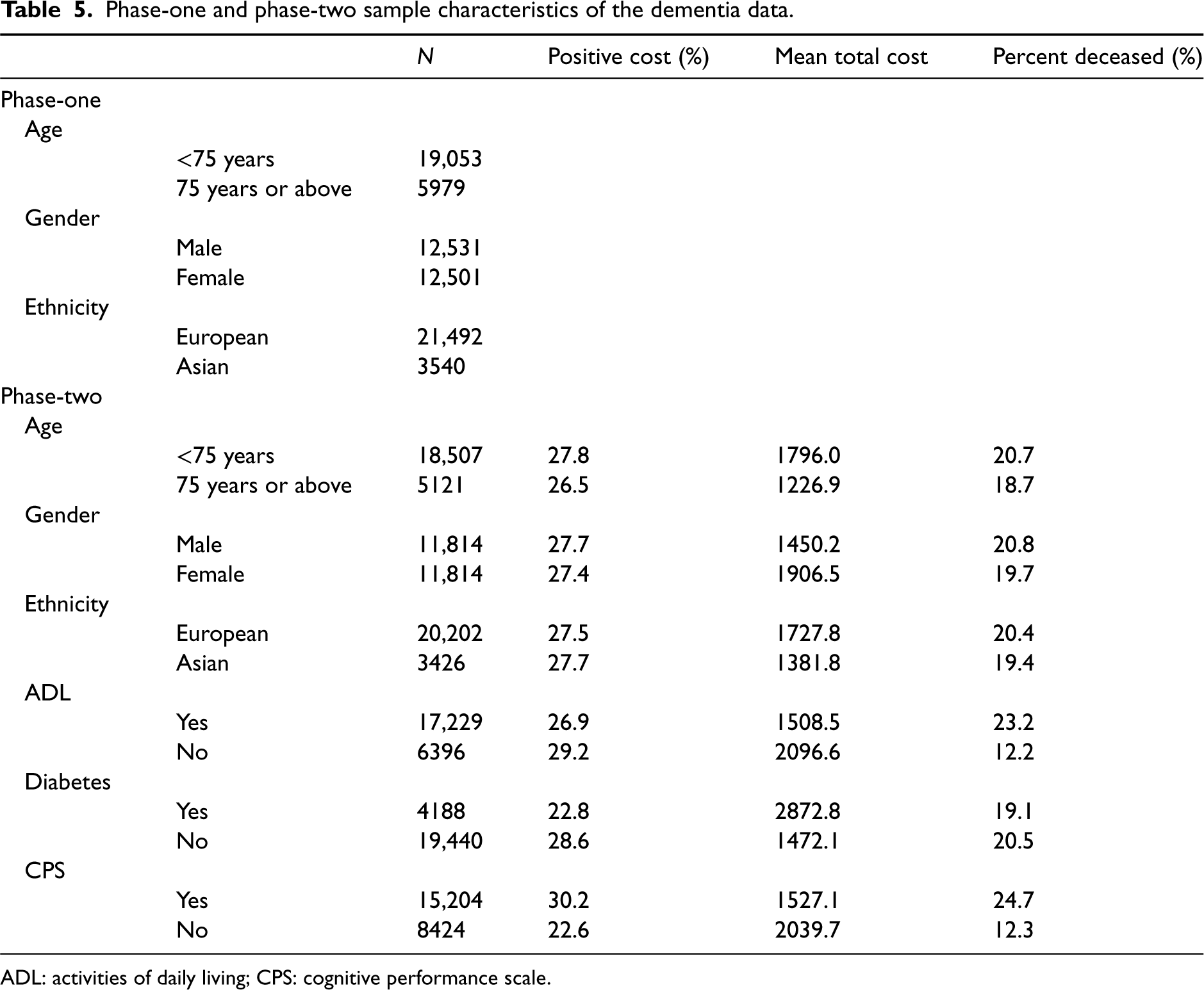
We conclude that calibration to surrogates of the influence functions from the survival model leads to significant efficiency gains for ( ${\hat{γ}}_{1}, {\hat{γ}}_{2}, {\hat{γ}}_{3})^{T}$ compared to the unweighted and weighted analysis. We also conclude that calibrating the survival model in a joint model setting does not lead to any significant efficiency gains for the parameters in the cost models including the parameters for the shared individual-level variable, compared to the unweighted and weighted analysis.

7. Application to anti-dementia medication cost and mortality data for people with diagnosed dementia in New Zealand

We apply our proposed method to jointly model anti-dementia medication costs and mortality in people with diagnosed dementia in New Zealand. We use an integrated dataset which was integrated from multiple datasets managed by Stats NZ Integrated Data Infrastructure (IDI) and interRAI.

Table 5 shows the phase-one and phase-two sample characteristics of the dementia data. For the phase-one sample, demographic information that includes age, gender and ethnicity is available, and for the phase-two sample, additional information that includes positive medication cost and mortality outcome is available. All phase-one sample individuals that are not included in the phase-two sample were not prescribed medications and are alive. In this application, mortality, its risk factors and determinants of anti-dementia medication costs are investigated for people with diagnosed dementia in New Zealand. The covariates of interest are age, gender, ethnicity, diabetes diagnosis, ADL (Activities of Daily Living) dependence and CPS (Cognitive Performance Scale). Many elderly, including those with diagnosed dementia, are disabled in one of more activities of daily living (ADL) such as bathing, eating and dressing. It is also of interest to evaluate the estimation of association parameters $(λ_{1}, λ_{2}, λ_{3})^{T}$ to investigate whether the probability of incurring anti-dementia medication cost, the amount incurred and mortality are associated.

Table 5.
Phase-one and phase-two sample characteristics of the dementia data.

$N$ Positive cost (%) Mean total cost Percent deceased (%)

Phase-one

Age

<75 years 19,053

75 years or above 5979

Gender

Male 12,531

Female 12,501

Ethnicity

European 21,492

Asian 3540

Phase-two

Age

<75 years 18,507 27.8 1796.0 20.7

75 years or above 5121 26.5 1226.9 18.7

Gender

Male 11,814 27.7 1450.2 20.8

Female 11,814 27.4 1906.5 19.7

Ethnicity

European 20,202 27.5 1727.8 20.4

Asian 3426 27.7 1381.8 19.4

ADL

Yes 17,229 26.9 1508.5 23.2

No 6396 29.2 2096.6 12.2

Diabetes

Yes 4188 22.8 2872.8 19.1

No 19,440 28.6 1472.1 20.5

CPS

Yes 15,204 30.2 1527.1 24.7

No 8424 22.6 2039.7 12.3

ADL: activities of daily living; CPS: cognitive performance scale.

		$N$	Positive cost (%)	Mean total cost	Percent deceased (%)
Phase-one
Age
	<75 years	19,053
	75 years or above	5979
Gender
	Male	12,531
	Female	12,501
Ethnicity
	European	21,492
	Asian	3540
Phase-two
Age
	<75 years	18,507	27.8	1796.0	20.7
	75 years or above	5121	26.5	1226.9	18.7
Gender
	Male	11,814	27.7	1450.2	20.8
	Female	11,814	27.4	1906.5	19.7
Ethnicity
	European	20,202	27.5	1727.8	20.4
	Asian	3426	27.7	1381.8	19.4
ADL
	Yes	17,229	26.9	1508.5	23.2
	No	6396	29.2	2096.6	12.2
Diabetes
	Yes	4188	22.8	2872.8	19.1
	No	19,440	28.6	1472.1	20.5
CPS
	Yes	15,204	30.2	1527.1	24.7
	No	8424	22.6	2039.7	12.3

In this application, true sampling weights are not available as there is no intervention in the phase-two sample selection and estimated weights and their calibrated weights are used to derive IPW and calibrated estimators, respectively. For calibration, we use ADL dependence, CPS and diabetes diagnosis as target variables, as they are only known in the phase-two sample, and demographics including age, gender and ethnicity as auxiliary variables, which are known in the phase-one sample.

The results in Table 6 show that dementia patients with higher CPS are more likely to use anti-dementia medication $(p =< 0.001)$ , incur higher anti-dementia medication cost $(p =< 0.001)$ , and die $(p =< 0.001)$ . Patients with ADL dependence were less likely to use anti-dementia medications and more likely to incur less cost for such medications, but were more likely to die $(p =< 0.001)$ .

Table 6.

Parameter estimates and SEs for dementia data using calibrated log-pseudolikelihood.

	UW			IPW			CAL-S
Variable	Estimate	SE	p-value	Estimate	SE	p-value	Estimate	SE	p-value
Probability of non-zero cost
Intercept	−7.377	0.110	<0.001	−7.423	0.108	<0.001	−7.424	0.110	<0.001
ADL	−0.376	0.097	<0.001	−0.375	0.096	<0.001	−0.376	0.097	<0.001
Diabetes	−0.315	0.110	0.004	−0.315	0.110	0.004	−0.315	0.110	0.004
CPS	0.569	0.092	<0.001	0.567	0.093	<0.001	0.569	0.093	<0.001
Age: 75+	−0.087	0.100	0.383	−0.200	0.100	0.047	−0.198	0.100	0.048
Female	−0.007	0.081	0.932	−0.002	0.081	0.976	−0.002	0.081	0.975
Asian	−0.011	0.116	0.923	−0.008	0.116	0.948	−0.008	0.116	0.948
Amount of cost
Intercept	0.598	0.038	<0.001	0.581	0.039	<0.001	0.581	0.039	<0.001
ADL	−0.115	0.011	<0.001	−0.114	0.011	<0.001	−0.114	0.011	<0.001
Diabetes	0.031	0.013	0.017	0.030	0.013	0.021	0.030	0.013	0.020
CPS	0.083	0.011	<0.001	0.083	0.011	<0.001	0.083	0.011	<0.001
Age:75+	−0.045	0.011	<0.001	−0.074	0.012	<0.001	−0.074	0.012	<0.001
Female	−0.029	0.009	0.001	−0.028	0.009	0.0025	−0.028	0.009	0.002
Asian	−0.010	0.013	0.438	−0.009	0.013	0.494	−0.009	0.013	0.492
Survival
ADL	0.537	0.041	<0.001	0.563	0.040	<0.001	0.537	0.041	<0.001
Diabetes	−0.012	0.039	0.752	−0.013	0.038	0.733	−0.013	0.039	0.736
CPS	0.567	0.037	<0.001	0.568	0.036	<0.001	0.567	0.037	<0.001
Age:75+	−0.077	0.037	0.036	−0.076	0.034	0.027	−0.144	0.007	<0.001
Female	−0.060	0.029	0.040	−0.061	0.028	0.031	−0.061	0.006	<0.001
Asian	−0.083	0.042	0.049	−0.083	0.042	0.046	−0.079	0.008	<0.001
Variance component
$σ_{a}$	9.470	0.110	<0.001	9.535	0.110	<0.001	9.536	0.110	<0.001
$σ_{b}$	0.335	0.090	<0.001	0.343	0.090	<0.001	0.342	0.090	<0.001
Association parameters
$λ_{1}$	0.232	0.003	<0.001	0.232	0.003	<0.001	0.232	0.004	<0.001
$λ_{2}$	−0.014	0.003	<0.001	−0.014	0.003	<0.001	−0.014	0.003	$< 0.001$
$λ_{3}$	−0.041	0.043	0.350	0.016	0.046	0.727	0.016	0.047	0.727

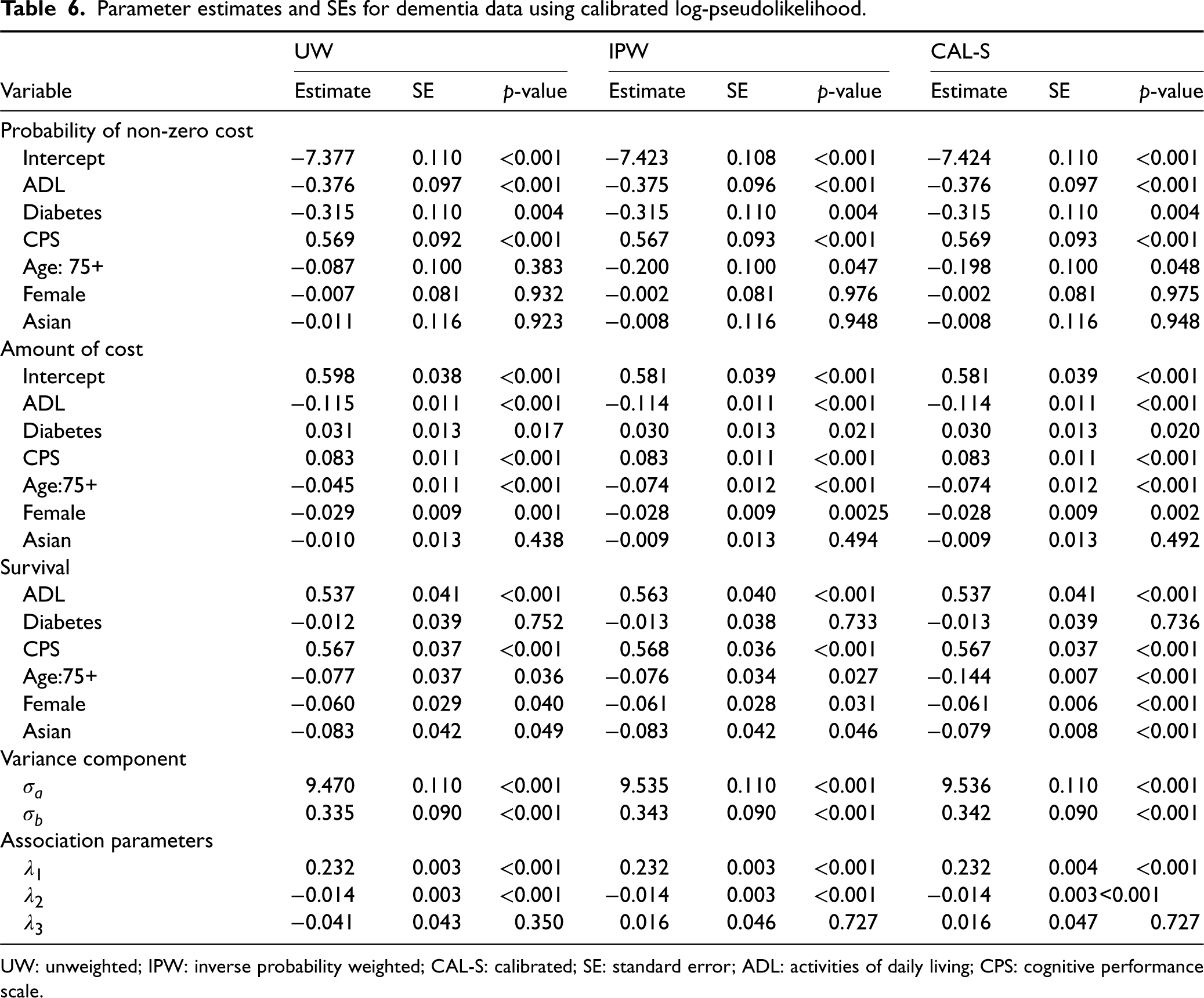
UW: unweighted; IPW: inverse probability weighted; CAL-S: calibrated; SE: standard error; ADL: activities of daily living; CPS: cognitive performance scale.

Patients who were 75 years old or younger were more likely to die compared to those older than 75 years old, which is consistent with previous findings that early onset dementia leads to higher mortality.³⁰ In addition, Asian ethnicity and being female were associated with lower mortality in dementia patients. There was no statistically significant differences in anti-dementia medication use between males and females which supports previous findings.³¹

The estimated coefficient of the parameter $λ_{1}$ that associates the random effect $a$ to the amount of medication cost were small in magnitude for both IPW and CAL-S analyses, but was highly significant ( $p =< 0.001)$ . This suggests that there is association between probability of incurring anti-dementia pharmaceutical costs and the amount of anti-dementia pharmaceutical costs.

In all analyses, ${\hat{σ}}_{b}$ , the estimated variance of the random effect $b$ , had a small magnitude but was highly significant ( $p =< 0.001)$ , suggesting that there is additional heterogeneity in anti-dementia medication cost not completely explained by the random effect $a$ . In addition, $λ_{3}$ , which is the parameter that associates the random effect $b$ to survival was not significant in all types of analyses. This indicates that there exists additional heterogeneity in the amount of anti-dementia medication cost that is not related to mortality.

As expected, calibration to surrogates of the survival model influence functions led to significant efficiency gains in the estimates of phase-one variables (age, gender and ethnicity) on mortality in the survival model. There were no efficiency gains in the estimates of phase-two variables, as the phase-one variables did not have a high correlation with the phase-two variables. This calibration methodology did not lead to any efficiency gains or loss in the parameters associated with the cost models. These results are expected based on our simulation studies where calibration to surrogates of the survival model influence functions only led to efficiency gains in the estimates of survival model parameters $({\hat{γ}}_{1}, {\hat{γ}}_{2}, {\hat{γ}}_{3})^{T}$ , but did not lead to gains nor loss in the parameters associated with the cost sub-models.

8. Discussion

Medical cost data are usually obtained using complex sampling designs rather than SRS and are characterized by right skewness and excessive proportion of zeros. These characteristics need to be reflected in the statistical analysis of medical cost data for valid statistical inference. In addition, medical cost is associated with survival as patients with a greater amount of medical cost are less likely to survive, and it is important that a joint model is used to analyse the two data types simultaneously to obtain more efficient parameter estimates compared to separate analysis of the two data types.

In this article, we extended the pseudolikelihood approach by Xu et al. to jointly model medical cost and mortality for complex surveys using survey calibration that modifies the sampling weights in a joint model setting. For calibration, we used surrogates by the influence functions from the survival sub-model fitted using imputed phase-one target variable and phase-one auxiliary variables. Such surrogates of the survival model influence functions were used to calibrate the sampling weights for the phase-two sample and estimate variances of the parameter estimates.

We showed that calibration to surrogates of the survival model influence functions led to efficiency gains for the parameters in the survival sub-model but not for the parameters in the cost sub-models, including the shared individual-level variable, despite the fact the sub-models are associated via shared random effects. This type of calibration is useful when the main interest is in making inferences about the survival model in a joint model setting, as we can gain significant efficiency gains for the survival model parameter estimates while accounting for the association between time-to-event and the longitudinal outcome variable. In order to make inferences about the survival model in a joint model setting, we recommend using calibration to surrogates of the survival model influence functions, for further efficiency gains.

A potential future work may be based on weight calibration in a joint model setting where the level of correlation between the longitudinal variable and survival is high, which leads to greater dependency between the sub-models. For potential application to real data where longitudinal and survival outcomes that are highly correlated are available, it may be of interest to investigate whether only using surrogates of the influence functions from the survival model can lead to efficiency gains in the longitudinal models.

Supplemental Material

sj-pdf-1-smm-10.1177_09622802241236935 - Supplemental material for Weight calibration in the joint modelling of medical cost and mortality

Supplemental material, sj-pdf-1-smm-10.1177_09622802241236935 for Weight calibration in the joint modelling of medical cost and mortality by Seong Hoon Yoon, Alain Vandal and Claudia Rivera-Rodriguez in Statistical Methods in Medical Research

Footnotes

Acknowledgements

This work was supported in part by the University of Auckland doctoral scholarship (to the first author). The authors wish to acknowledge the use of New Zealand eScience Infrastructure (NeSI) high performance computing facilities, consulting support and/or training services as part of this research. New Zealand’s national facilities are provided by NeSI and funded jointly by NeSI’s collaborator institutions and through the Ministry of Business, Innovation & Employment’s Research Infrastructure programme. .

Declaration of conflicting interests

The author(s) declared no potential conflicts of interest with respect to the research, authorship, and/or publication of this article.

Funding

The author(s) received no financial support for the research, authorship, and/or publication of this article.

Data availability

Data may be obtained from a third party and is not publicly available. Access to the data used in this research can be applied through Statistics New Zealand. .

ORCID iDs

Seong Hoon Yoon

Claudia Rivera-Rodriguez

Supplemental material

Supplemental material for this article is available online.

References

Sudell

Kolamunnage-Dona

Tudur-Smith

. Joint models for longitudinal and time-to-event data: a review of reporting quality with a view to meta-analysis. BMC Med Res Methodol 2016 Dec 5; 16: 168.

Liu

Grace

, et al. Analysis of longitudinal and survival data: joint modeling, inference methods, and issues. J Probab Stat 2012; 2012: 1–17.

Slasor

Laird

. Joint models for efficient estimation in proportional hazards regression models. Stat Med 2003 Jul 15; 22: 2137–2148. DOI: 10.1002/sim.1439. PMID: 12820279.

Caruana

Roman

Hernández-Sánchez

et al. Longitudinal studies. J Thorac Dis 2015; 7: E537–E540.

Schober

Vetter

. Survival analysis and interpretation of time-to-event data: the tortoise and the hare. Anesth Analg 2018; 127: 792–798.

Ibrahim

Chu

Chen

. Basic concepts and methods for joint models of longitudinal and survival data. J Clin Oncol: Official J Am Soc Clin Oncol 2010; 28: 2796–2801.

Tsiatis

DeGruttola

Wulfsohn

. Modeling the relationship of survival to longitudinal data measured with error. Applications to survival and CD4 counts in patients with AIDS. J Am Stat Assoc 1995; 90: 27–37.

Rizopoulos

. Joint Models for Longitudinal and Time-to-Event Data, With Applications in R. Boca Raton: Chapman and Hall/CRC, 2012.

Daggy

et al. Joint modeling of medical cost and survival in complex sample surveys. Stat Med 2013; 32: 1509–1523.

10.

Breslow

Lumley

Ballantyne

et al. Improved Horvitz–Thompson estimation of model parameters from two-phase stratified samples: applications in epidemiology. Stat Biosci 2009; 1: 32–49.

11.

Neyman

. Contribution to the theory of sampling human populations. J Am Stat Assoc 1938; 33: 101–116.

12.

Breslow

Chatterjee

. Design and analysis of two-phase studies with binary outcome applied to wilms tumour prognosis. J R Stat Soc Series C (Applied Statistics) 1999; 48: 457–468.

13.

Tao

Mercaldo

Haneuse

et al. Two-wave two-phase outcome-dependent sampling designs, with applications to longitudinal binary data. Stat Med 2021; 40: 1863–1876.

14.

Breslow

Wellner

. Weighted likelihood for semiparametric models and two-phase stratified samples, with application to Cox regression. Scandinavian J Stat 2007; 34: 86–102.

15.

Liu

Strawderman

Cowen

et al. A flexible two-part random effects model for correlated medical costs. J Health Econ 2010; 29: 110–123.

16.

. Mixed Effects Models for Complex Data. Boca Raton: Chapman & Hall/CRC, 2009.

17.

Hahs-Vaughn

. A primer for using and understanding weights with national datasets. J Exp Educ 2005; 73: 221–248.

18.

Kneipp

Yarandi

. Complex sampling designs and statistical issues in secondary analysis. West J Nurs Res 2002; 24: 552–566.

19.

Thomas

Heck

. Analysis of large-scale secondary data in higher education research: potential perils associated with complex sampling designs. Res High Educ 2001; 42: 517–540.

20.

Murphy

van der Vaart

. On profile likelihood. J Am Stat Assoc 2000; 95: 449–465.

21.

Deville

Särndal

. Calibration estimators in survey sampling. J Am Stat Assoc 1992; 87: 376–382.

22.

Lumley

Shaw

Dai

. Connections between survey calibration estimators and semiparametric models for incomplete data. Int Stat Rev 2011; 79: 200–220.

23.

Breslow

Lumley

Ballantyne

et al. Using the whole cohort in the analysis of casecohort data. Am J Epidemiol 2009; 169: 1398–1405.

24.

Rivera

Lumley

. Using the whole cohort in the analysis of countermatched samples. Biometrics 2016; 72: 382–391.

25.

Therneau

Grambsch

. Modelling Survival Data: Extending the Cox Model. New York: Springer, 2000.

26.

Kulich

Lin

. Improving the efficiency of relative-risk estimation in case-cohort studies. J Am Stat Assoc 2004; 99: 832–844.

27.

Lumley

. Complex Surveys: A Guide to Analysis Using R. Hoboken, Washington: John Wiley & Sons, 2011.

28.

Kristensen

Nielsen

Berg

et al. TMB: automatic differentiation and Laplace approximation. J Stat Softw 2016; 70: 1–21.

29.

Robins

Rotnitzky

Zhao

. Estimation of regression coefficients when some regressors are not always observed. J Amer Statist Assoc 1994; 89: 846–866.

30.

Koedam

Pijnenburg

Deeg

et al. Early-onset dementia is associated with higher mortality. Dement Geriatr Cogn Disord 2008; 26: 147–152.

31.

Chan

AHY

Hikaka

et al. anti-dementia medication use in Aotearoa New Zealand: An exploratory study using health data from the integrated data infrastructure (IDI). Aust N Z J Psychiatry 2023; 57: 895–903.

Supplementary Material

Please find the following supplemental material available below.

For Open Access articles published under a Creative Commons License, all supplemental material carries the same license as the article it is associated with.

For non-Open Access articles published, all supplemental material carries a non-exclusive license, and permission requests for re-use of supplemental material or any part of supplemental material shall be sent directly to the copyright owner as specified in the copyright notice associated with the article.

0.00 MB

0.12 MB