
Abstract
The identification of biomarkers for disease onset in longitudinal studies necessitates precise estimation of the association between longitudinal markers and survival outcomes. Currently, methods for estimating these associations in the context of left-truncated and clustered survival outcomes are lacking. In this study, we propose a novel model tailored to this scenario and develop several estimation methods: last observation carried forward, regression calibration, and a two-stage likelihood approach for joint modeling of longitudinal and survival processes. Simulation results indicate that the last observation carried forward method performs well only with a dense grid and no marker measurement error. For less dense grids and low measurement error, regression calibration approaches are preferred. Joint modeling approaches outperform calibration methods in the presence of measurement error, although they may suffer from numerical instability. In cases of numerical instability, calibration methods might be a good alternative. We applied these methodologies to the TwinsUK data to estimate the effect of bone mineral density (BMD) as a longitudinal marker on fracture incidence in 766 elderly females, 138 of whom experienced a fracture. The survival model included a shared gamma-distributed frailty to account for correlation between the times to fracture of twin pairs. Estimates obtained using calibration and joint modeling approaches indicated a larger BMD effect compared to the last observation carried forward method, likely due to the irregular BMD measurement process and minimal measurement error. Overall, our methods offer valuable tools for modeling the effect of a longitudinal marker on survival outcomes in complex designs.
Introduction
Modeling the relationship between a longitudinal marker and a time-to-event outcome is a popular research area. To date, most of this research has focused on modeling data from independent subjects (singletons), using time-in-study (follow-up time) as the primary time scale. For many diseases, however, age is the natural time scale, which results in left truncation of the time-to-event outcome. Additionally, longitudinal data collection often follows complex designs. Twin studies, as one of the most prominent sources of high-quality longitudinal data,1,2 present unique challenges due to their clustered nature. This paper focuses on estimating the association between a longitudinal marker and a left-truncated survival outcome in twin studies. Currently, no method exists to handle this type of data.
A common approach to model dependence of clustered event times is by introducing a cluster-specific random effect—the shared frailty model.3–6 The survival times are assumed to be conditionally independent given the shared (common) frailty. The gamma distribution has commonly been considered for the frailties because of mathematical convenience, since it typically produces a tractable marginal likelihood function for the parameters after integration. The literature on joint models for a longitudinal marker and a survival outcome in paired data is limited, and currently used models lack flexibility. Specifically, in the models of Ratcliffe et al.,
7
and Brilleman et al.,
8
the correlation between the survival times of cluster members is solely modeled by the normally distributed shared effects of the survival and longitudinal outcomes. This model can be fitted using the available statistical software (e.g.,
Estimation of the parameters of joint models by maximum likelihood is time-consuming due to the necessary numerical integration of the normally distributed shared random effects in the survival model. 14 Using a novel two-stage joint likelihood approach, we propose to jointly estimate the shared random effect of the longitudinal marker and the frailty term of the survival process, preceded by the plug-in of the best linear unbiased predictions (BLUP) estimates for the individual-specific random effects of the longitudinal marker.
Furthermore, for estimation of the relationship between the longitudinal marker and the survival outcome, we compare the performance of this new joint modeling (JM) approach with two classical and simpler approaches adapted to clustered and left-truncated data, namely the last observation carried forward (LOCF) approach and regression calibration techniques. In the context of independent data, and under the strong assumption that the longitudinal process only jumps at observed time points and remains constant between two consecutive observation points, the LOCF approach has been proposed for modeling the relationship between the marker and the time-to-event outcome in singletons. This method can be easily extended to clustered data by using shared frailty models, which can be fitted using available statistical packages (e.g., the
Methods have been developed for shared-frailty models, but are restricted to time-fixed covariates. Hence, there is no software available to estimate the effect of a longitudinal marker on a time-to-event outcome by the LOCF approach on clustered data with delayed entry. Here, we extend the method for time-fixed covariates to the context of longitudinal markers. Often, the assumption of constant values within observation intervals cannot be made. For such cases, regression calibration methods have been proposed for singletons.16–22 These are two-step approaches consisting of first fitting a mixed model to obtain estimates of the longitudinal marker. These estimated values can then be used in a second step as if they had been observed in the LOCF-based approach. Here, we extend regression calibration methods to the context of frailty models with delayed entry, which requires a more complex first step involving a linear mixed model with extra random effects to model the correlation between the longitudinal outcomes of cluster members. Using an intensive simulation study, we provide specific recommendations for estimation methods, taking into account the underlying model, the time gaps between longitudinal observations, and the level of measurement error.
As a data example, we consider bone mineral density (BMD), repeatedly measured over time, and the risk of fracture for twins from the TwinsUK registry. In a previous paper, we estimated the probability of a fracture in the next time period given current age and BMD using shared frailty models. 23 For such a question, follow-up time is the natural underlying time variable. Here, we are interested in modeling the effect of BMD on fracture incidence. As with many other aging-related diseases, for such a model, age is the natural time scale, which, in combination with twins entering the registry at different ages (delayed entry), results in left truncation of the time-to-event outcome.
The contributions of this paper are threefold. Firstly, it presents a novel statistical model for the analysis of longitudinal and survival data in twins. Secondly, it introduces a new set of estimation methods, each offering increased flexibility and computational complexity, all adapted to deal with left-truncated survival data. Thirdly, it provides users with guidance based on simulation results, advising on the choice of the estimation method according to factors such as observation grid density and measurement error.
The rest of this paper is laid out as follows: in the second section, we formalize the problem and propose novel approaches, in the third section, we study the performance of the methods via simulations, in the fourth section we present the results of the analysis of the TwinsUK dataset to estimate the effect of BMD on age-specific fracture incidence using our novel approaches. Lastly, the fifth section provides the discussion and conclusions.
Methods
Notation and model formulation
We are interested in modeling the relationship between a longitudinal marker and survival times in twin pairs. Let
Depending on the available amount of information on


Typically,

Now, to model the relationship between
Firstly, we consider the case that


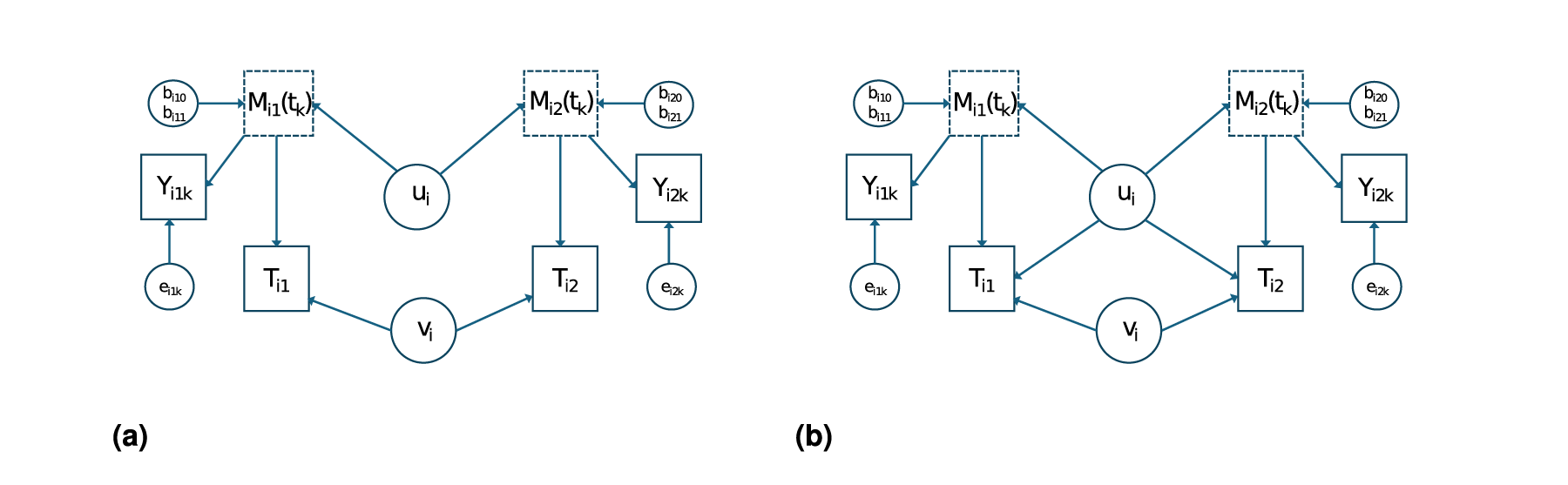
Model for the relationship between the marker profile
Let
Estimation of
by LOCF
When it can be assumed that the observations
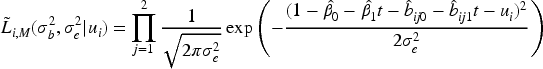
Assume that the longitudinal marker

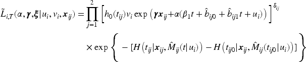
For this model, the contribution of the
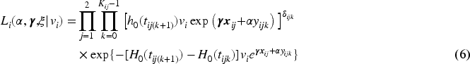
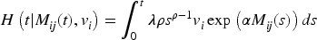
To obtain the marginal likelihood, we have to integrate over the distribution of the frailty

This approach is called LOCF since at event time
When it cannot be assumed that

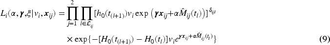
To obtain the necessary estimates for equation (8), a model can be fitted using all data under the assumption that the marker profiles are not influenced by the dropout due to the occurrence of the event. This method is called ordinary regression calibration (ORC;16–22). If this assumption cannot be made, a way to relax it is to fit a model for each time point
For


To summarize, for estimation of the effect of a longitudinal marker on a survival time in clusters subject to delayed entry, we have proposed four new methods, namely LOCF, ORC, RCC, and JM. The calibration methods ORC and RCC estimate the marker value for each individual for a grid of time points, either using one linear mixed model for all data (ORC) or by using separate models for each time point (RCC). The last two-stage method (JM) estimates only a part of the parameters of the model for
We evaluate and compare the bias of the presented estimators across various approaches, considering both sparse and dense scenarios, and the presence or absence of measurements. To do so, we simulate from a joint model for longitudinal and time-to-event data. Suppose that there are G groups with


We assume that right censoring follows a uniform distribution
The following parameter values are used
We report the relative bias (reBias) and standard deviation (SD) for estimation of parameters in 1000 Monte Carlo trials for LOCF, regression calibration, and joint model in the main text. Results for mean square error (MSE) and coverage probabilities (CPs) are given in the Appendix. All methods are fit on the same simulated datasets. Inc.G represents the number of clusters included in the analysis after truncation and after removal of singletons (i.e., we only consider fully observed clusters). For all models, we fit a Weibull proportional hazards model.
Scenario 1: Dense and no measurement error
For this scenario, the longitudinal measurements are taken with a regular gap of 2 for all individuals, that is, at regular time points
Scenario 2: Sparse and no measurement error
For this scenario, all individuals have three or fewer measurements (i.e.,
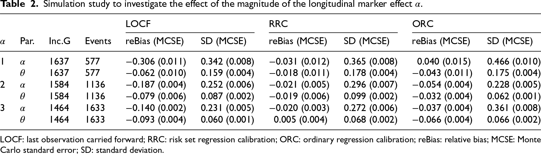
Simulation study to investigate the effect of the magnitude of the longitudinal marker effect
.
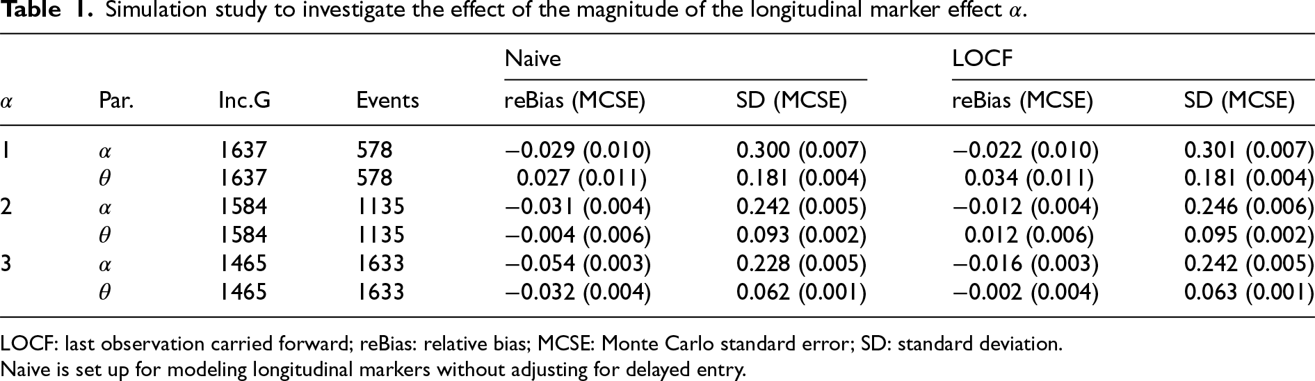
Simulation study to investigate the effect of the magnitude of the longitudinal marker effect
LOCF: last observation carried forward; reBias: relative bias; MCSE: Monte Carlo standard error; SD: standard deviation.
Naive is set up for modeling longitudinal markers without adjusting for delayed entry.
The results are depicted in Table 2 and in Table 7 in the Appendix. LOCF appeared to perform better for larger values of
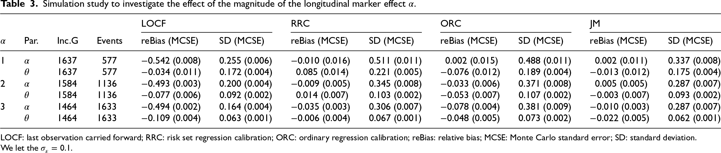
Simulation study to investigate the effect of the magnitude of the longitudinal marker effect
LOCF: last observation carried forward; RRC: risk set regression calibration; ORC: ordinary regression calibration; reBias: relative bias; MCSE: Monte Carlo standard error; SD: standard deviation.
Simulation study to investigate the effect of the magnitude of the longitudinal marker effect
LOCF: last observation carried forward; RRC: risk set regression calibration; ORC: ordinary regression calibration; reBias: relative bias; MCSE: Monte Carlo standard error; SD: standard deviation.
We let the
Simulation study to investigate the effect of the magnitude of measurement error
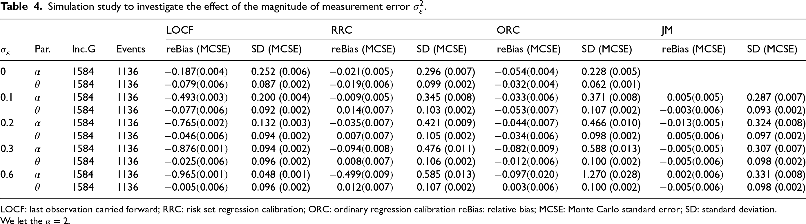
LOCF: last observation carried forward; RRC: risk set regression calibration; ORC: ordinary regression calibration reBias: relative bias; MCSE: Monte Carlo standard error; SD: standard deviation.
We let the
Parameter estimates assuming gamma frailty distribution and BMD as a longitudinal marker in the presence of delayed entry for only twin pairs (383 dizygotic twin pairs).
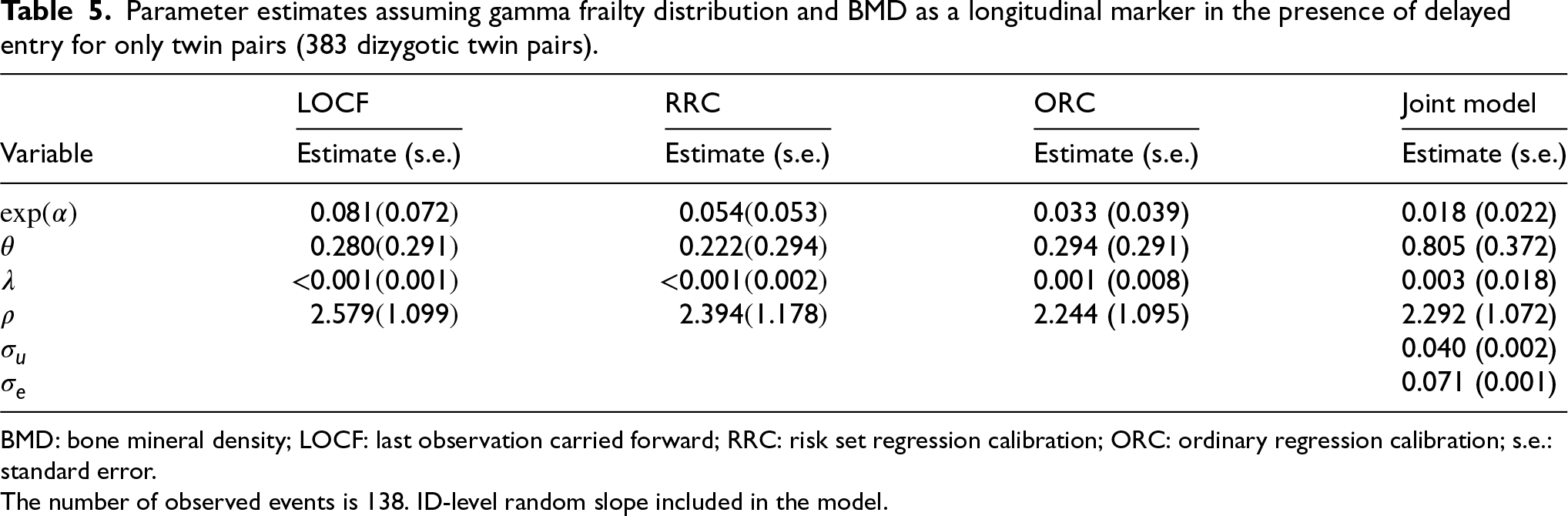
BMD: bone mineral density; LOCF: last observation carried forward; RRC: risk set regression calibration; ORC: ordinary regression calibration; s.e.: standard error.
The number of observed events is 138. ID-level random slope included in the model.
The simulations performed using Scenarios 1 and 2 assume that
We perform simulations to investigate the effect of the magnitude of measurement error
Tables 3 and 4, along with Tables 8 and 9 in the Appendix, present the performance of the proposed methods (LOCF, RRC, ORC, and JM) in estimating the parameters of the gamma shared frailty model under delayed entry, for various values of
When using the LOCF approach, the effect
The two regression calibration approaches yield similar results, except for cases of a large magnitude of
The JM approach performs well in estimating the effect
All the methods appear to estimate
Overall, the calibration and the JM approaches yield less bias in the estimation of parameters as compared to the LOCF approach in all considered scenarios. The bias in the estimation of
The joint model had convergence issues (about 10% of the simulated datasets do not yield standard error estimates of the parameter
Application: The effect of BMD on fracture incidence
We have access to longitudinal BMD observations and age at fractures of female dizygotic twins of 50 years of age and older from the TwinsUK (https://twinsuk.ac.uk). In Muli et al., 23 this dataset was analyzed using BMD as a time-fixed covariate to estimate the probability of a fracture in the next time period, that is, only the BMD at entry was used. BMD at entry appeared to be a statistically significant risk factor for fracture incidence. Here, we aim to estimate the relationship between BMD and fracture incidence over age. A joint model might be appropriate when there are genetic factors influencing both the BMD outcome over time and fracture incidence. On the other hand, the heritability of fracture incidence is lower, and identified genetic loci also have an effect on BMD, hence only a direct effect of BMD on fracture incidence might be biologically plausible as well. 27 Since the twins enter the study at different ages, we need to use the approaches developed in this paper. For all approaches, we consider a Weibull baseline hazard and gamma frailty distribution.
In this analysis, we consider BMD measurements after age 50 for the 766 individuals from 383 twin pairs (for results of the analysis of 383 twin pairs and 262 single twins see Table 12). For a sample of twins, their BMD profiles over age are given in Figure 2. We observe that indeed subjects enter the study at different ages and that for most subjects, BMD decreases with age. Furthermore, we notice that the time gaps between observed time points are quite large. The Kaplan–Meier curve taking into account delayed entry is depicted in Figure 3. It appeared that the probability of having a fracture before the age of 80 years is 0.3 to 0.4 in this cohort. Analysis of the longitudinal observed BMD showed that a model with a random intercept and slope at the individual level and a random intercept at the twin-level fitted the data well. All three random factors appeared to be statistically significant.
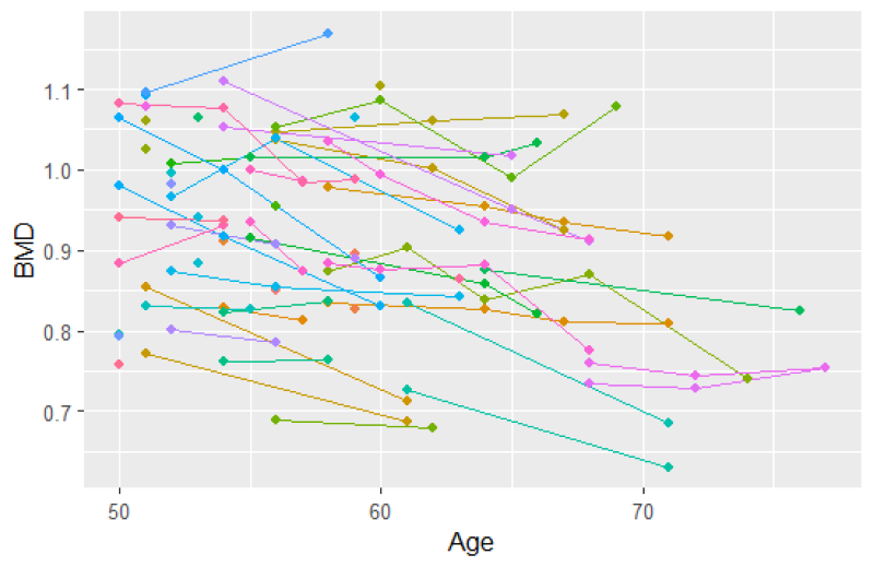
Spaghetti plot for 50 participants (a subset of the data).
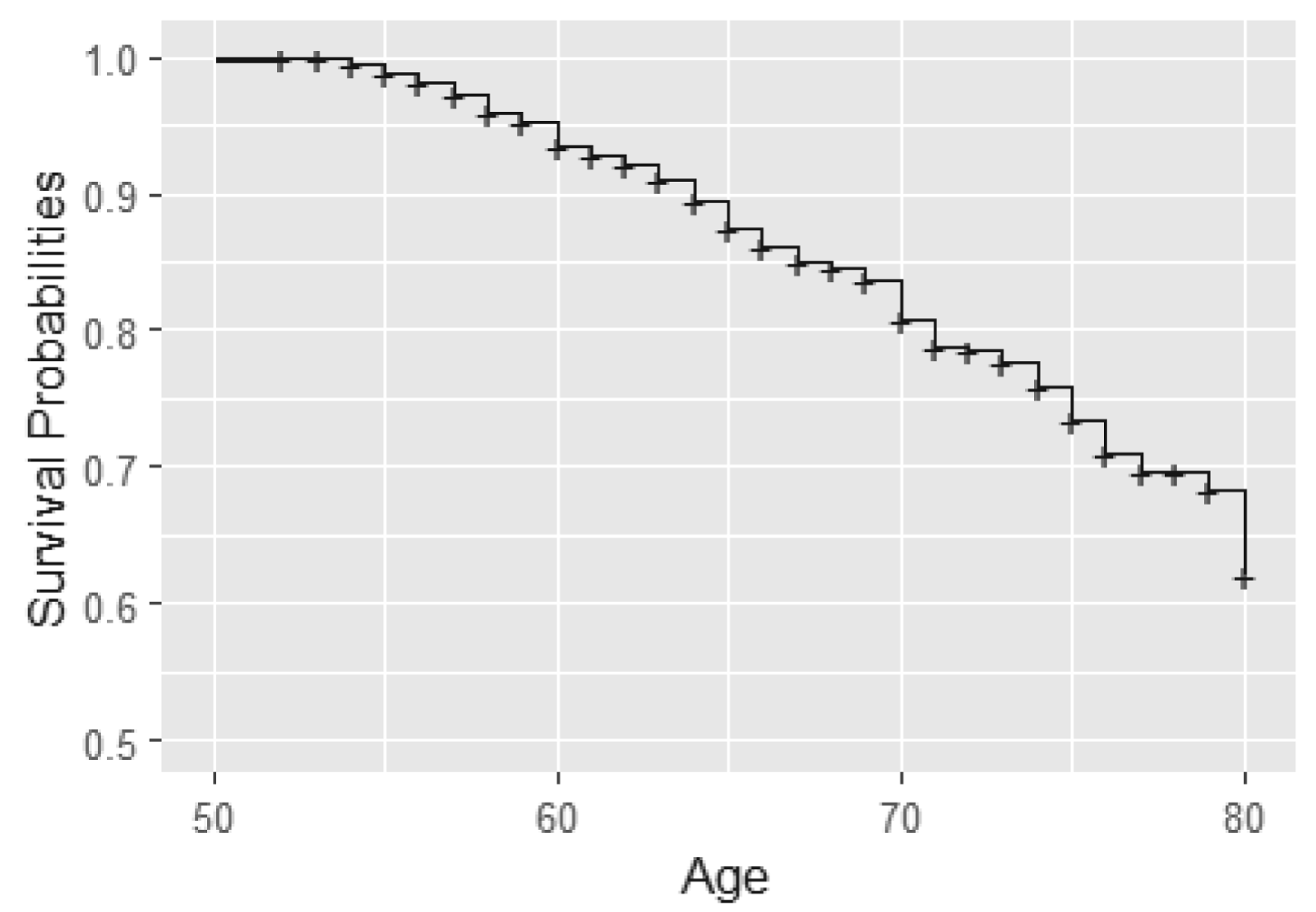
Kaplan–Meier curve for fractures using age as time scale.
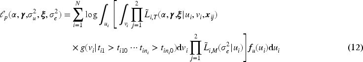
When modeling the BMD over time, we used mixed models including a random intercept and slope to model the correlation over time for a subject and a shared twin effect to model the correlation between twins. For ORC, we fit such a single mixed effects model in the first stage using all available data to compute predicted covariate values for each subject at each age in the sample. For RRC, we split the time into intervals: there are 30 unique ages at entry/event times (minimum age at entry is 50 years, minimum event time is 52 years, while the maximum event time is 85 years). For ages 51 and 52, we could only model a random twin effect, because individuals do not have repeated measurements at those time points. For the other unique age at entry/event times, the same mixed model as for ORC was used. From these models, we compute the predicted value of the covariate for individuals still at risk at a specific event time. For ORC and RRC, the data are arranged in start–stop format and the shared frailty model by maximizing the likelihood function (7). For the JM approach, we used the mixed model of the first step of ORC to obtain estimates of the fixed parameters and the empirical Bayes estimates of the random intercepts and slopes. Then, model (11) is fitted using the likelihood function (12).
All approaches gave a highly significant effect of BMD on fracture incidence (Table 5) (
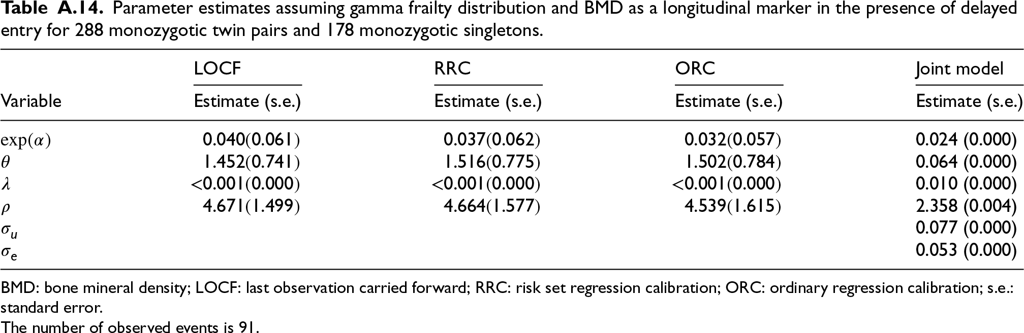
In a separate analysis, we model the effect of BMD on fracture incidence in the monozygotic dataset, using BMD measurements taken after age 50. This analysis includes 288 monozygotic twin pairs and 188 monozygotic single twins (see Tables 13 and 14 in the Appendix).
In this paper, we propose a novel joint model for a longitudinal marker and a survival outcome in twin studies. We developed four approaches (LOCF, ORC, RRC, and JM) to estimate the relationship between a longitudinal marker and a survival outcome, and the frailty variance using data from twins who enter the study at different ages. Through simulations, we showed that LOCF performs well for a dense grid of observed marker values. ORC, RCC, and JM also perform well for a sparse grid. When the measurement error is large (
Our novel JM approach can be interpreted as a hybrid approach in between a full joint modeling approach and the regression calibration approach. The advantage of a full JM approach is that it captures all variation that might be present in the data. Unfortunately, it is typically computationally infeasible to fit this model to the data. In contrast, our JM approach is computationally feasible, while regression calibration methods such as ORC and RRC are even more computationally efficient. Therefore, depending on the type of longitudinal marker, the density of the observations over time, and the magnitude of the measurement error, the calibration methods might be preferred. Specifically, in our simulation study, LOCF appears to perform well with small measurement error and dense grids, making it the standard method, as it is for singletons, for this scenario. ORC and RRC appear to be the preferred options for sparse grids with low measurement error. Low measurement error is a reasonable assumption in many practical settings. In studies in which rigorous data collection procedures are followed with standardized protocols, measurement error can be minimized. For example, in longitudinal studies measuring biomarkers such as blood glucose levels, where devices are regularly calibrated, the measurement error tends to be small. However, in studies with less controlled data collection processes, one should expect a larger measurement error, and in these cases, the joint model approach might be preferable. On the other hand, with a large measurement error, JM might show numerical instability. In such cases, ORC is an acceptable alternative.
The methods were applied to real data from the TwinUK twin registry. Here, LOCF yielded a weaker estimate than the other methods. Indeed, the gaps between the observed time points are quite large; hence, the two-stage approach should perform better. For the JM approach, the estimate of the variance of the frailty was larger than for the calibration methods. The differences between the estimates of the effect of BMD and of the frailty variance across the approaches are not statistically significant. The standard errors for the effect of BMD on survival are similar, although they slightly increase for the more advanced methods (ORC and JM). This can be expected, since the more advanced methods better capture the randomness in the longitudinal marker. For a full joint modeling approach, these standard errors might increase even further. Unfortunately, it appears computationally infeasible to apply this method to this dataset. However, given the small differences in standard errors between the methods used, a full JM approach would likely yield the same conclusion.
Our method is relevant for other survival outcomes and other twin studies beyond TwinsUK. Using age as an underlying time variable is often better interpretable than arbitrary follow-up time and results in more parsimonious models. For example, Cirulli et al. 1 modeled the effect of metabolome health on cardiovascular events in TwinsUK. They used follow-up as the underlying time variable and age-at-entry as covariate in a Cox proportional hazard model. For Danish twins, Tan et al. 2 modeled the effect of DNA methylation on mortality, adjusting for age at blood sampling. Also, when combining different studies in a meta-analysis, typically, follow-up times across studies are not comparable, and using age would be more appropriate. Our methods allow for the utilization of age as an underlying time scale, providing a more appropriate approach for analyzing longitudinal markers in twin studies. Furthermore, our proposed methods could be applied to other types of clustered survival data, such as paired data involving organs such as glycoma onset in eyes and hip replacement in hips due to osteoarthritis.
We proposed a novel two-stage approach for fitting a joint model as an alternative for a full joint estimation of all the parameters. We hypothesize that the computational complexity of a full-likelihood approach is often unfeasible in applications. Our two-stage joint model seems to represent a good tradeoff between complexity and applicability in the presence of measurement error. We have chosen to jointly model the cluster-specific parameters and the random error term of the longitudinal marker process and take the subject-specific random effects of the longitudinal marker process as independent of the time-to-event process. This assumption aligns with the idea that in twin studies, the shared unmeasured confounding between the biomarker and survival outcome is more likely to operate through the twin-level effect, rather than individual-specific effects, which justifies the focus on modeling
Several extensions of the methods can be considered, namely, modeling the recurrent fracture incidence and a more complex within-cluster structure to also include monozygotic twins. Additionally, we considered only complete twin pairs in our analysis, with results for including incomplete twin pairs provided in the Appendix. However, the likelihood function used is conditioned on both twins entering the study, which is violated when including single-twin members, as previously discussed in the context of time-fixed covariates. 28 Instead, one should condition on the entry of one twin, which complicates the likelihood function. Furthermore, to account for dropouts due to severe illness and death, competing risk models might be considered. Another extension is to use both the calendar and age scale simultaneously as proposed by Bower et al. 29 Lastly, we considered a Weibull baseline hazard in the simulation study and data application because it is commonly used as it is computationally attractive, and can take different shapes depending on the value of the shape parameter. It is straightforward to use more flexible baseline hazards, for example, by using splines. 30
In conclusion, the study of longitudinal markers in the presence of clustered survival data and delayed entry necessitates careful consideration of model choice. We have introduced a set of new models and estimation methods for this research area, along with specific recommendations based on the presumed underlying relationships, observation density, and error structures.
Footnotes
Funding
The authors disclosed receipt of the following financial support for the research, authorship, and/or publication of this article: This project has received funding from the European Union’s Horizon 2020 research and innovation programme, under H2020-MSCA-ITN grant agreement number 721815. TwinsUK is funded by the Wellcome Trust, Medical Research Council, European Union, Chronic Disease Research Foundation (CDRF), Zoe Global Ltd, and the National Institute for Health Research-funded BioResource, Clinical Research Facility and Biomedical Research Centre based at Guy’s and St Thomas’ NHS Foundation Trust in partnership with King’s College London.
Declaration of conflicting interests
The authors declared no potential conflicts of interest with respect to the research, authorship, and/or publication of this article.
Data and code availability statement
Data on information about fractures and BMD for the twins can be accessed through the TwinsUK data access committee. For information on access and how to apply, visit https://twinsuk.ac.uk. Code can be found on ![]() .
.
Appendix
Parameter estimates assuming gamma frailty distribution and BMD as a longitudinal marker in the presence of delayed entry for 288 monozygotic twin pairs and 178 monozygotic singletons.
| LOCF | RRC | ORC | Joint model | |
|---|---|---|---|---|
| Variable | Estimate (s.e.) | Estimate (s.e.) | Estimate (s.e.) | Estimate (s.e.) |
| 0.040 (0.061) | 0.037 (0.062) | 0.032 (0.057) | 0.024 (0.000) | |
| 1.452 (0.741) | 1.516 (0.775) | 1.502 (0.784) | 0.064 (0.000) | |
| <0.001 (0.000) | <0.001 (0.000) | <0.001 (0.000) | 0.010 (0.000) | |
| 4.671 (1.499) | 4.664 (1.577) | 4.539 (1.615) | 2.358 (0.004) | |
| 0.077 (0.000) | ||||
|
|
0.053 (0.000) |
BMD: bone mineral density; LOCF: last observation carried forward; RRC: risk set regression calibration; ORC: ordinary regression calibration; s.e.: standard error.
The number of observed events is 91.