
Abstract
Background
Clinical prediction models (CPMs) can be used to guide clinical decision making and facilitate conversations about risk between care providers and patients. 1 A CPM is a mathematical tool that takes patient and clinical information (predictors) as inputs and, most often, produces an estimated risk that a patient currently has (diagnostic model) or will develop (prognostic model) a condition of interest. 2 A common challenge in the development, validation and deployment of CPMs is the handling of missing data on predictors and outcome data. The most commonly used methods to handle missing data in CPM development and validation are complete case analysis or multiple imputation (MI) approaches,1,3 the latter of which is often heralded as the gold standard in handling missing data. Much of the past research around this topic has focused on the performance of different imputation methods to recover unbiased parameter estimates, for example, in causal inference or hypothesis testing.4–8 However, this topic has recently received renewed interest in the context of producing CPMs, with authors arguing the basis on which MI is commonly used relies too heavily on principles relevant to causal inference and descriptive research, which are less relevant when the goal is to provide accurate predictions. 9
Indeed, the objectives of prediction research differ from those of descriptive or causal inference studies. For the latter, missing data should be handled in such a way that minimises bias in the estimation of key parameters, and generally this is achieved through MI of missing data. In the development of prediction models, however, unbiased parameter estimates are not necessarily the ones that optimise predictive performance. 9 Moreover, in prediction research we must distinguish between handling missing data across the entire model pipeline; model development, model validation, and model deployment (or prediction time), and anticipate whether missing data shall be expected at deployment. Ideally, all predictors considered for inclusion in a CPM should be either readily available, or easily measured, at the point of prediction. There exist, however, notable examples that allow missingness at the point of prediction 3 ; the QRisk3 10 and QKidney 11 algorithms are examples of such models that allow users to make a prediction in the absence of clinical predictors (such as cholesterol) that may not be available, or easily measured, at the time of prediction.
Best practice states that the outcome should be used in the imputation model when applying MI, 12 creating a congenial imputation model. Clearly, the outcome is unknown at the prediction time, and applying imputation without the outcome would violate the assumption of congeniality. Since model validation should evaluate predictive performance under the same missing data handling strategy to be used in practice, the outcome should be omitted from any imputation model at validation, potentially resulting in less accurate imputations since predictors are normally predictive of the outcome. We, therefore, define ‘performance under no missingness’, where we assume all predictors are always available (or easily obtained) at deployment, and ‘performance under missingness’, assuming missing data is allowed and will be imputed at deployment.
Single imputation methods such as (single) regression imputation (RI) could provide a more pragmatic alternative to MI in the context of prediction. Here we use the term ‘regression imputation’ to refer to the form of single imputation that fits a regression model to impute missing values of missing predictors using observed data. The key difference between RI and MI is that RI is a deterministic process, that imputes the predicted value under the fitted imputation model (without error), whereas MI is a stochastic sampling process that can repeatedly sample from a distribution, incorporating the error associated with the fitted imputation model. It is important to note, however, that MI methods can also be underpinned by a regression model, but for illustrative purposes in this study we use the term ‘multiple imputation’ to refer to a method that produces multiple imputed datasets, and ‘regression imputation’ to one that imputes a single value for any missing predictors.
For RI to be applied in practice, only the imputation model(s) needs to be available alongside the full prediction model, as opposed to MI which generally also requires access to the development dataset. 13 Existing literature has, however, demonstrated several pitfalls of RI in the context of causal estimation – it is highly sensitive to model misspecification, can increase the correlation between predictors and underestimate variability in parameter estimates. 14 Although these issues may therefore persist within the prediction context, they may not apply since – as discussed above – the recovery of unbiased parameter estimates is no longer of direct concern. RI may also overcome some of the previously mentioned issues related to predictive modelling with MI since the inclusion of the outcome in the imputation model is not recommended. 1 To our knowledge these issues and challenges have not been studied to date.
Both MI and RI are techniques devised under the assumption that data are missing at random, that is, missingness does not depend on unobserved values. The validity of the MAR assumption within health data is often dubious, especially when using routinely collected data,15,16 however these definitions were created with the goal of recovering unbiased parameter estimates in mind and therefore may be less relevant to the prediction modelling context. 9 Within routinely collected data, the recording of key clinical markers is often driven by the needs of the patient and the clinical judgments of the care provider. 16 Missingness is therefore potentially informative with respect to a patient's current or future condition, and including information about the way an individual has been observed in a prediction model has the potential to improve its predictive performance. 17 A commonly used, effective approach to achieve this is through the inclusion of missing indicators as predictors in a CPM.
This study, therefore, aims to explore the use of missing indicators as model predictors alongside both RI and MI. We explore the effect of omitting/including the outcome from each imputation model at development and imputing data without the outcome at validation (and therefore deployment). We compare the two imputation strategies when missingness is both allowed and prohibited at the point of prediction. Our results will inform recommendations on the handling of missing data during model development and deployment that will be especially relevant to applied researchers developing clinical prediction models.
Methods
We performed an extensive simulation study in which we evaluated a range of different missingness mechanisms. Our study has been designed according to best practice and reported according to the ADEMP structure (modified as appropriate for a prediction-focused study), proposed by Morris et al. 18 We also applied the methods to a real-world critical care dataset. In this section, we first describe the methods of the simulation study before describing the empirical study methods in Section 2.8.
Aims
The primary aim of this study is to compare MI and RI approaches in imputing missing data when the primary goal is in developing and deploying a prediction model, under a range of missing data mechanisms (Missing Completely at Random (MCAR), Missing at Random (MAR) Missing Not at Random (MNAR)), with/without a missing indicator and with/without the outcome included in the imputation model. Each of these will be examined both allowing for and prohibiting missing data at deployment, and performance will be estimated separately for each of these two scenarios.
Throughout this study, we assume that both the missingness mechanism and handling strategy will remain the same across validation and deployment, and therefore validation is a valid replication of model deployment and our performance estimates are reliable estimates of model performance at deployment. The only case where this is not true is when we impute data using the outcome at validation, which will be discussed in more detail in the following sections.
Data-generating mechanisms
We focus on a logistic regression-based CPM to predict a binary outcome, Y, that is assumed to be observed for all individuals (i.e. no missingness in the outcome) during the development and validation of the model. Without loss of generality, we assume that the data-generating model contains up to three predictors,
We construct four separate DAGs depicted in Figure 1, each representing different missingness structures covering: MCAR, MAR, MNAR dependent on
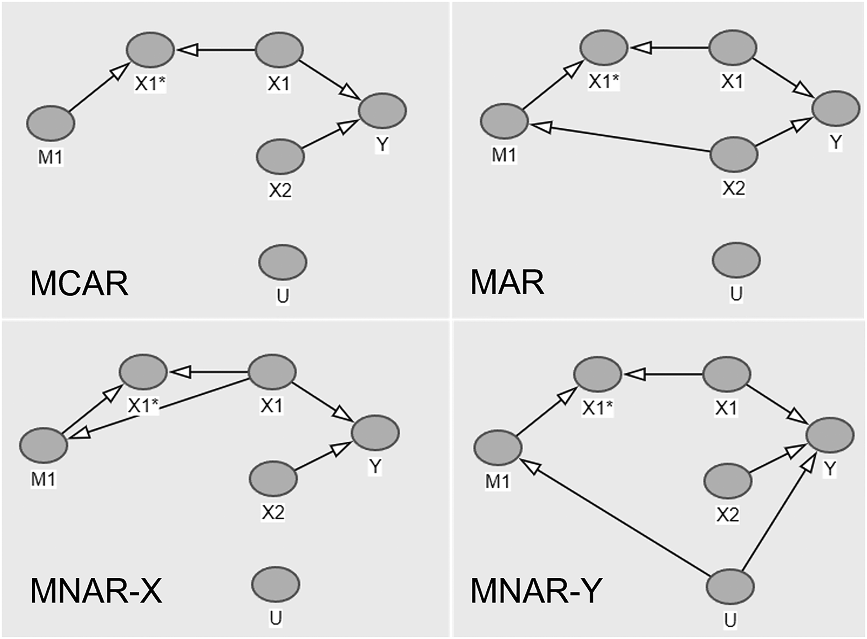
Directed acyclic graphs for four missingness structures.
The DAGs further illustrate how missingness in
In order to reconstruct these DAGs in simulated data, we stipulate the following parameter configurations:
where

and
The parameter values above were selected to represent what might be observed in real-world data, assuming that
Datasets were generated with
We further vary the available sample size
We fit the models on the development data and calculate performance measures on the derived models applied to the validation set. The full simulation procedure is illustrated in Figure 2. Note that in this instance, we fit the imputation models separately in the development and validation sets. Since the DGMs and missingness mechanisms remain constant between the two datasets, we assume that the fitted imputation model would not change and this is therefore a valid approach to take. In a real-world setting, however, this would not be feasible as only a single patient's data would be available at the point of prediction, and we would want to use the same imputation model as was used/developed in the development data. We explore this further by adopting a different strategy in the real data example (Section 3.8).
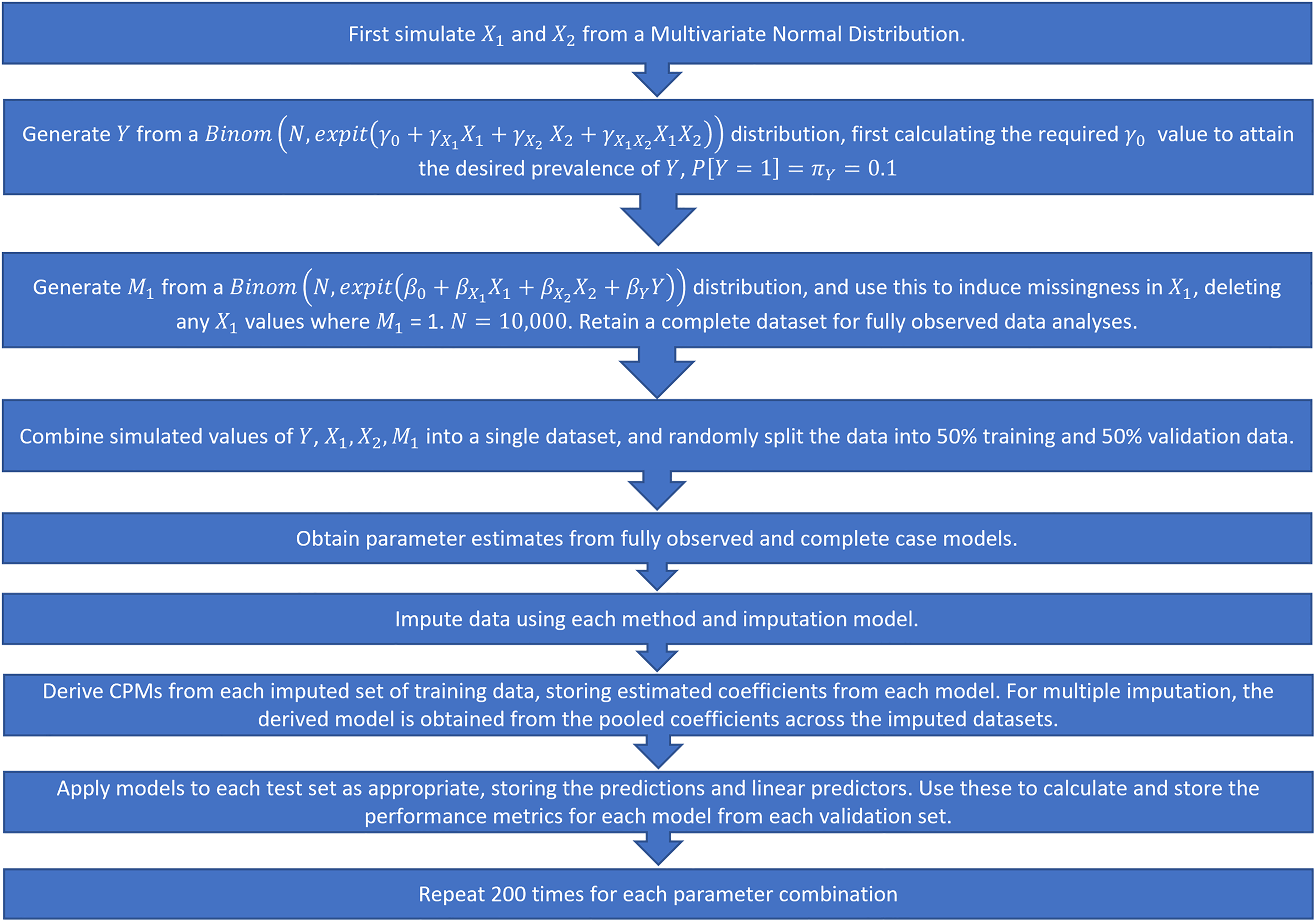
Simulation procedure, step-by-step.
Each simulated DGM was repeated for 200 iterations. The parameter values listed above result in a total of 864 parameter configurations. A total of 200 iterations was selected as optimal to balance the requirement to obtain reliable estimates of key performance metrics (by using a sufficient number of repetitions) with the size of the study and computational requirements of repeatedly running MI over a large number of simulated scenarios.
We consider two main methods for handling missing data at the development and deployment stages of the CPM pipeline: MI and RI. MI can be applied with relative ease at the model development stage, specifying an imputation model and method for every predictor with missing data (in this case just
Applying MI to incomplete data for new individuals at deployment is more challenging as it is not generally possible to extract the final imputation model from the output provided by standard statistical software. In order to ‘fix’ the imputation model for new individuals, it has therefore instead been proposed that the new individual's data should first be appended to the original (imputed) development data, and the imputation re-run on the new stacked dataset.13,22,23 RI, on the other hand, is easier to implement at the point of prediction, since models can be defined for each (potentially) missing predictor, and these models can be stored (alongside the actual CPM) and used to impute at deployment for new individuals. Ideally, model validation should follow the same steps as model deployment in order to properly quantify how the model will perform in practice. 3 However, since validation is usually completed for a large cohort of individuals at once (as opposed to a single individual), it is likely that missing data imputation would take place as a completely separate exercise, with the imputation model depending solely on the validation data.
Fitted CPMs
We fit three possible CPMs to the development data (under each different imputation method), firstly with a simple model including both derived predictors and their interaction. We then fit models incorporating missing indicators, as well as considering a model with an interaction between the missing covariate Predictors and their interaction only: Inclusion of an additional missing indicator: Inclusion of an interaction between the
Each model was developed using completed datasets derived under MI and RI, with and without the outcome in the imputation model. The derived models were then applied to the validation set according to the strategies listed in Table 1.
Imputation and validation strategies.
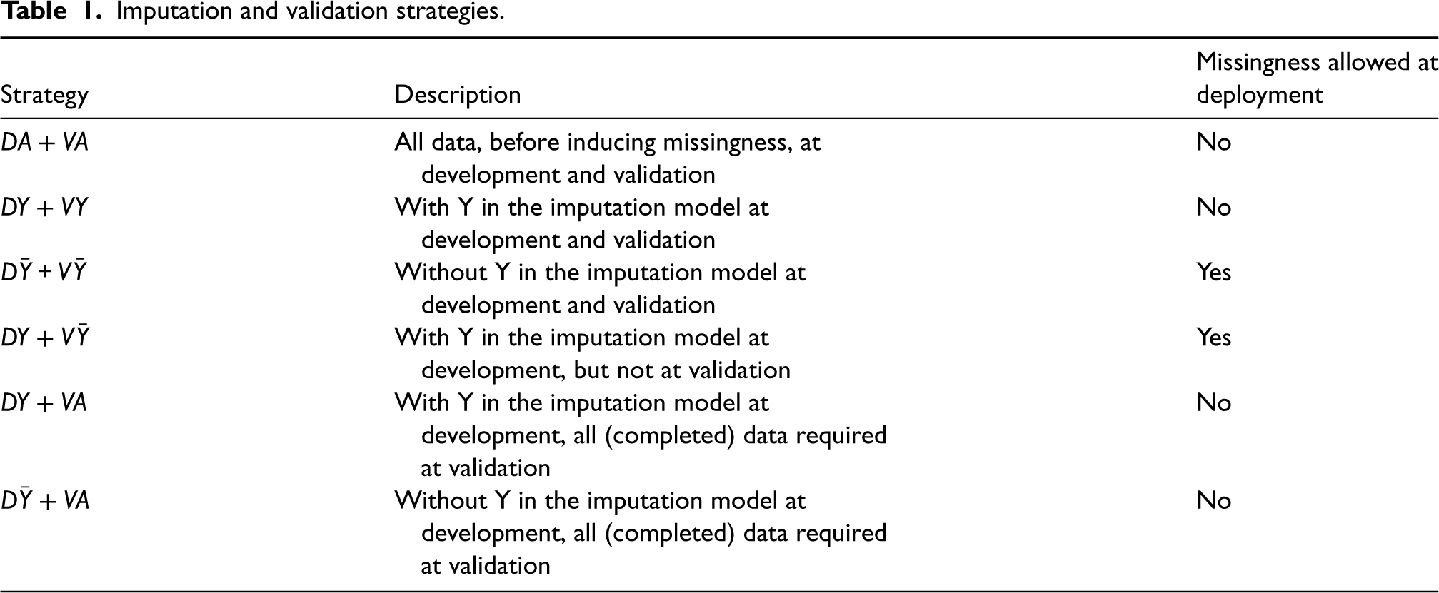
Imputation and validation strategies.
We apply each of the imputation and validation strategies described in Table 1,
Parameter estimates were pooled across the imputed datasets according to Rubin's rules, and, similarly, we took the ‘pooled performance’ approach to validation whereby imputation-specific predictions are obtained in the multiply imputed validation datasets, the predictive performance of each imputed dataset is calculated, and then these estimates of model performance are pooled across the imputed datasets. 25
The fully observed data strategy in
In strategies
Target and performance measures
Our key target is an individual's predicted risk, and we compare each method's ability to estimate this using the following metrics of predictive performance, covering both calibration and discrimination1,26:
Calibration-in-the-large (CITL) – the intercept from a logistic regression model fitted to the observed outcome with the linear predictor as an offset. Calibration slope – the model coefficient of the linear predictor from a model fitted to the observed outcome with the linear predictor as the only explanatory variable. Discrimination (Concordance/C-statistic) – a measure of the discriminative ability of the fitted model. Defined as the probability that a randomly selected individual who experienced the outcome has a higher predicted probability than a patient that did not experience the outcome. Brier score – a measure of overall predictive accuracy, equivalent to the mean squared error of predicted probabilities.
We assume that the estimates of the above measures are valid representations of performance at model deployment, based on the following assumptions: (1) when missingness is allowed at deployment, it will be imputed in the same way as performed in our validation set, (2) the missingness mechanism will not change between validation and deployment, and (3) when missingness is not allowed at deployment, we assume that the data-generating mechanism remains constant across validation and deployment.
We also extract the obtained parameter estimates and any associated bias from each fitted CPM.
Software
All analyses were performed using R version 3.6.0 or greater. 27 The pROC library 28 was used to calculate C-statistics and the mice package 29 was used for all imputations. Code to replicate the simulation can be found in the following GitHub repository: https://github.com/rosesisk/regrImpSim.
Application to MIMIC-III data
Data
To illustrate the proposed missing data handling strategies, we applied the methods studied through the simulation to the Medical Information Mart for Intensive Care III (MIMIC-III) dataset. 30 MIMIC-III contains information on over 60,000 critical care admissions to the Beth Israel Deaconess Medical Center in Boston, Massachusetts from 2001 to 2012.
Prediction model: predictors, outcome and cohort
We develop, apply and validate a CPM in the MIMIC-III data based on the set of predictors used in the qSOFA score, 31 a CPM used to predict in-hospital mortality in patients with suspected sepsis. Bilirubin is included as an additional model predictor since the qSOFA predictors are likely to be completely observed for the majority of patients and would therefore not allow a proper illustration of our proposed methods. Bilirubin is included in other commonly-used critical care mortality scores such as SAPS III 32 and MODS. 33 Additionally, we include age and gender in the model as these are always observed in the example dataset and often provide prognostic information.
Data for the clinical predictors was taken from the first 24 h of each patient's critical care stay, and therefore the cohort is restricted to only patients with a stay of at least one full day, and only a single stay was used for each patient. Where repeated predictor measurements are made over the first 24 h, the maximum is taken for respiratory rate and the minimum for systolic blood pressure and Glasgow Coma Scale. All numeric predictors (age, respiration rate, systolic blood pressure, Glasgow Coma Scale and serum bilirubin) are entered into the model in their original forms. For each missingness strategy, the same three CPMs were fit and evaluated as in the simulation: main effects only (
Imputation strategies
In the simulation part of this paper, RI is applied using the mice package in R under the ‘norm.predict’ method. This method, however, can only be used in the case of a single missing predictor. For the real data application, therefore, we will manually derive the underlying imputation models (in the development data) and use these to impute the missing predictors in both the development and test sets.
RI models were derived within the subset of patients that the model will be used within. For example, the imputation model used to impute GCS using age, gender and systolic blood pressure will only be derived in patients that have missing bilirubin and respiratory rate, as it will only be applied to patients with this observed missingness pattern. Where the sample size is insufficient in the target missingness-pattern cohort, data from complete cases were instead used to develop the imputation model.
13
The minimum required sample size required for the development of each imputation model is
In the simulation part of this study, MI is run independently in the development and test sets. Clearly, this is not feasible at the point of prediction with real data as only a single new observation is available at a time. Incomplete data from the MIMIC-III dataset was therefore stacked on top of (multiply) imputed development datasets on a patient-by-patient basis, therefore fixing the imputation model used during development. This process is illustrated in Appendix 5 of the Supplemental Materials. To mimic a real-world deployment, the outcome was set to missing in the appended test patient data and (where necessary) this was imputed and used to inform imputations for the remaining missing predictors (under a new strategy,
Due to the described differences in the way MI was run between the simulated data and the real-data example, results are presented in the Supplemental Materials for an equivalent ‘independent MI’ run in the MIMIC-III data for comparison.
Model validation
A split-sample approach to validation in the MIMIC-III data was taken, using a random 70%/30% development/validation split. The same four performance metrics were evaluated in the empirical test data as in the simulation study.
Results: simulation
In this section, we report the results of the simulation study. Select parameter combinations have been chosen to highlight important results here, but full results for all combinations are made available in a rShiny dashboard at https://rosesisk.shinyapps.io/regrimpsim.
Predictive performance
Figure 3 summarises the estimated Brier Scores for each strategy defined in Table 1 for both imputation methods and all fitted outcome models, and calibration slopes are presented in Figure 4. The imputation strategies have been split according to whether or not they allow missingness at model deployment.
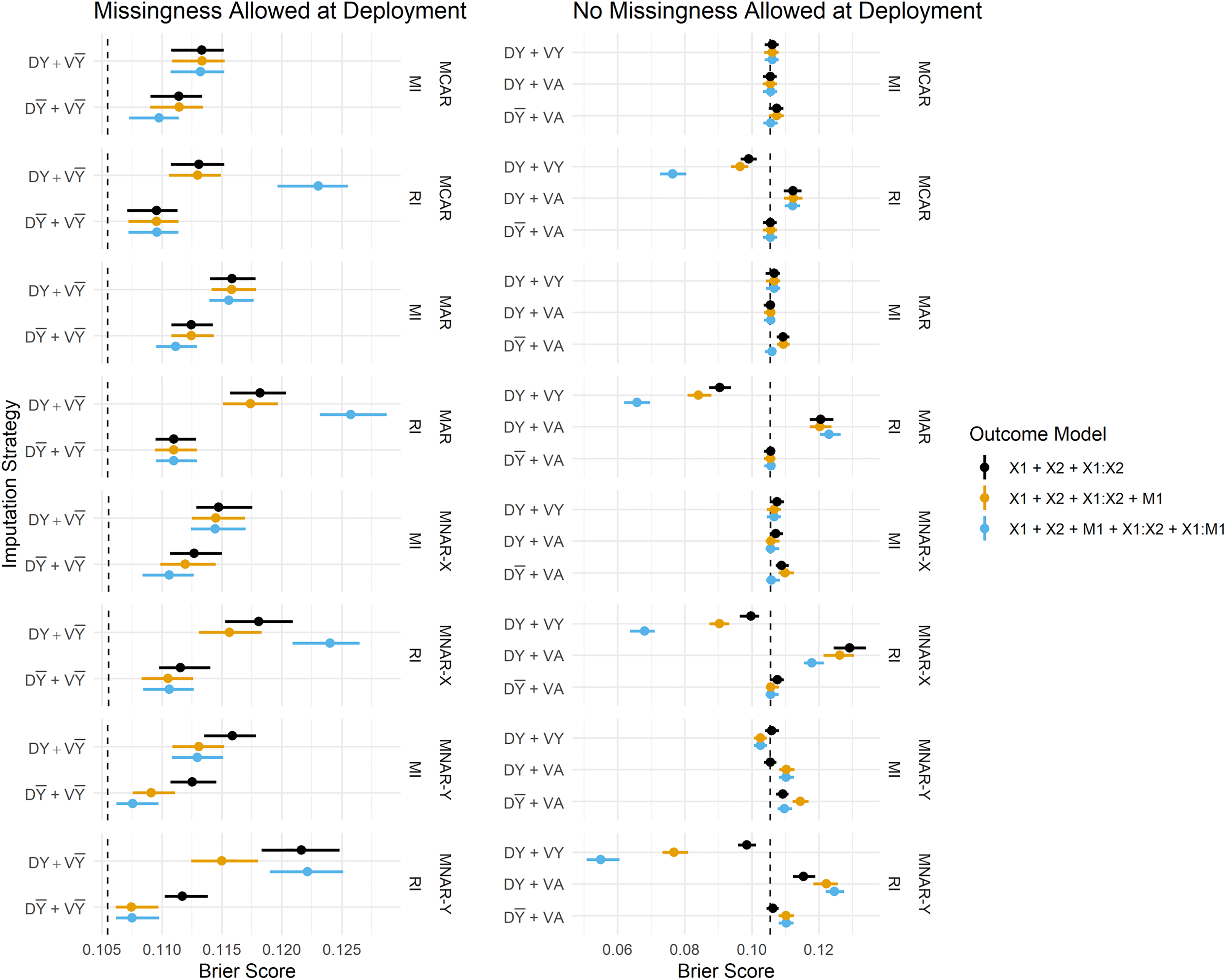
Brier Score estimates across development/validation scenarios, imputation methods and missingness mechanisms. The vertical dashed lines represent estimates from the complete data scenario (DA + VA). DY = Y included in the imputation model at development, D
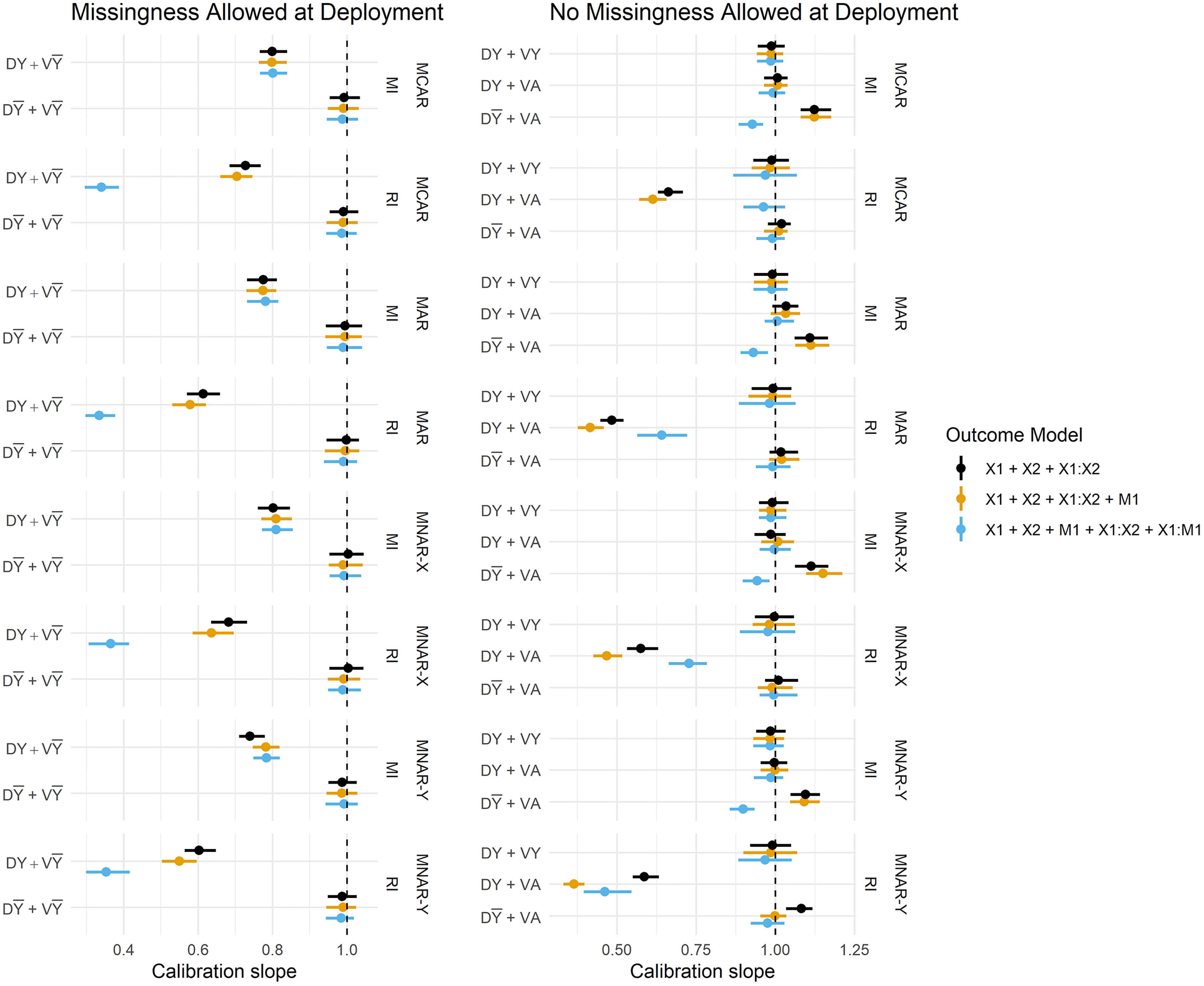
Calibration slope estimates across imputation strategies, imputation methods and missingness mechanisms. Vertical dashed lines are placed at 1. DY = Y included in the imputation model at development, D
For simplicity, we restrict our results to a single parameter configuration for each missingness mechanism. The following parameters remain fixed throughout this section:
When missingness is allowed at deployment (i.e. imputation will be applied at the point of prediction), we primarily want to know whether imputation should be performed with or without the outcome at development, since at deployment it must be omitted from the imputation model (by definition). We observe that predictions in the validation set are far better calibrated under
When complete data is required at deployment, RI still performs better under
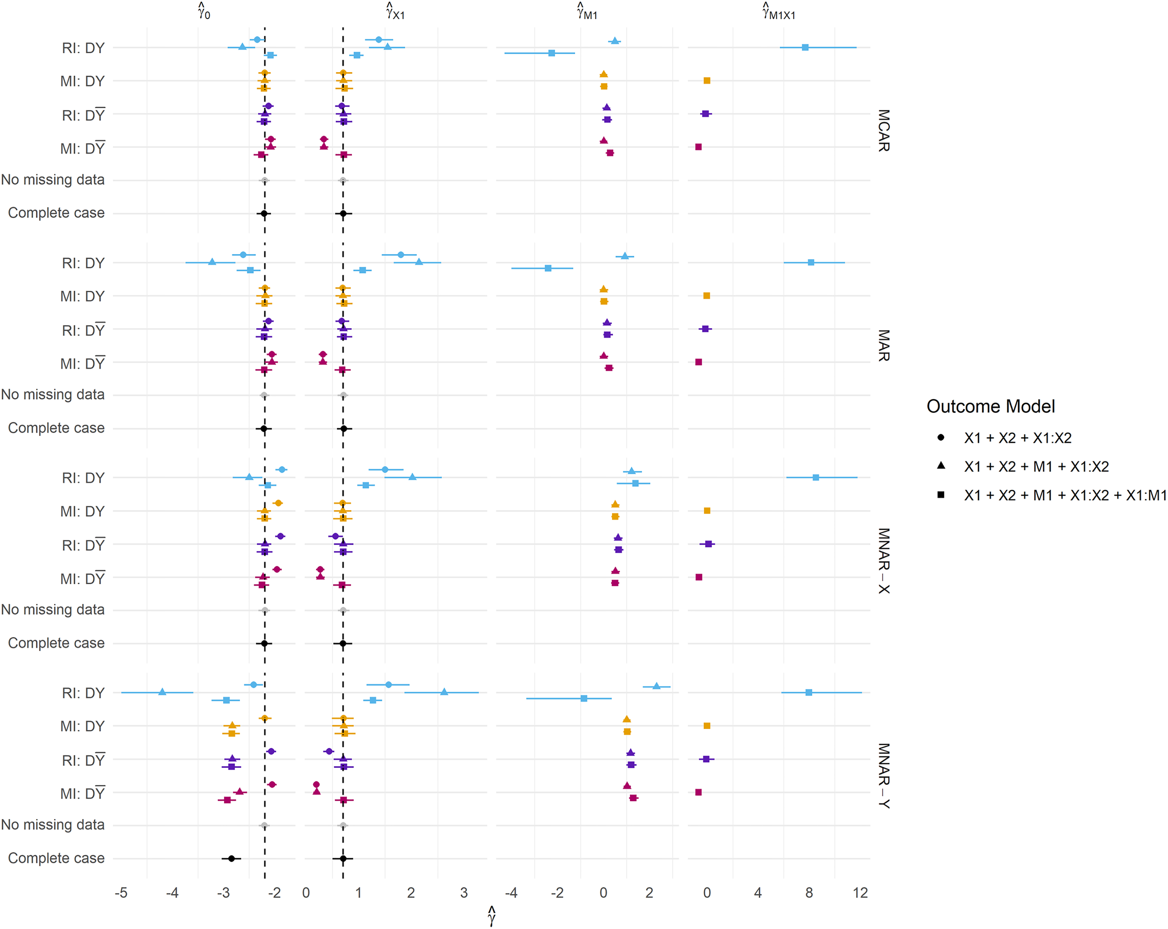
Parameter estimates across all missingness mechanisms. Missingness is fixed at 50%. DY = Y included in the imputation model at development, D
A notable result is that the
Overall, the performance estimates from MI are more stable than those from RI; the differences in Brier Score between the various imputation strategies (e.g.
Inclusion of a missing indicator
The inclusion of a missing indicator appears to have minimal impact on the Brier Score and calibration under most methods and imputation strategies, with a few notable exceptions.
Missingness allowed at deployment
Under MNAR mechanisms and missingness allowed at deployment, the inclusion of a missing indicator in the outcome model provides reductions in the Brier Score, and considerable improvements in the C-statistic (under MNAR-Y for both imputation methods, C-statistics presented in Appendix 2 of the Supplemental Materials).
The inclusion of a missing indicator and its interaction with
No missingness allowed at deployment
Inclusion of the indicator corrects the CITL for both MI:
Interestingly, the inclusion of the
Sample size
For the scenarios presented in this section, simulations were repeated, varying the sample size across 500, 1000, 5000 and 10,000. Visualisations of these results are presented in Appendix 4 of the Supplemental Materials. As expected, estimates of model performance were far more unstable at smaller sample sizes (< 5000), and model calibration improved as the sample size increased. There is some evidence of overfitting at smaller sample sizes, which is more pronounced in the models including missing indicators and their interactions than main effects alone.
Parameter estimation
We further present results for the CPM parameter estimates for selected scenarios presented in Figure 5. The same parameter configurations as specified in previous sections are used here.
Presented are the coefficients obtained from fitting each model within the development data. For MI, we present coefficients pooled according to Rubin's rules.
RI using the outcome in the imputation model consistently produces parameter estimates that are both biased and much larger in magnitude than any other method, and this is reflected in the predictive performance estimates. We frequently observe Brier Scores (Figure 3) that are too extreme under
Perhaps as expected, MI:
Results: MIMIC-III data example
A total of 33,306 patients were included in the analysis of the MIMIC-III data. A total of 23,314 were randomly assigned to the development set, and the outcome prevalence in the development cohort was 2610/23,314 = 11.2%. The remaining 9992 patients formed the validation set, and had an outcome prevalence of 1084/8908 = 10.8%. A total of 14,474 patients had complete data in all predictors. 18,713 patients were missing bilirubin, 424 were missing Glasgow Coma Scale, 447 missing respiratory rate and 439 missing systolic blood pressure. A total of 10 different missingness patterns were observed (where complete cases are classed as a missingness pattern) resulting in 17 derived (regression) imputation models. Given the six model predictors, the minimum required sample size for the development of the imputation models was
Since the MIMIC-III data contains missing data in the predictors, the two imputation/validation strategies dependent on complete predictor information at deployment (
Estimates of the predictive performance of the fitted CPMs applied to the MIMIC-III data under each imputation strategy and development/validation scenario are presented in Figure 6. The magnitude of difference in the performance metrics between methods and scenarios was generally smaller than in the simulation study, but some key findings remain. Summaries of all predictive performance measures, and differences between MI and RI, and omitting/including the outcome in the imputation model are presented in the Supplemental Materials in Appendices 7 to 9, respectively.
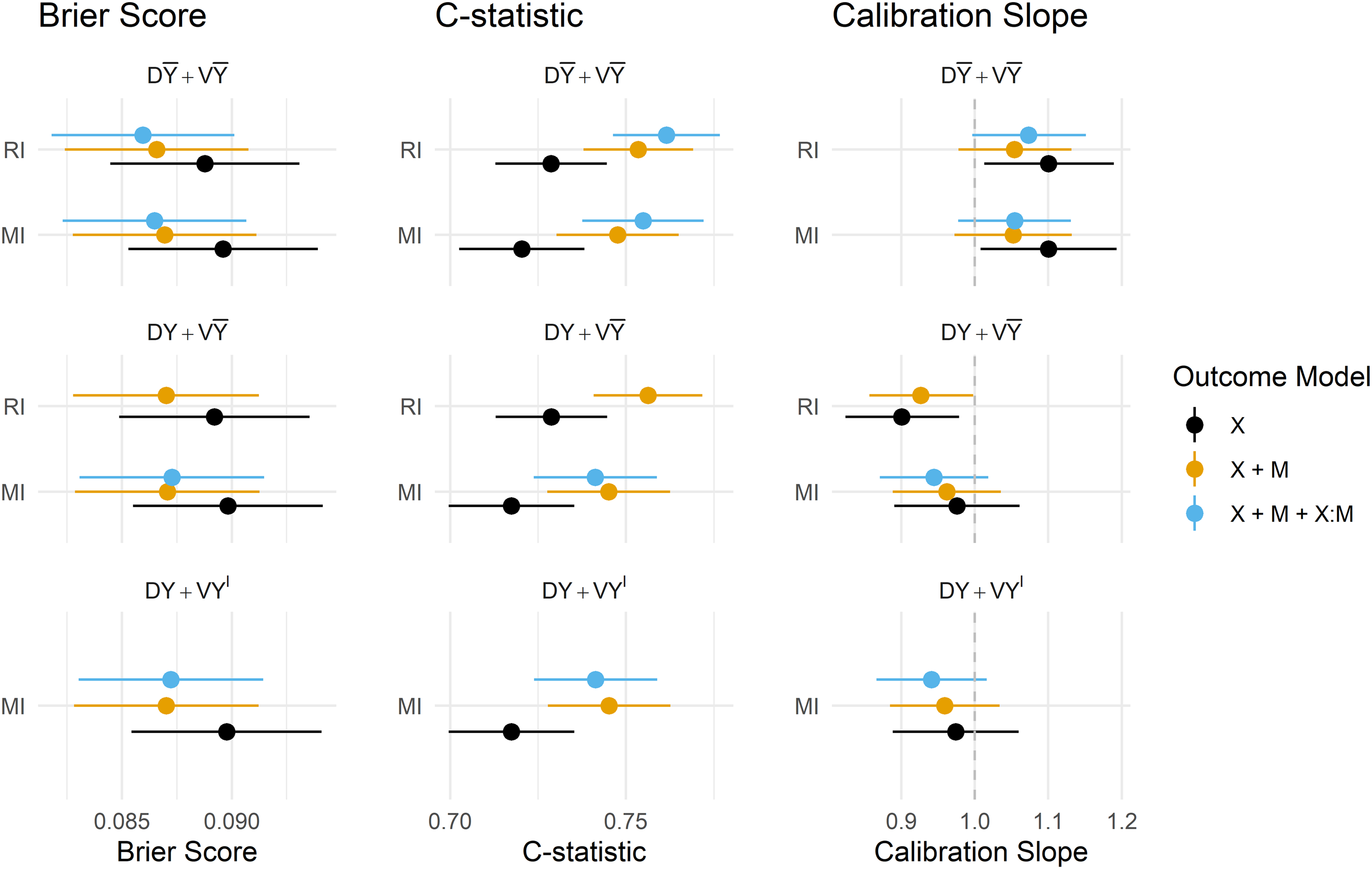
Predictive performance of imputation methods, model forms and imputation/validation strategies. DY = Y included in the imputation model at development, D
Under RI, omitting the outcome from the imputation model was again preferred in terms of model calibration, though in the MIMIC-III data, there was practically no difference in overall accuracy or model discrimination from including the outcome. Attempting to fit a CPM on data that uses the outcome to impute missing predictors, and also contains interactions between predictors and their missing indicators failed: models did not converge and resulted in extreme estimates of the model coefficients, and results for this outcome model under
MI performed similarly under
The inclusion of missing indicators (and their interaction) mitigated the under/overfitting slightly for both RI and MI, and offered minor improvements in discrimination, Brier Score and calibration for both methods under
Predictions obtained via both the
Discussion
In this study, we have assessed model performance for MI and RI, with and without the use of missing indicators across a range of missingness mechanisms across simulated and real data. We considered how/when the outcome should be used in the imputation model for missing covariates, whether RI could offer a more practical and easier-to-implement solution than MI, and how the inclusion of missing indicators affects model predictive performance. All of these questions were considered in relation to whether or not missing data will be allowed once the model is deployed in practice. We have provided a concise list of recommendations in Table 2.
Table of recommendations for the use of multiple imputation, regression imputation and missing indicators in the development and deployment of clinical prediction models.
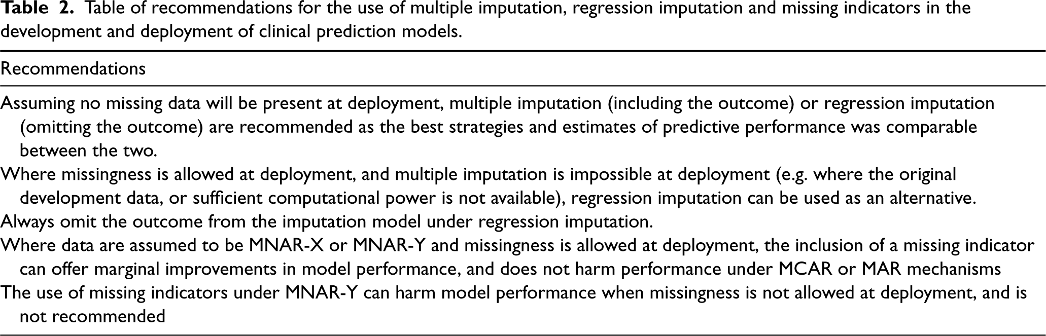
Table of recommendations for the use of multiple imputation, regression imputation and missing indicators in the development and deployment of clinical prediction models.
In the context of recovering unbiased parameter estimates, the literature advocates the use of the observed outcome in the imputation model for MI. 12 In the context of predictive performance, we found that RI consistently performed better when Y is instead omitted from the imputation. This strategy is recommended by Steyerberg 34 for RI, where the author notes that including the outcome in the imputation model artificially strengthens the relationship between the predictors and outcome. MI overcomes this issue by introducing an element of randomness to the imputation procedure.
We further observed that the performance of a model with inconsistent imputation models between the development and validation stages (
A related issue lies in the inclusion of additional variables in the imputation model that are not model predictors. This could arise in external validation studies where missingness occurs in the predictors, and additional information is available and used to impute them. Although this was not directly covered by the study, we anticipate that the resulting inconsistency in imputation models between model development and validation could negatively impact the model performance since we observed that performance was strongest when imputation models remained consistent across development, validation and deployment. It is therefore worth considering (at the time of model development) which variables should be used in imputation models, and whether these are likely to be available in future validation and deployment scenarios.
We have demonstrated that RI could offer a practical alternative to MI within the context of prediction. Estimates of predictive performance were practically indistinguishable between RI and MI when the preferred imputation model was applied in both simulated and real data settings. As discussed above, there are several challenges associated with applying MI during the deployment of a CPM, including but not limited to requiring access to the development data and the availability of computational power and time. Recent developments have, however, proposed methods that potentially mitigate these requirements. 23 RI also overcomes both of these major issues, in that only the deterministic imputation models would be required to produce imputations during model deployment. We emphasize, however, that RI consistently showed extremely poor performance when the observed outcome was included in the imputation model, and this method should therefore only be used when missing model covariates are imputed using observed covariates. MI, on the other hand, proved to be more stable across a range of scenarios and imputation models.
The careful use of missing indicators has also proven to be beneficial in specific cases. For example, under MNAR-X, MI has marginally stronger performance in both imputed and complete deployment data when a missing indicator is included in the outcome model. Under incomplete data at deployment, the inclusion of an indicator further provided small improvements in overall predictive accuracy to both methods under MNAR-Y. Since MI is only assumed to recover unbiased effects under MAR, the indicator appears to correct this bias under informative missingness patterns. However, we noted some surprising results in the use of indicators when data are MNAR-Y; specifically, when missing data are not allowed at deployment the inclusion of the indicator is harmful and resulted in small increases in the Brier Score, and poor Calibration-in-the-large. In our real data example, the inclusion of a missing indicator offered improvements in model discrimination, calibration and overall accuracy under the preferred strategy, omitting the outcome from the imputation at all stages of the model pipeline.
Related literature under a causal inference framework by Sperrin et al. 9 and Groenwold et al. 35 has found that the inclusion of missing indicators is not recommended under MCAR, and can lead to biased parameter estimates under this missingness structure. van Smeden et al. 36 discuss at length how missing indicators should be approached with caution in predictive modelling – inclusion of a missing indicator introduces an additional assumption that the missingness mechanism remains stable across the CPM pipeline; an assumption that is generally dubious, but especially within routinely collected health data. The propensity to measure certain predictors is likely to vary across care providers, settings and over time as clinical guidelines and practices change. This in turn potentially changes the relationship between the missing indicator and the outcome and could have implications for model performance. As others have highlighted, the strategy to handle missing data should be devised on an individual study basis, taking into consideration the potential drivers of missingness, how stable these are likely to be, and how/whether missing data will be handled once the model has been deployed.
We recommend that the strategy for handling missing data during model validation should mimic that to be used once the model is deployed, and that measures of predictive performance be computed in either complete or imputed data depending on whether missingness will be allowed in the anticipated deployment setting or not. For example, complex model applications integrated into electronic health record systems are better suited to applying imputation strategies at the point of prediction, whereas simple models that require manual data entry at the point-of-care are more likely to require a complete set of predictors. The difference between performance allowing for and prohibiting missing data at deployment may also be of interest in assessing any drop in performance related to the handling of missing data. Interestingly, we have observed somewhat different results depending on whether missingness is allowed at deployment or not. It may therefore be preferable to optimize a model for either one of these use cases, resulting in a different model (and hence different coefficients) dependent on whether we envisage complete data at deployment. Ideally, any model predictor considered for inclusion in a CPM should be either routinely available or easily measured at deployment. There are, however, several existing use cases where important predictors can be missing both at model development and deployment (e.g. QRisk3 10 ) and we envisage that models integrated directly into existing clinical systems would be required to make predictions in the absence of some predictor information. We expect that the findings of this work are especially relevant to such use cases.
Although we have considered a wide range of simulated scenarios, a key limitation to this study is that we only considered a relatively simple CPM with two covariates, where only one was allowed to be missing. This was to restrict the complexity and size of the work, as only a limited set of scenarios can realistically be presented. We do, however, expect that the fundamental findings would generalise to more complex models (as was found in the MIMIC-III example) since we could consider each of the two model predictors to represent some summary of multiple missing and observed predictors. With more predictors in the model, there would not be any additional missingness mechanisms and we, therefore, anticipate that such complex models would not provide any additional insight. A further possible limitation is that this work has been restricted to the study of a single binary outcome, although we would not expect the results to change in the context of e.g., continuous or time-to-event outcomes. We accompany this work with a rShiny dashboard allowing readers to explore our results in more detail across the entire range of parameter configurations. Finally, we did not consider uncertainty in individual-level predictions as a measure of predictive performance. Typically, only point estimates of individual-level risk are provided during the deployment of a clinical prediction model so we focused on measures of predictive performance that validate these point estimates (i.e. calibration and discrimination). However, it is posssible that differences would be observed in the precision and coverage of prediction intervals, 37 or the stability of the individual-level predictions derived under RI and MI.38,39
Avenues for further work would include exploring the impact of more complex patterns of missingness in multiple predictor variables. As the number of incomplete predictors increases, so does the number of potential missing indicators eligible for inclusion in the outcome model, which could introduce issues of overfitting,40,41 and variable selection becomes challenging. Here we have also limited our studies to scenarios where the missingness mechanism remains constant between development and deployment, however, it would be interesting to explore whether these same results hold if the mechanism were to change between the two stages, or indeed if different missing data handling strategies were to be used across different stages of the model pipeline.
We have conducted an extensive simulation study and real data example, and found that when no missingness is allowed at deployment, existing guidelines on how to impute missing data at the development are generally appropriate. However, if missingness is to be allowed when the model is deployed into practice, the missing data handling strategy at each stage should be more carefully considered, and we found that omitting the outcome from the imputation model at all stages was optimal in terms of predictive performance.
We have found that RI performs at least as well as MI when the outcome is omitted from the imputation model, but tends to result in more unstable estimates of predictive performance. Missing indicators can offer marginal improvements in predictive performance under MAR and MNAR-X structures, but can harm model performance under MNAR-Y. We emphasise that this work assumes that both the missingness mechanism and missing data handling strategies remain constant across model development and deployment, and the performance of the proposed approaches could vary when this assumption is violated.
We recommend that if missing data is likely to occur both during the development and deployment of a CPM, that RI be considered as a more practical alternative to MI, and that if either imputation method is to be applied at deployment, the outcome be omitted from the imputation model at both stages. Model performance should be assessed in such a way that reflects how missing data will occur and be handled at deployment, as the most appropriate strategy may depend on whether missingness will be allowed once the model is applied in practice. We also advocate for the careful use of missing indicators in the outcome model if MNAR-X can safely be assumed, but this should be assessed on a study-by-study basis since the inclusion of missing indicators also has the potential to reduce predictive performance, especially when missingness is not permitted at deployment.
Supplemental Material
sj-docx-1-smm-10.1177_09622802231165001 - Supplemental material for Imputation and missing indicators for handling missing data in the development and deployment of clinical prediction models: A simulation study
Supplemental material, sj-docx-1-smm-10.1177_09622802231165001 for Imputation and missing indicators for handling missing data in the development and deployment of clinical prediction models: A simulation study by Rose Sisk, Matthew Sperrin, Niels Peek, Maarten van Smeden and Glen Philip Martin in Statistical Methods in Medical Research
Footnotes
Acknowledgements
We thank the two anonymous reviewers that provided valuable feedback and suggestions that have strengthened the quality and impact of the work.
Declaration of conflicting interests
The author(s) declared no potential conflicts of interest with respect to the research, authorship, and/or publication of this article.
Funding
The authors disclosed receipt of the following financial support for the research, authorship, and/or publication of this article: This work was supported by the Medical Research Council, grant number MR/N013751/11, and co-funded by the NIHR Manchester Biomedical Research Centre (NIHR203308). The views expressed are those of the author(s) and not necessarily those of the NIHR or the Department of Health and Social Care.
Supplemental material
Supplemental material for this article is available online.
References
Supplementary Material
Please find the following supplemental material available below.
For Open Access articles published under a Creative Commons License, all supplemental material carries the same license as the article it is associated with.
For non-Open Access articles published, all supplemental material carries a non-exclusive license, and permission requests for re-use of supplemental material or any part of supplemental material shall be sent directly to the copyright owner as specified in the copyright notice associated with the article.