
Abstract
Multivariate imputation using chained equations (MICE) is a popular algorithm for imputing missing data that entails specifying multivariate models through conditional distributions. For imputing missing continuous variables, two common imputation methods are the use of parametric imputation using a linear model and predictive mean matching. When imputing missing binary variables, the default approach is parametric imputation using a logistic regression model. In the R implementation of MICE, the use of predictive mean matching can be substantially faster than using logistic regression as the imputation model for missing binary variables. However, there is a paucity of research into the statistical performance of predictive mean matching for imputing missing binary variables. Our objective was to compare the statistical performance of predictive mean matching with that of logistic regression for imputing missing binary variables. Monte Carlo simulations were used to compare the statistical performance of predictive mean matching with that of logistic regression for imputing missing binary outcomes when the analysis model of scientific interest was a multivariable logistic regression model. We varied the size of the analysis samples (N = 250, 500, 1,000, 5,000, and 10,000) and the prevalence of missing data (5%–50% in increments of 5%). In general, the statistical performance of predictive mean matching was virtually identical to that of logistic regression for imputing missing binary variables when the analysis model was a logistic regression model. This was true across a wide range of scenarios defined by sample size and the prevalence of missing data. In conclusion, predictive mean matching can be used to impute missing binary variables. The use of predictive mean matching to impute missing binary variables can result in a substantial reduction in computer processing time when conducting simulations of multiple imputation.
Background
The occurrence of missing data is common in applied research. Missing data occurs when the value of a variable is recorded for some, but not all, records in the dataset. Multiple imputation (MI) is a popular method for addressing the presence of missing data. 1 MI entails the creation of M (M > 1) complete datasets, in which missing values have been replaced by plausible values generated using an imputation model. A separate statistical analysis is then conducted in each of the M complete datasets, and the results are pooled across the M complete samples.
Fully conditional specification (FCS) is an MI method which specifies multivariate models through conditional distributions (e.g., for a continuous variable that is subject to missingness (e.g., age), the conditional distribution of age conditional on other variables (e.g., sex, presence or absence of hypertension, diabetes, etc.) is determined using a linear regression model in which age is regressed on the other variables). A popular algorithm for implementing FCS is the multivariate imputation using the chained equations (MICE) algorithm, in which each variable is imputed conditional on all other variables.2–5 Thus, the analyst can use a linear regression model for imputing continuous variables (e.g., age or blood pressure), while logistic regression could be used for imputing binary variables (e.g., presence or absence of specific diseases or symptoms). We refer to such an approach as parametric imputation, as the imputed values are generated from a parametric statistical model.
The algorithm for parametric imputation using a logistic regression model can be described as follows (see Algorithm 3.5 in the cited reference) 6 : first, one estimates the regression coefficients for the logistic regression model that is being used as the imputation model using subjects with complete data. The model is estimated using iteratively reweighted least squares (IRLS). Thus, the binary variable for which we are making imputations is regressed on the other variables using a logistic regression model. Second, one estimates the variance-covariance matrix of the estimated logistic regression model. Third, one draws a set of regression coefficients for the imputation model from the posterior distribution of regression coefficients using the quantities obtained in the first and second steps. Fourth, for each subject for whom the binary variable is missing, one estimates Pr(Z = 1), where Z is the binary variable that we are imputing, using the regression coefficients obtained in the third step and the set of predictor variables that were used in the logistic imputation model. Fifth, for each subject randomly generate a binary random variable from a Bernoulli distribution with subject-specific parameter equal to the probability obtained in the fourth step. Before fitting the model, the data are augmented, as suggested by White, et al. to avoid problems with perfect separation. 7
When variables are continuous, predictive mean matching (PMM) is an alternative to parametric imputation using a linear model. 2 For a subject with missing data on the given variable, PMM identifies those subjects with no missing data on the variable in question whose linear predictors (computed using the regression coefficients from the fitted imputation model) are close to the linear predictor of the given subject (created using the regression coefficients sampled from the appropriate posterior distribution). Of those subjects who are close, one subject is selected at random and the observed value of the given variable for that randomly-selected subject is used as the imputed value of the variable for the subject with missing data.
PMM can be described algorithmically follows: First, fit the linear imputation model using those subjects with complete data. This is done by regressing the continuous variable that is being imputed on the predictors of the imputation model using ordinary least squares (OLS) regression. The estimated regression coefficients and the associated variance-covariance matrix are obtained. Second, for each subject, we obtain a predicted value of the continuous variable that is being imputed. Let y denote the continuous variable that is being imputed. Let
In the experience of both authors, imputing missing binary variables using PMM is computationally less intensive than parametric imputation using a logistic regression model (i.e., it requires less computer processing time). The difference in computation time likely relates to differences between the methods for estimating the imputation model. PMM fits an imputation model using OLS regression. The regression coefficients and their variance-covariance matrix can be estimated using closed-form expressions. In contrast, imputation using logistic regression fits the imputation model using IRLS, which is an iterative procedure. Thus, estimation of the regression coefficients and the associated variance-covariance matrix is likely to take more processing time for the logistic imputation model than for the linear imputation model. In addition, logistic regression estimates become unstable when the fitted probabilities are close to 0 and 1 (problem of perfect separation), and coping with or avoiding these issues adds to the computational burden. When conducting Monte Carlo simulations to examine issues in MI, the reduction in processing time when using PMM rather than logistic regression can be substantial, as the reduction in processing time is added across all the simulation replicates. While PMM was developed for imputing missing continuous variables, it is not known how its performance for imputing binary variables compares with that of logistic regression. Note that there is currently no version of PMM that uses the linear predictor from a logistic regression model.
The motivation for the current study is to compare the statistical performance of PMM with that of logistic regression for imputing missing binary variables. As a test case, we will consider the scenario in which the analysis model of scientific interest is a logistic regression model and that the predictor variables, which consist of both continuous and binary covariates, are subject to missingness. The paper is structured as follows. In the section 2, we describe the design of a series of Monte Carlo simulations to address this issue. These simulations are based upon an analysis of patients hospitalized with acute myocardial infarction (AMI), so that the simulations reflect a clinically realistic setting. In the section 3, we report the results of these simulations. Finally, in the section 4, we summarize our findings and place them in the context of the existing literature.
Methods
We conducted a series of Monte Carlo simulations to compare the performance of PMM with that of logistic regression for imputing missing binary variables. As a test case, we evaluated the performance of each method in the setting of making inferences about the regression coefficients in a multivariable logistic regression model with 10 covariates, five of which were continuous and five of which were binary. The design of the simulations was informed by empirical analyses of patients hospitalized with AMI.
Data for empirical analyses to inform the Monte Carlo simulations
We used data from a recent study that examined the performance of MI when the prevalence of missing data was very high. 8 These data consisted of 19,395 patients hospitalized with a diagnosis of AMI between 1 April 1999 and 31 March 2001 and between April 2004 and 31 March 2005. The analysis model of scientific interest was a logistic regression model in which a binary outcome, death within one year of hospital admission, was regressed on 10 predictor variables. Of the 19,395 patients, 3898 (20.1%) died within one year of hospital admission. The 10 predictor variables were: Age, systolic blood pressure at admission, heart rate at admission, haemoglobin, cholesterol, sex, angina, diabetes, history of previous AMI, and current smoker. The first five are continuous, while the last five are binary.
The binary outcome, age, and sex were not subject to missing data as they can be ascertained through linkages to provincial health insurance registries. Overall, 48.1% of patients had missing data for at least one variable. The medians (continuous variables) and prevalences (binary variables), along with the prevalence of missing data are summarized in Table 1. Amongst the 9325 subjects with missing data, there were 67 patterns of missing data.
Description of acute myocardial infarction (AMI) patients and prevalence of missing data.
Description of acute myocardial infarction (AMI) patients and prevalence of missing data.
Parameters for the models used to generate data in the simulation study were chosen as follows. We used the MICE algorithm to create 48 complete datasets, since 48% of subjects had at least one variable that was missing.2,5,9 In imputing the missing data, we assumed that the data were missing at random (MAR).1,2 PMM was used for imputing missing continuous variables, while logistic regression was used for imputing missing binary variables. The imputation model for each variable used as predictors the other nine predictors from the final analysis model and the outcome for the final analysis model.
We conducted three sets of analyses in the complete datasets: (a) Estimating the coefficients of the analysis model in which the odds of 1-year mortality were regressed on the 10 predictor variables; (b) estimating the variance-covariance matrix of the ten predictor variables; (c) estimating the means and prevalence of each of the ten predictor variables.
In each of the 48 complete datasets, we regressed the binary outcome (1-year mortality) on the 10 predictor variables described above. The estimated regression coefficients for the 48 models and their standard errors were pooled using Rubin's Rules. 1 The resultant model was used to generate outcomes in the simulations described below.
In each of the 48 complete dataset we computed the variance-covariance matrix of the 10 predictor variables. We computed the component-wise average of these 48 variance-covariance matrix across the 48 complete datasets. Finally, in each of the 48 complete datasets we determined the mean (for continuous variables) or prevalence (for binary variables) of the predictor variables. These estimated means and prevalences were then averaged across the 48 complete datasets. The pooled prevalence of female sex, angina, diabetes, previous AMI, and current smoker were 36%, 32%, 27%, 24%, and 33%, respectively, across the 48 imputed datasets.
Factors in the Monte Carlo simulations
We allowed two factors to vary in our simulations: Nsample (the size of the random sample drawn from the super-population) and pmissing (the prevalence of missing data). The former took five values: 250, 500, 1,000, 5,000, and 10,000. The latter took 10 values: From 0.05 to 0.50 in increments of 0.05. We used a full factorial design and thus considered 50 different scenarios. The simulations simulated a super-population from which a random sample of size Nsample will be sampled in each of the iterations of the simulations.
Monte Carlo simulations: Simulating a super-population
We designed a series of Monte Carlo simulations to compare the performance of PMM with that of logistic regression for imputing binary variables. We used the means/prevalences, the variance-covariance matrix, and the outcomes regression model estimated above to generate a super-population that resembled the empirical data described in Sections 2.1 and 2.2. We simulated 10 predictor variables and one binary outcome. For ease of description, we refer to each of the 10 simulated predictor variables using the name of the variable in the empirical data that that simulated variable was intended to mimic.
For each subject in a super-population of size 1,000,000 we simulated 10 predictor variables from a multivariate normal distribution with mean vector and variance-covariance matrix equal to those estimated in the previous section. The first five variables were retained as continuous while the last five variables were dichotomized. These last five variables were dichotomized using a threshold selected so that the prevalence of the resultant binary variable was equal to the prevalence of the corresponding binary variable estimated above. Thus, in the super-population, the 10 simulated predictor variables will have means and covariances similar to that observed in the empirical AMI sample.
We then generated a binary outcome for each subject in the super-population. To do so, we applied the outcomes model (whose coefficients had been estimated in the empirical data above) to each subject in the super-population and computed the probability of the occurrence of the binary outcome. We then simulated a binary outcome from a Bernoulli distribution with this subject-specific parameter. We then fit the outcomes model in the simulated super-population by regressing the simulated binary outcome on the 10 simulated predictor variables. The estimated regression coefficients will be considered the ‘true’ values of the regression coefficients to which the coefficients estimated below will be compared (the relative difference between the regression coefficients estimated in the super-population and the regression coefficients in the outcomes model estimated in the imputed empirical data ranged from −5.5% (angina) to 10.8% (female), with a mean of 0.9%).
We then induced missing data in the simulated super-population. We induced missing data such that the number of patterns of missing data was equal to that observed in the empirical AMI data described above (67 missing data patterns) and such that the relative frequency of the 67 patterns of missing data reflected what was observed in the AMI data above. We induced missing data using a MAR missing data mechanism, so that, for a given variable, the likelihood of missing data was related to the other variables, but not to the variable itself. The missing data model for each of 8 predictor variables that were subject to missingness consisted of 10 variables (the other 9 predictor variables and the binary outcome for the analysis model) with the regression coefficients (or weights) for these 10 variables being equal to one another (this is the default in the ampute() function in the mice package that we used for inducing missing data). We set data to missing such that the prevalence missing data in the super-population was equal to the desired prevalence (
We briefly summarize the algorithm used by ampute() for creating missing data. Interested readers are referred elsewhere for greater details. 10 If there are K missing data patterns, the sample is divided into K strata, with one stratum for each of the missing data patterns. The relative frequency of the different strata is specified by the user. When inducing missing data with a MAR mechanism, the algorithm for inducing missing data relies on weighted sum scores, which are linear combinations of the variables and weights which are specified by the user. There is one set of weighted sum scores within each of the K strata. Missing data are then induced within a given stratum using a logistic regression model based on the weighted sum scores. Within a given stratum, subjects who are randomly selected to have missing data have data set to missingness according to the missing data pattern for that stratum.
Monte Carlo simulations: Statistical analyses
We drew a random sample of size Nsample without replacement from the super-population. We used the MICE algorithm to impute missing data in the random sample. PMM was used to impute missing continuous variables, while logistic regression was used to impute missing binary variables. When using PMM, Type 1 matching was used 11 and the size of the pool of potential matches was fixed at 5. The imputation model for each variable that was subject to missing data used the other nine predictor variables and the binary outcome variable. The number of complete datasets was set equal to the percentage of subjects with missing data in the given sample. 3 In each of the complete datasets we fit the analysis model in which a logistic regression model was used to regress the binary outcome variable on the 10 predictor variables. The estimated regression coefficients and their standard errors were pooled across the complete datasets using Rubin's Rules. Ninety-five percent confidence intervals were computed for each of the 10 estimated regression coefficients using normal-theory methods. Confidence intervals were constructed using Barnard and Rubin's small-sample degrees of freedom. 12 This process was repeated 1000 times.
The above analyses used logistic regression to impute missing binary variables. We then repeated all of the above analyses above using PMM for imputing all missing variables, both continuous and binary. As noted above, there is no version of PMM that uses the linear predictor from a logistic regression model. In using PMM to impute a missing binary variable we treated the binary variable as a continuous variable. Thus, the imputation model was a linear regression model in which the binary variable was regressed on the predictor variables in the imputation model. Predicted values of that variable that is subject to missingness were then generated using the PMM matching algorithm described above. Note that due to the use of a linear model, the predicted value is not constrained to lie between 0 and 1; instead they can be any real number.
Performance measures
The following analyses were then conducted: (i) Computed the mean regression coefficient for each of the 10 predictor variables across the 1000 simulation replicates; (ii) determined the relative bias of the estimated regression coefficient for each of the 10 predictor variables (by comparing the mean estimated regression coefficient across the 1000 simulation replicates to the corresponding regression coefficients when the analysis model was fit to the super-population); (iii) computed the standard deviation of the estimated regression coefficients for a given covariate across the 1000 simulation replicates (this provides as an estimate of the sampling variability of the estimated regression coefficient); (iv) determined the average estimated standard error of each regression coefficient across the 1000 simulation replicates; (v) compared the ratio of the quantity computed in (iv) to that computed in (iii) – this ratio should be equal to one if the standard errors are being estimated accurately; (vi) computed the mean squared error (MSE) of the estimated coefficients for each of the 10 covariates across the 1000 simulations replicates. (vi) computed the empirical coverage rate of estimated 95% confidence intervals by determining the proportion of estimated confidence intervals that contained the true value that was used in the data-generating process.
Statistical software
The simulations were conducted using the R statistical programming language (version 3.6.3). Missing data were induced using the ampute function from the mice package (version 3.13.0), while MI using the MICE algorithm was implemented using the mice function from the same package.
Results of Monte Carlo simulations
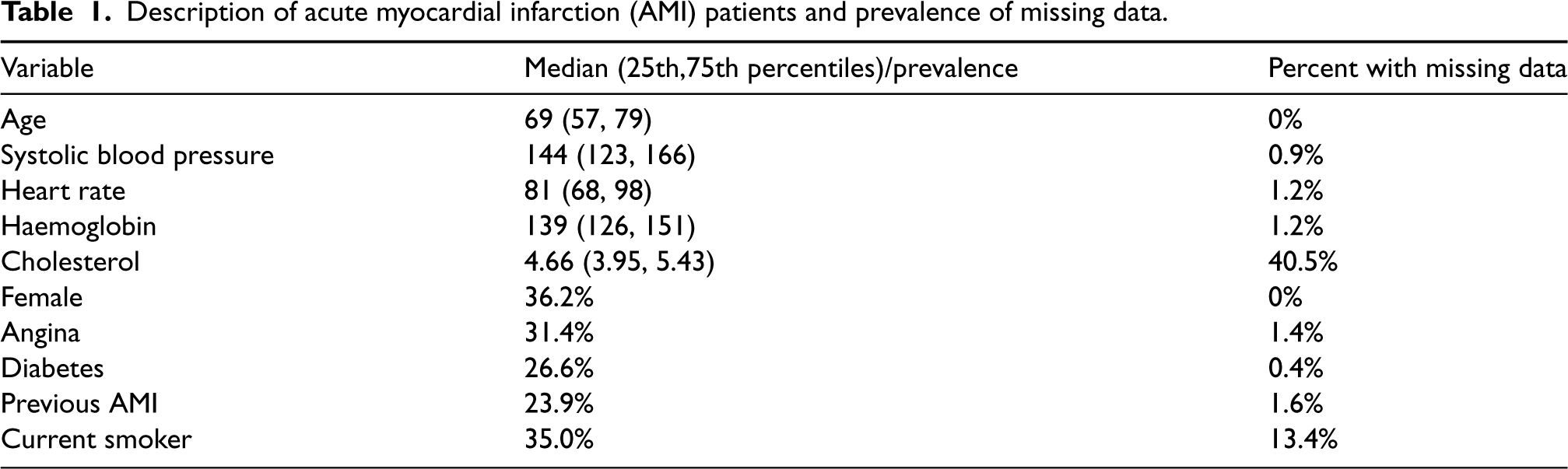
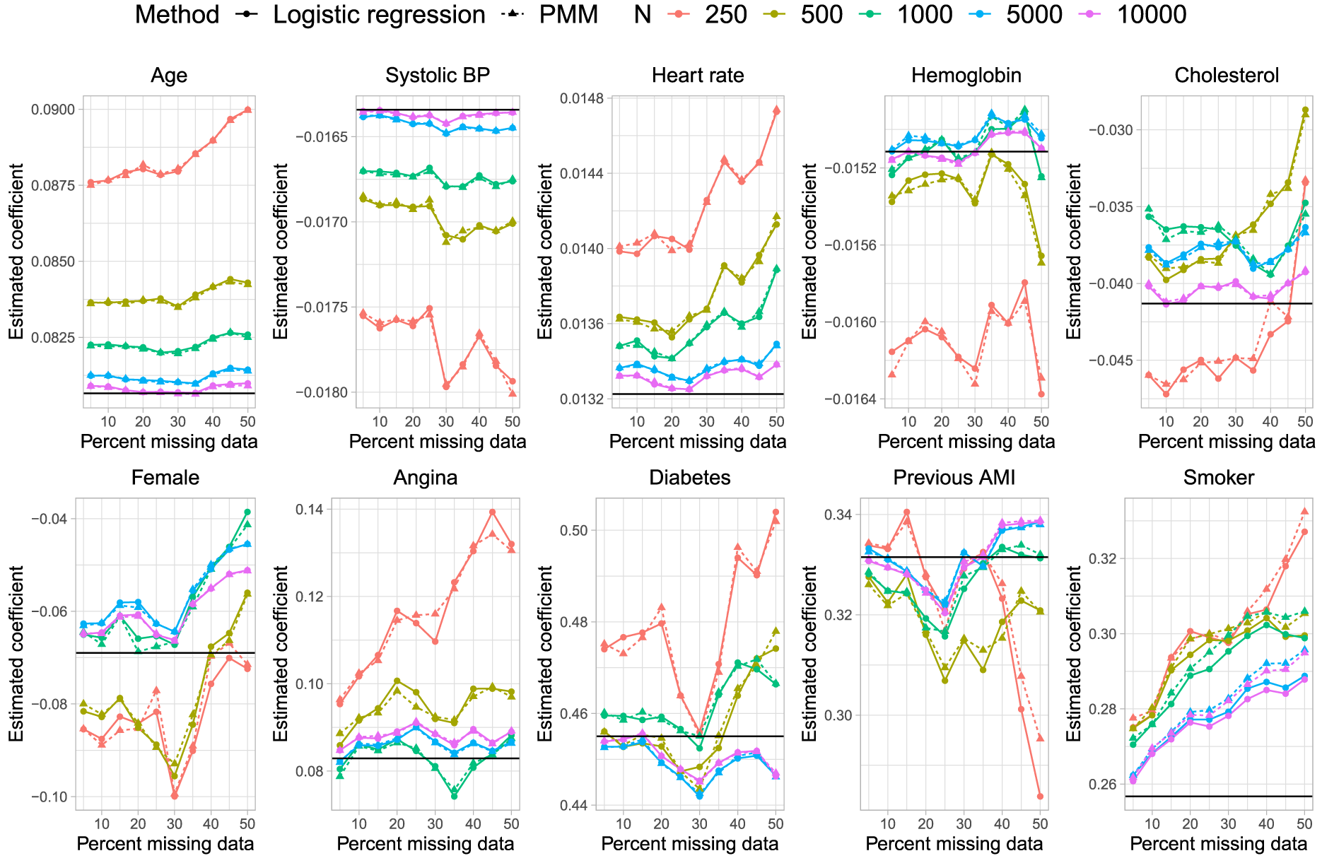
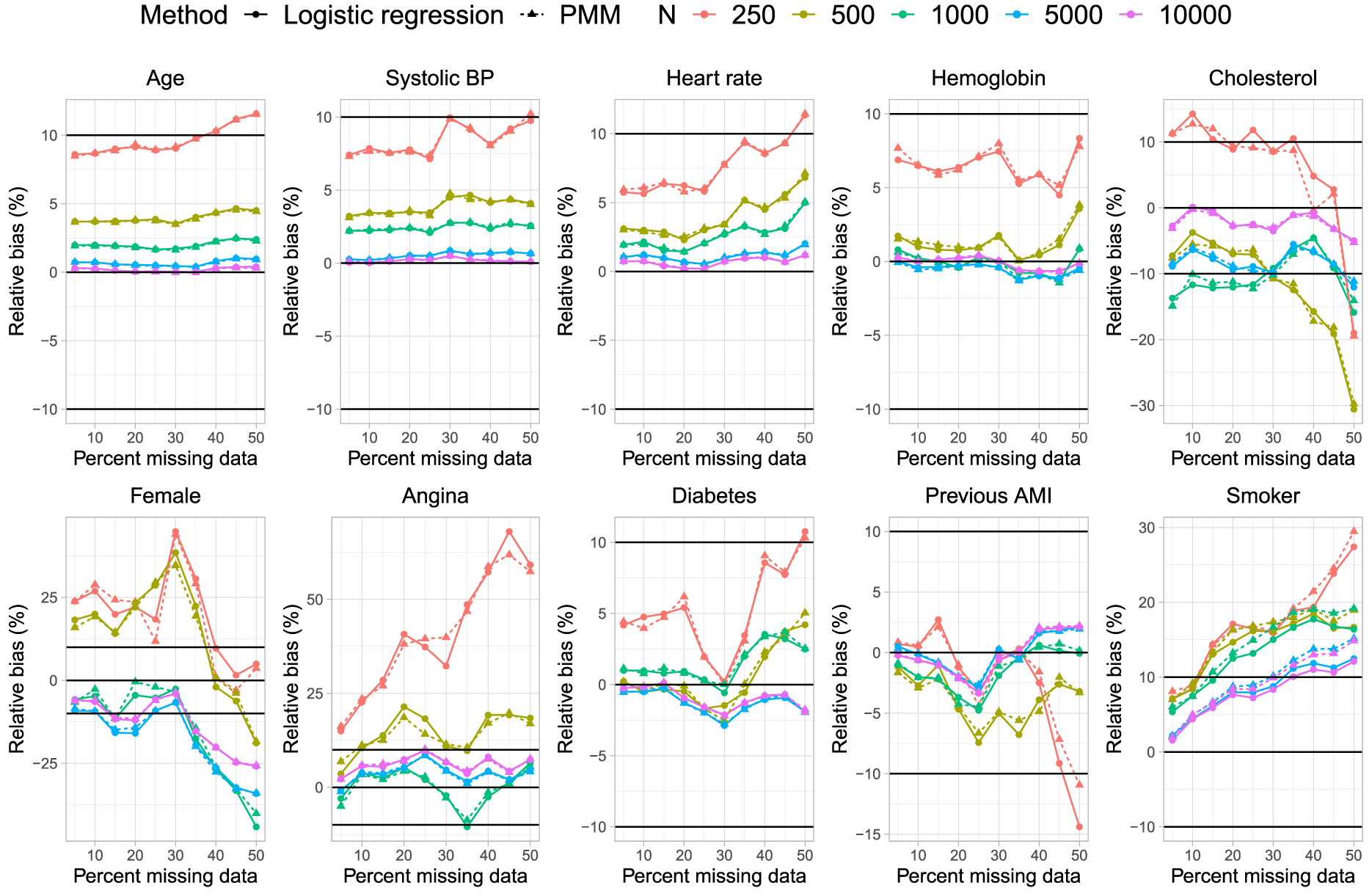
Results are reported in Figure 1 (mean estimated regression coefficient), Figure 2 (relative bias), Figure 3 (standard deviation of estimated regression coefficients across the 1000 simulation replicates), Figure 4 (mean estimated standard error of the estimated regression coefficients across the 1000 simulation replicates), Figure 5 (ratio of estimated to empirical standard error), Figure 6 (MSE), and Figure 7 (coverage of empirical 95% confidence intervals). Each figure consists of 10 panels, one for each of the predictor variables in the analysis model. Within each panel there are 10 lines, one for each combination of sample size (N = 250, 500, 1,000, 5,000, and 10,000) and imputation method for missing binary variables (logistic regression vs. PMM). In each panel, the comparison of greatest interest is between the two lines for the two estimation methods when the sample size was the same. To facilitate this comparison, pairs of lines for the same sample size are depicted using the same colour.
Mean estimated regression coefficient.
Relative bias in estimated regression coefficients (%).
Standard deviation of estimated coefficient across simulation replicates.
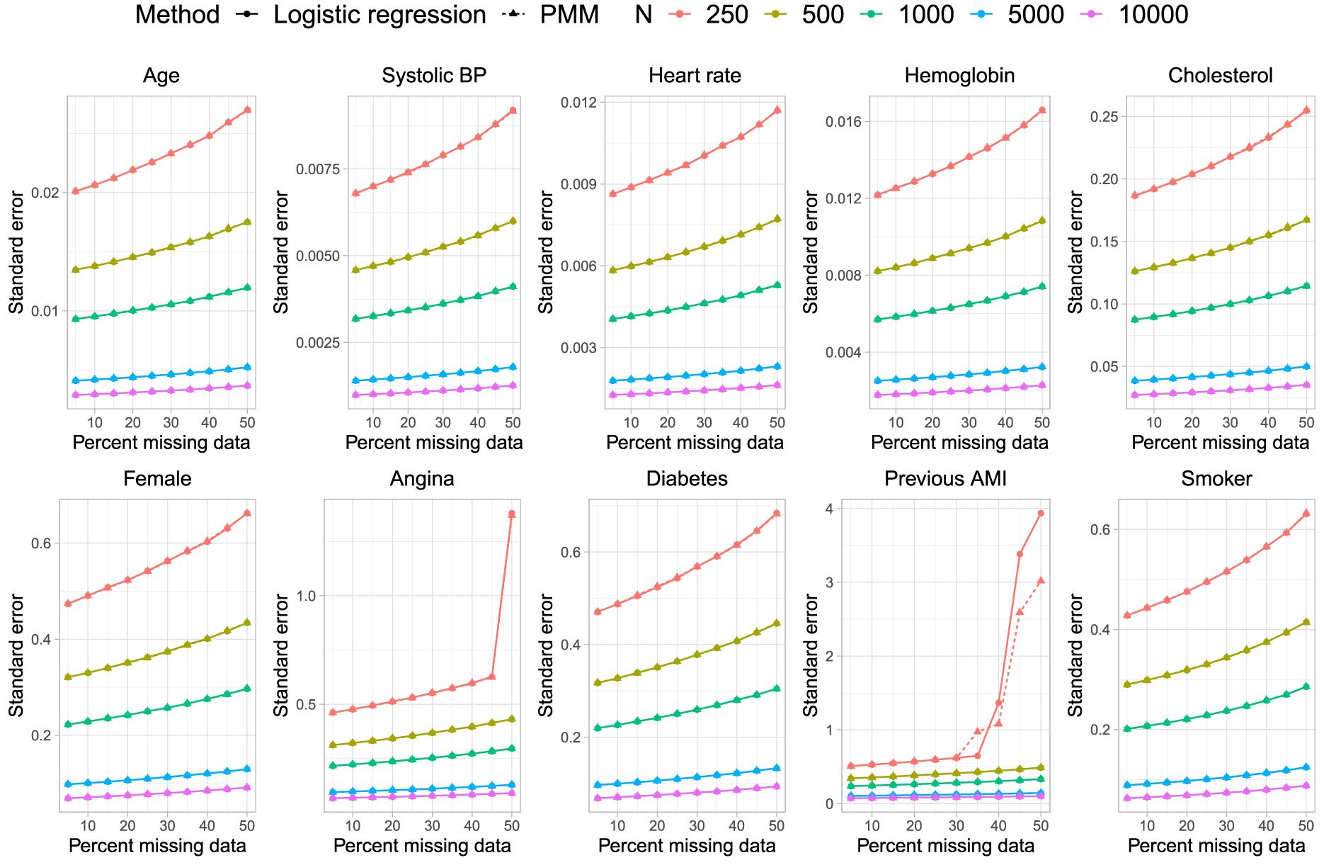
Estimated standard error.
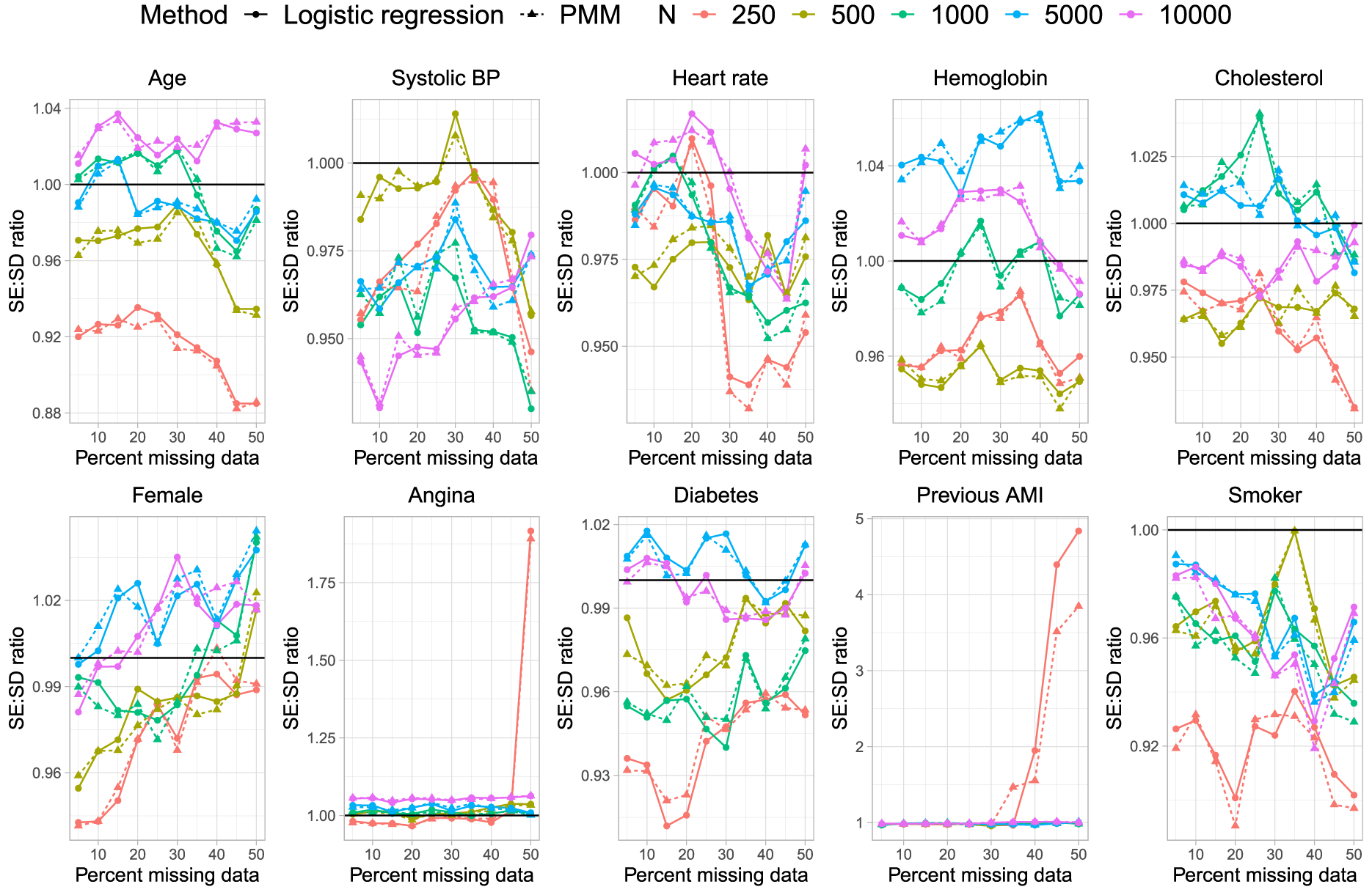
Ratio of estimated to empirical SE.
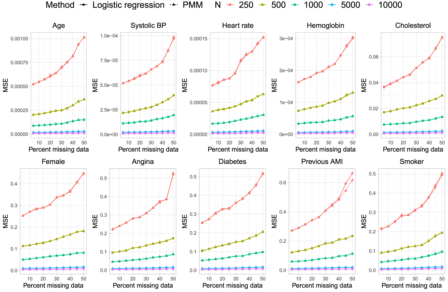
Mean squared error.
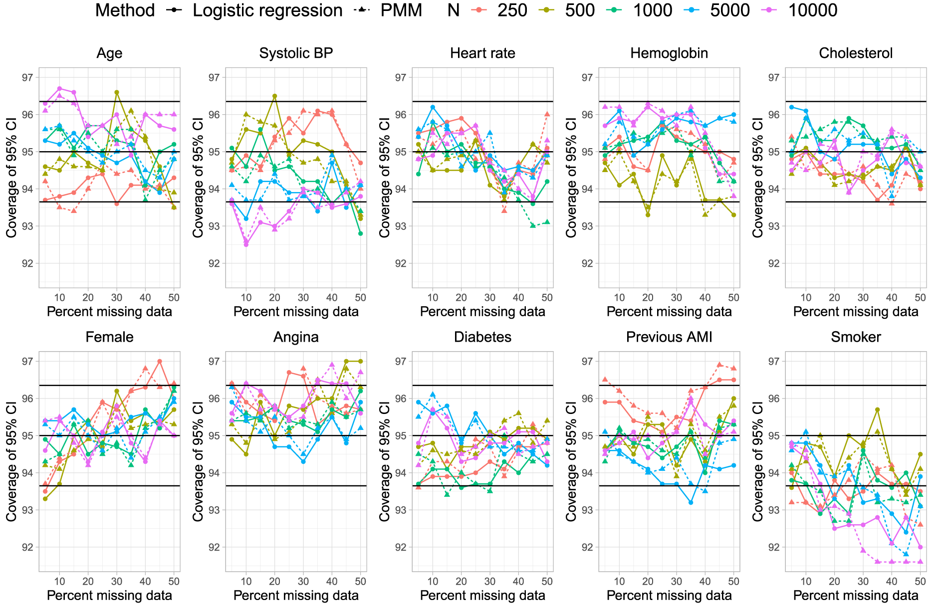
Empirical coverage rates of 95% CIs.
In Figure 1 we have superimposed a horizontal line on each panel denoting the true regression parameter when the analysis model was fit to the super-population with no missing data, while on Figure 2 we have superimposed three horizontal lines denoting relative biases of −10%, 0%, and 10%. Overall, there were no differences in bias in the estimated regression coefficients between the two imputation methods, regardless of sample size. The one exception to this observation was in estimating the regression coefficient for current smokers, the binary variable with the highest prevalence of missing data, when the sample size was 5000 or 10,000 and the prevalence of missing data was at least 40%. In these specific settings, the use of logistic regression for the imputation of missing binary variables resulted in estimates with slightly less bias than did the use of PMM. However, even in these settings, the absolute difference in relative bias was less than 5%. It is possible that setting the donor size to 5 is too low for large sample sizes, resulting in too many duplicates. In general, the observed behaviour is as expected: the bias decreased with increasing sample size and differences in bias between smaller sample sizes were larger than differences in bias between larger sample sizes. The apparent erratic estimates of bias as a function of the percentage of missing data when sample sizes were small to moderate were likely simply a reflection of stochastic variation (recall that, as noted above, the relative difference between the regression coefficients estimated in the super-population and the regression coefficients in the outcomes model used for simulating outcomes in the super-population ranged from −5.5% to 10.8%).The interesting finding is that both PMM and logistic regression exhibit very similar patterns, and thus the use of PMM did not introduce any additional biases beyond what was observed with logistic regression.
In Figure 3, we observe that the standard deviation of the estimated regression coefficients across the 1000 simulation replicates was essentially identical, regardless of whether logistic regression or PMM was used for imputing missing binary variables. Similarly, in Figure 4, we observe that the mean estimated standard errors for the estimated regression coefficients in the analysis model were essentially identical regardless of which method was used for imputing missing binary variables.
In Figure 5 we have superimposed a horizontal line denoting a ratio of 1, indicating that the estimated standard error is accurately estimating the standard deviation of the sampling distribution of the regression coefficient. As with the previous metrics, we did not observe meaningful differences between the two methods for imputing missing binary variables.
As would be anticipated, based on the results for bias and the standard errors of the estimated regression coefficients, the MSE of the estimated coefficients was essentially identical regardless of which method was used for imputing missing binary variables (Figure 6).
On Figure 7 we have superimposed three horizontal lines denoting empirical coverage rates of 93.65%, 95%, and 96.35%. Given our use of 1000 simulation replicates, empirical coverage rates that are less than 93.65% or greater than 96.35% are statistically significantly different from the advertised rate of 95% using a standard normal-theory test (using a type I error rate of 5%). There were no meaningful differences in empirical coverage rates between the two methods for imputing missing binary variables.
We compared the performance of PMM with that of logistic regression for imputing missing binary variables. We evaluated their performance in the context of the analysis model of scientific interest being a logistic regression model. We found that, in general, there were no differences in estimating the analysis model regardless of which method was used for imputing missing binary variables.
The motivation for the study was that imputation of binary variables using PMM is less computationally demanding compared to using logistic regression as the imputation model. This reduced computational demand was observed in our simulations. For instance, in the simulations, for the scenario with sample size of 10,000 and prevalence of missing data equal to 0.50, the use of PMM required 29.2 h using slurm jobs limited to 1 CPU and 4 GB of memory on a grid of compute servers (8 vCPUs – Intel Xeon CPU E5-2643 v3 @ 3.40 GHz, 128GB per node), running RedHat 7, while the use of logistic regression required 87.1 h. Thus, PMM was approximately 3 times more efficient from a computational perspective. This suggests that when evaluating statistical procedures using Monte Carlo simulations, there is a great advantage to using PMM to impute missing binary variables. While our primary motivation was to examine whether PMM could be used to impute missing binary variables when conducting Monte Carlo simulations, we also think that PMM can be used imputing missing variables in empirical analyses.
The current study is subject to certain limitations. First, our study relied on Monte Carlo simulations. Consequently, our findings are dependent on the data-generating process that was used. However, a strength of our simulations was the use of a data-generating process that was based on empirical analyses of patients hospitalized with AMI. Thus, we compared the performance of two methods for imputing missing binary variables in a clinically realistic setting. Many simulations that use a set of independent standard normal distributions for the covariates, result in simulated data that do not reflect any real-world setting. It is possible that PMM may have inferior performance compared to the use of logistic regression in other settings. We suggest that our methods be replicated in other settings to examine the generalizability of our findings. Second, we did not include an examination of the complete case estimator, which is often included in studies examining the performance of MI-based estimators. The rationale for this omission was that we were motivated by examining whether PMM could be used instead of logistic regression for imputing missing binary variables. We were not interested in comparing how each imputation method compared with the use of a complete case analysis.
We hypothesize that one reason that PMM was shown to perform well in our setting was that the prevalence of binary variables ranged from 23.9% to 36.2% (Table 1). The logistic regression model uses the logistic function to transform probabilities into linear predictor. The logistic function is approximately linear when probabilities are not very low or very high. In subjects for whom the probability of the outcome is not extreme, it is likely that the logistic model can be reasonably approximated by a linear model. Since the linear model is only being used to identify a set of subjects from whom one subject is selected at random, the matching process may be relatively robust to minor model mis-specification. We speculate that the relative performance of PMM to that of logistic regression could deteriorate when the prevalence of the binary variable that is subject to missingness is very low or very high.
PMM was proposed by both Rubin 13 and Little. 14 Vink et al. 15 successfully used PMM to impute semi-continuous variables, often with better statistical performance and certainly with faster imputations compared with a dedicated 2-step model. Logistic regression can be affected by problems related to perfect prediction (particularly when one variable perfectly or nearly perfectly predicts the binary outcome), 16 while PMM avoids such problems. Hardt et al. (2013) pushed logistic regression-based imputation methods to their limits and observed that most methods break down relatively quickly (i.e., if the proportion of missing values exceeds 0.4). Problems become worse if the imputation model has binary predictors with low prevalence (e.g., from dummy-coded categorical data). Similarly, van der Palm et al. found that the use of logistic regression to impute binary covariates could fail to identify three-way interactions in the data, resulting in biased parameter estimates. 17 Wu et al. 18 recommended that logistic regression not be used for imputing binary variables as it can result in biased parameter estimates. Audigier et al. 19 found that the use of logistic regression to impute binary variables can result in confidence intervals with sub-optimal coverage rates in datasets with a large number of categories. Van Buuren and Groothuis-Oudshoorn suggested that PMM be used as a faster alternative to logistic regression for imputing binary variables (or to the multinomial logit model for predicting non-binary categorical variables), but provided no evidence on the statistical performance of using PMM for this purpose. 5 We are unaware of previous studies that have compared the performance of PMM with that of logistic regression for imputing missing binary variables. Given the problems with the use of logistic regression highlighted above and that the developer of the MICE algorithm has suggested that PMM be used for imputing binary variables, the current study addresses an important gap in the existing literature on the application of MI methods.
Conclusions
In some settings, PMM can be used to impute missing binary variables when the analysis model of scientific interest is a logistic regression model.
Footnotes
Availability of data
The dataset from this study is held securely in coded form at ICES. While legal data sharing agreements between ICES and data providers (e.g., healthcare organizations and government) prohibit ICES from making the dataset publicly available, access may be granted to those who meet pre-specified criteria for confidential access, available at ![]() (email: das@ices.on.ca).
(email: das@ices.on.ca).
Declaration of conflicting interests
The authors declared no potential conflicts of interest with respect to the research, authorship, and/or publication of this article.
Ethical approval
The use of the data in this project is authorized under section 45 of Ontario's Personal Health Information Protection Act (PHIPA) and does not require review by a Research Ethics Board.
Funding
The authors disclosed receipt of the following financial support for the research, authorship, and/or publication of this article: This work was supported by the Canadian Institutes of Health Research (grant number PJT 166161). ICES is an independent, non-profit research institute funded by an annual grant from the Ontario Ministry of Health (MOH) and the Ministry of Long-Term Care (MLTC). As a prescribed entity under Ontario's privacy legislation, ICES is authorized to collect and use health care data for the purposes of health system analysis, evaluation and decision support. Secure access to these data is governed by policies and procedures that are approved by the Information and Privacy Commissioner of Ontario. The opinions, results and conclusions reported in this paper are those of the authors and are independent from the funding sources. No endorsement by ICES or the Ontario MOH or MLTC is intended or should be inferred. The dataset from this study is held securely in coded form at ICES.