Sage Journals: Discover world-class research

Abstract

Multivariate imputation using chained equations is a popular algorithm for imputing missing data that entails specifying multivariable models through conditional distributions. Two standard imputation methods for imputing missing continuous variables are parametric imputation using a linear model and predictive mean matching. The default methods for imputing missing categorical variables are parametric imputation using multinomial logistic regression and ordinal logistic regression for imputing nominal and ordinal categorical variables, respectively. There is a paucity of research into the relative computational burden and the quality of statistical inferences when using predictive mean matching versus parametric imputation for imputing missing non-binary categorical variables. We used simulations to compare the performance of predictive mean matching with that of multinomial logistic regression and ordinal logistic regression for imputing categorical variables when the analysis model of scientific interest was a logistic or linear regression model. We varied the sample size (N = 500, 1000, 2500, and 5000), the rate of missing data (5%–50% in increments of 5%), and the number of levels of the categorical variable (3, 4, 5, and 6). In general, the performance of predictive mean matching compared very favorably to that of multinomial or ordinal logistic regression for imputing categorical variables when the analysis model was a logistic or linear regression model. This was true across a range of scenarios defined by sample size and the rate of missing data. Furthermore, the use of predictive mean matching was substantially faster, by a factor of 2–6. In conclusion, predictive mean matching can be used to impute categorical variables. The use of predictive mean matching to impute missing non-binary categorical variables substantially reduces computer processing time when conducting multiple imputation.

Keywords

Missing data multiple imputation Monte Carlo simulations

1 Background

Multiple imputation (MI) is a statistical method for addressing missing data.¹ It involves the creation of M (M > 1) complete datasets, in which missing values have been replaced by plausible values generated using an imputation model. A separate statistical analysis is then conducted in each of the M complete datasets, and the results are pooled across the M complete datasets. The foundation of MI is an algorithm for generating plausible values to replace missing observations.

Fully conditional specification (FCS) is an MI algorithm that specifies multivariable models through conditional distributions (e.g. for a continuous variable that is subject to missingness [e.g. weight], the distribution of weight conditional on other variables [e.g. age, sex, education, etc.] is determined using a linear regression model using the other variables as predictors). A popular algorithm for implementing FCS is the MI using chained equations (MICE) algorithm, in which each variable is imputed conditional on all other variables.^2–5 Thus, linear regression can be used for imputing continuous variables (e.g. weight), logistic regression can be used for imputing binary variables (e.g. presence or absence of diabetes), a multinomial logistic regression model can be used for imputing missing nominal (or unordered) categorical variables (e.g. race), and an ordinal logistic regression model can be used for imputing missing ordinal (or ordered) categorical variables (e.g. cancer stage). We refer to this approach as parametric imputation, as the imputed values are generated from a parametric statistical model.

The algorithm for parametric imputation for missing nominal categorical data using a multinomial logistic regression model can be described as follows (see Algorithm 3.3 in the cited reference)²: first, using subjects with complete data, one estimates the regression coefficients for the multinomial logistic regression model that is being used as the imputation model. The parameters of the multinomial logistic regression model and its variance-covariance matrix are estimated using iteratively reweighted least squares (IRLS). Second, one draws a set of regression coefficients for the imputation model from the posterior distribution of regression coefficients using the quantities obtained in the first step. Third, for each subject for whom the categorical variable is missing, one estimates Pr(Z = j), for j = 1, …, K (where Z denotes the K-level categorical variable that is being imputed), using the regression coefficients obtained in the second step and the set of predictor variables in the imputation model, followed by a random draw from the categories based on the subject's K probabilities. Before fitting the model, the data are augmented, as suggested by White et al.,⁶ to avoid problems with perfect separation. A similar approach imputes ordinal variables using ordinal logistic regression under the additional assumption that the categories are ordered.

When variables are continuous, predictive mean matching (PMM) is a fast and robust alternative to parametric imputation using a linear model.² For a subject with missing data on a given variable, PMM identifies those subjects with no missing data on that variable whose linear predictors (computed using the regression coefficients from the fitted imputation model) are close to the linear predictor of the given subject (created using the regression coefficients sampled from the appropriate posterior distribution). Of those subjects who are close, one subject is selected at random, and the observed value of the given variable for that randomly selected subject is used as the imputed value of the variable for the subject with missing data.

It was recently shown that PMM could also be used to impute missing binary variables by treating the binary variable as a continuous variable and that inferences obtained about the coefficients of the analysis model when using PMM were essentially identical to inferences obtained when using a conventional logistic regression model as the imputation model.⁷ Using PMM to impute incomplete binary variables was about three times faster than parametric imputation using a logistic regression model. Computation time is related to the estimation method. PMM fits an imputation model using ordinary least squares regression. The regression coefficients and their variance-covariance matrix can be estimated using closed-form expressions. In contrast, imputation using logistic regression fits the imputation model using IRLS, an iterative procedure. Thus, the estimation of the regression coefficients and the associated variance-covariance matrix takes more processing time for the logistic imputation model than for the linear imputation model. Due to the iterative nature of FCS, the reduction in processing time when using PMM rather than logistic regression can be substantial.

The mice package for the R statistical programming language is one of the most frequently used software packages for implementing MI. The default imputation models for ordinal and nominal categorical variables are ordinal logistic regression and multinomial logistic regression, respectively. While van Buuren and Groothuis-Oudshoorn suggested that PMM could be a faster alternative to multinomial logistic regression for imputing nominal categorical variables, they provided no evidence on the performance of using PMM for this purpose.⁵ Indeed, there is a paucity of information on the relative performance of PMM compared with multinomial logistic regression and ordinal logistic regression for imputing categorical variables.

The mice version 3.16.4 package added new functionality for using PMM to impute ordinal and nominal categorical variables. Before 3.16.4, PMM with categorical data employed the internal integer codes of categorical variables as the dependent variable in the imputation model. With ordinal variables, these levels are monotonically related to the order of the categories, which approaches the numerical case when the inter-category distances can be considered constant. However, for nominal variables, the integer codes are in alphabetic order by default and have no sensible interpretation. The new functionality quantifies the categories by optimizing the canonical correlation between the dummy-coded version of the incomplete variable and the predictors of the imputation model.⁸

The quantification process works as follows. Let $y_{obs}$ be the observed categorical response vector, and $X_{obs}$ its corresponding covariate matrix in the imputation model for $y_{mis}$ . First, we construct the indicator matrix G, an $n_{1} \times K$ binary matrix indicating the category membership of each observation in $y_{obs}$ . Next, we perform canonical correlation analysis (CCA) between G and $X_{obs}$ , yielding the canonical coefficient matrices A and B, which maximize the correlation between linear summaries of G and $X_{obs}$ , respectively. The transformed continuous variable $y_{num}$ is then obtained as $y_{num} = G A_{2}$ , where $A_{2}$ is the second canonical vector. The first canonical correlation equals 1 because it corresponds to the intercept term, and hence contains no useful information. In principle, we could proceed with the higher canonical correlations to provide additional quantified versions of $y_{obs}$ , as suggested by Gifi.⁸ However, for simplicity, we restrict our approach to a single quantification and use $y_{num}$ as the dependent variable in conventional PMM for continuous data. The theoretical basis for CCA is well established. It builds on methods for transforming categorical variables to linearize associations, going back to methods developed by Hotelling⁹ and further developed by Gifi,⁸ by Breiman and Friedman's ACE,¹⁰ and by Harrell's transcan().¹¹ These methods extend classical multivariate techniques, including CCA, to handle categorical variables through optimal scaling or transformation.

The quantification method transforms the relationships in the imputation model into a linear framework, facilitating the association between the incomplete variable and its predictors. Since the transformation is derived from the subset of observed outcomes, it inherently assumes a MAR mechanism. While the imputed values always retain the original category order, the quantification method allows for a different internal ordering within the imputation model. If a strict ordinal structure is required, this flexibility can be constrained using monotone regression. However, enforcing monotonicity may introduce additional noise in the imputations.

After quantification, the imputation model is fitted, and the predicted values from that model are used to measure the similarity of predictive matches. Apart from being faster, the method is expected to be insensitive to the order of categories of nominal variables and to avoid problems related to perfect prediction. However, the relative quality of the inferences about the regression coefficients of the analysis model is not known.

Nominal categorical variables are common when describing individuals’ demographic characteristics, with examples including race (e.g. White, Black, Asian, and Other), marital status (e.g. never married, married, widowed, and divorced), and job category. Nominal categorical variables occur frequently in medical and epidemiological research, with examples including blood type and smoking status (e.g. current smoker vs. recent smoker vs. former smoker vs. never smoker). Similarly, ordinal categorical variables are common (e.g. cancer stage or symptom severity). Given the abundance of nominal and ordinal categorical variables and the high rates of missing data across all research disciplines, it is imperative to determine the optimal method for imputing incomplete categorical data.

Given the importance of nominal and ordinal categorical variables across a wide range of research disciplines, we sought to answer two questions: first, what is the relative difference in computational efficiency between PMM and multinomial and ordinal logistic regression when imputing missing nominal and ordinal categorical variables. Second, to compare the quality of statistical inferences between using PMM and multinomial logistic regression for imputing nominal categorical data, and between using PMM and ordinal logistic regression for imputing ordinal categorical data. As a test case, we considered scenarios in which the analysis model of scientific interest is either a logistic regression model or a linear regression model, and a categorical explanatory or predictor variable is subject to missingness. The article is structured as follows. In Section 2, we provide an empirical case study comparing the performance of PMM with multinomial logistic regression for imputing a nominal categorical variable (smoking history) in a large sample of patients hospitalized with acute myocardial infarction (AMI or heart attack). Section 3 describes the design of a complex series of Monte Carlo simulations to address the study objectives. The design of the Monte Carlo simulations was informed by empirical analyses conducted in patients hospitalized with AMI. In Section 4, we report the results of these simulations. Finally, in Section 5, we summarize our findings and place them in the context of the existing literature.

2 Case study—Individuals hospitalized with AMI

We provide a case study to compare the performance of PMM with that of multinomial logistic regression for imputing a nominal categorical variable when the analysis model of scientific interest is a multivariable logistic regression model. The scientific question is, in patients hospitalized with an AMI, what is the independent association between an individual's smoking history (categorized as current smoker, former smoker, recent smoker, and never smoker) and the risk of death within one year of hospital admission after adjusting for demographic and presentation characteristics, vital signs on presentation, classic cardiac risk factors, comorbid conditions, and laboratory tests.

2.1 Data

We used data on 11,506 patients hospitalized for AMI at 102 hospitals in Ontario, Canada, between 1 April 1999 and 31 March 2001. These data were collected as part of the Enhanced Feedback for Effective Cardiac Treatment study, an initiative designed to improve the quality of cardiac care in Ontario.¹² Data were collected on demographic characteristics (age and sex); presentation characteristics (cardiogenic shock and acute congestive heart failure/pulmonary edema); vital signs on presentation (systolic blood pressure, diastolic blood pressure, heart rate, and respiratory rate); classic cardiac risk factors (diabetes, hypertension, smoking history, dyslipidemia, and family history of coronary artery disease); comorbid conditions (cerebrovascular disease [i.e. stroke], angina, cancer, dementia, peptic ulcer disease, previous AMI, asthma, depression, peripheral vascular disease, previous revascularization, congestive heart failure, hyperthyroidism, and aortic stenosis); and laboratory tests (hemoglobin, white blood count, sodium, potassium, glucose, urea, and creatinine). Age, the four vital signs on presentation, and the seven laboratory tests were continuous. Smoking history was a four-level nominal categorical variable: never smoker versus current smoker versus recent smoker, versus former smoker. The remaining variables were binary variables. In the current case study, the outcome was a binary variable denoting death within one year of hospital admission. Two thousand three hundred and eight (20.0%) individuals died within one year of hospital admission.

Forty-five percent of individuals had missing data on at least one of the variables listed above. Except for age and sex (which were available from provincial registries), all variables were subject to missingness. Smoking history was missing for 14.6% of subjects. Of those with an observed smoking history variable, 3320 (33.8%) were never smokers, 3729 (38.0%) were current smokers, 2579 (26.3%) were former smokers, and 194 (2.0%) were recent smokers.

2.2 Statistical analyses

The analysis model of scientific interest was a logistic regression model in which the binary variable denoting death within one year of hospital admission was regressed on all the other variables listed above.

We used MI to create 45 complete datasets (the number of complete datasets was set equal to the percentage of subjects with any missing data³). PMM was used to impute the missing continuous and binary variables, while multinomial logistic regression was used to impute missing values of smoking history, which was a nominal four-level categorical variable. For each variable that was subject to missingness, the imputation model included all the other variables listed above, including the binary outcome for the scientific model of interest.³

In each of the 45 complete datasets, we regressed the binary outcome variable denoting death within one year of hospital admission on all the other variables listed above using a logistic regression model. For each variable, the estimated regression coefficients and associated standard errors were pooled across the 45 complete datasets using Rubin's rules.

We then repeated the entire process using PMM to impute all variables that were subject to missingness, including the four-level nominal categorical variable denoting smoking history.

R code for the analyses conducted in this case study is available in the first author's GitHub repository [https://github.com/peter-austin/2025-SMMR-PMM_imputing_categorical_variables].

2.3 Results

Creating the 45 complete datasets required 52.0 min when using multinomial logistic regression to impute smoking history and 22.9 min when using PMM to impute smoking history (using slurm jobs limited to 1 CPU and 4 GB of memory on a grid of compute servers [8 vCPUs – Intel Xeon CPU E5-2643 v3 at 3.40 GHz, 128GB per node], running RedHat 7). Thus, the use of multinomial logistic regression required ∼2.3 times more time than did PMM.

After using multinomial logistic regression to impute smoking history, the pooled prevalence of the four levels of smoking history across the 45 complete datasets were 35.2% (never smoker), 36.3% (current smoker), 26.6% (former smoker), and 1.9% (recent smoker). Identical estimates of the pooled prevalences were obtained when using PMM to impute smoking history. Thus, using PMM instead of multinomial regression did not change the estimated prevalence of each of the four categories of smoking history.

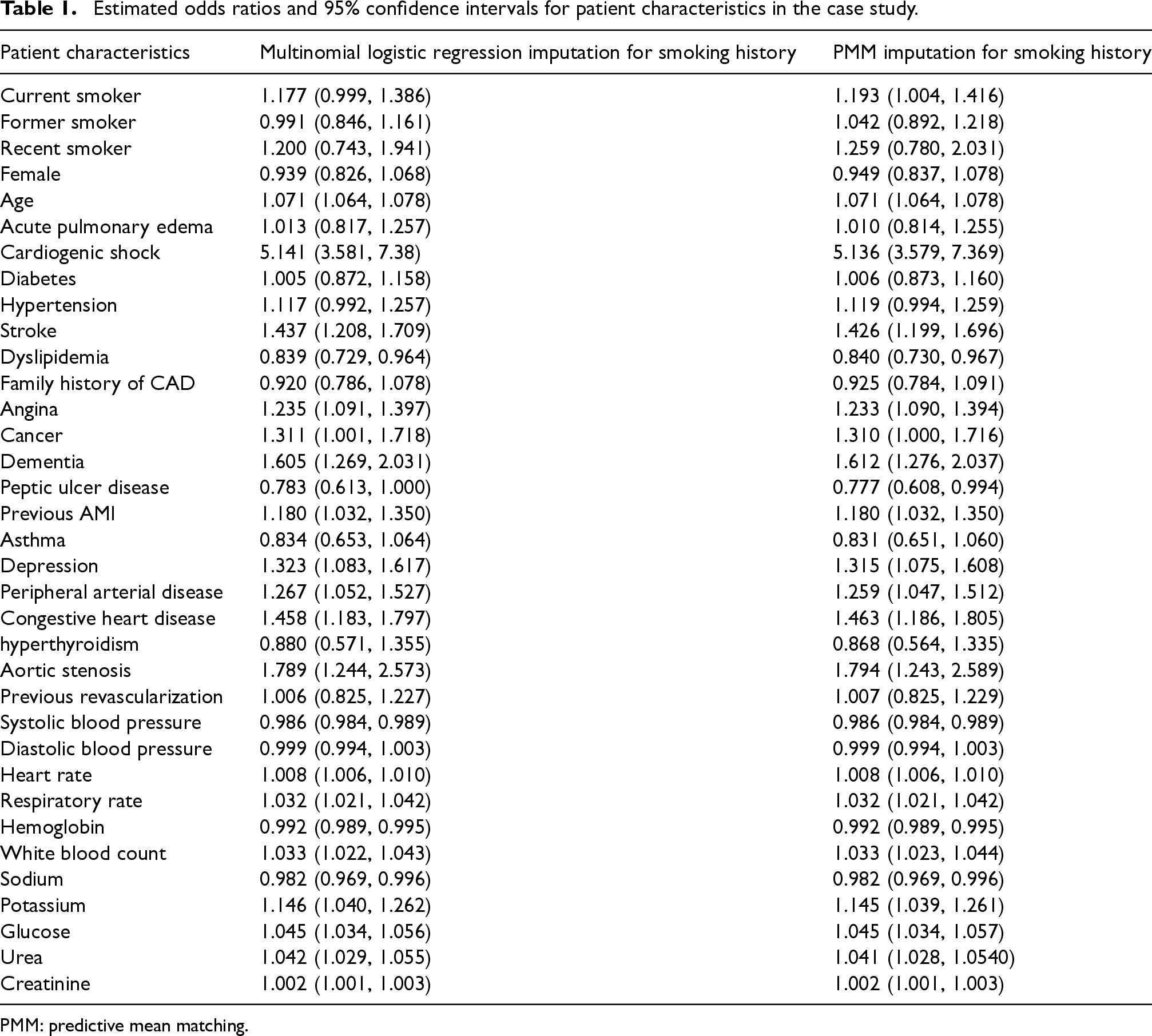
The estimated odds ratios (obtained by exponentiating the pooled estimates of the regression coefficients) and their associated 95% confidence intervals for all the variables in the logistic regression model are reported in Table 1. In our discussion of the results, we focus on the estimated odds ratios for smoking history. When using multinomial logistic regression to impute smoking history, the estimated odds ratio for being a current smoker at the time of hospital admission was 1.177 (95% CI: 0.999–1.386). Thus, being a current smoker at the time of hospital admission was associated with a 17.7% increase in the odds of death within one year compared with those who had never smoked. The estimated odds ratio for being a former smoker was 0.991 (95% CI: 0.846–1.161). Thus, being a former smoker was associated with a 0.9% decrease in the odds of death within one year compared with those who had never smoked. The estimated odds ratio for being a recent smoker was 1.200 (95% CI: 0.743–1.941). Thus, being a recent smoker was associated with a 20.0% increase in the odds of death within one year compared to those who had never smoked. All three 95% confidence intervals contained the null value; thus, none of these estimated relative changes in the odds of death were statistically significantly different from the null. When using PMM to impute smoking history, the estimated odds ratio for being a current smoker at the time of hospital admission was 1.193 (95% CI: 1.004–1.416). Thus, being a current smoker at the time of hospital admission was associated with a 19.3% increase in the odds of death within one year compared with those who had never smoked. The estimated odds ratio for being a former smoker was 1.042 (95% CI: 0.892–1.218). Thus, being a former smoker was associated with a 4.2% increase in the odds of death within one year compared with those who had never smoked. The estimated odds ratio for being a recent smoker was 1.259 (95% CI: 0.780–2.031). Thus, being a recent smoker was associated with a 25.9% increase in the odds of death within one year compared to those who had never smoked. The 95% confidence intervals for two of the levels of smoking history included the null value. While the estimated odds ratios were not identical between the two imputation approaches, the estimated odds ratios and their associated 95% confidence intervals were qualitatively similar between the two imputation approaches.

Table 1.
Estimated odds ratios and 95% confidence intervals for patient characteristics in the case study.

Patient characteristics Multinomial logistic regression imputation for smoking history PMM imputation for smoking history

Current smoker 1.177 (0.999, 1.386) 1.193 (1.004, 1.416)

Former smoker 0.991 (0.846, 1.161) 1.042 (0.892, 1.218)

Recent smoker 1.200 (0.743, 1.941) 1.259 (0.780, 2.031)

Female 0.939 (0.826, 1.068) 0.949 (0.837, 1.078)

Age 1.071 (1.064, 1.078) 1.071 (1.064, 1.078)

Acute pulmonary edema 1.013 (0.817, 1.257) 1.010 (0.814, 1.255)

Cardiogenic shock 5.141 (3.581, 7.38) 5.136 (3.579, 7.369)

Diabetes 1.005 (0.872, 1.158) 1.006 (0.873, 1.160)

Hypertension 1.117 (0.992, 1.257) 1.119 (0.994, 1.259)

Stroke 1.437 (1.208, 1.709) 1.426 (1.199, 1.696)

Dyslipidemia 0.839 (0.729, 0.964) 0.840 (0.730, 0.967)

Family history of CAD 0.920 (0.786, 1.078) 0.925 (0.784, 1.091)

Angina 1.235 (1.091, 1.397) 1.233 (1.090, 1.394)

Cancer 1.311 (1.001, 1.718) 1.310 (1.000, 1.716)

Dementia 1.605 (1.269, 2.031) 1.612 (1.276, 2.037)

Peptic ulcer disease 0.783 (0.613, 1.000) 0.777 (0.608, 0.994)

Previous AMI 1.180 (1.032, 1.350) 1.180 (1.032, 1.350)

Asthma 0.834 (0.653, 1.064) 0.831 (0.651, 1.060)

Depression 1.323 (1.083, 1.617) 1.315 (1.075, 1.608)

Peripheral arterial disease 1.267 (1.052, 1.527) 1.259 (1.047, 1.512)

Congestive heart disease 1.458 (1.183, 1.797) 1.463 (1.186, 1.805)

hyperthyroidism 0.880 (0.571, 1.355) 0.868 (0.564, 1.335)

Aortic stenosis 1.789 (1.244, 2.573) 1.794 (1.243, 2.589)

Previous revascularization 1.006 (0.825, 1.227) 1.007 (0.825, 1.229)

Systolic blood pressure 0.986 (0.984, 0.989) 0.986 (0.984, 0.989)

Diastolic blood pressure 0.999 (0.994, 1.003) 0.999 (0.994, 1.003)

Heart rate 1.008 (1.006, 1.010) 1.008 (1.006, 1.010)

Respiratory rate 1.032 (1.021, 1.042) 1.032 (1.021, 1.042)

Hemoglobin 0.992 (0.989, 0.995) 0.992 (0.989, 0.995)

White blood count 1.033 (1.022, 1.043) 1.033 (1.023, 1.044)

Sodium 0.982 (0.969, 0.996) 0.982 (0.969, 0.996)

Potassium 1.146 (1.040, 1.262) 1.145 (1.039, 1.261)

Glucose 1.045 (1.034, 1.056) 1.045 (1.034, 1.057)

Urea 1.042 (1.029, 1.055) 1.041 (1.028, 1.0540)

Creatinine 1.002 (1.001, 1.003) 1.002 (1.001, 1.003)

Patient characteristics	Multinomial logistic regression imputation for smoking history	PMM imputation for smoking history
Current smoker	1.177 (0.999, 1.386)	1.193 (1.004, 1.416)
Former smoker	0.991 (0.846, 1.161)	1.042 (0.892, 1.218)
Recent smoker	1.200 (0.743, 1.941)	1.259 (0.780, 2.031)
Female	0.939 (0.826, 1.068)	0.949 (0.837, 1.078)
Age	1.071 (1.064, 1.078)	1.071 (1.064, 1.078)
Acute pulmonary edema	1.013 (0.817, 1.257)	1.010 (0.814, 1.255)
Cardiogenic shock	5.141 (3.581, 7.38)	5.136 (3.579, 7.369)
Diabetes	1.005 (0.872, 1.158)	1.006 (0.873, 1.160)
Hypertension	1.117 (0.992, 1.257)	1.119 (0.994, 1.259)
Stroke	1.437 (1.208, 1.709)	1.426 (1.199, 1.696)
Dyslipidemia	0.839 (0.729, 0.964)	0.840 (0.730, 0.967)
Family history of CAD	0.920 (0.786, 1.078)	0.925 (0.784, 1.091)
Angina	1.235 (1.091, 1.397)	1.233 (1.090, 1.394)
Cancer	1.311 (1.001, 1.718)	1.310 (1.000, 1.716)
Dementia	1.605 (1.269, 2.031)	1.612 (1.276, 2.037)
Peptic ulcer disease	0.783 (0.613, 1.000)	0.777 (0.608, 0.994)
Previous AMI	1.180 (1.032, 1.350)	1.180 (1.032, 1.350)
Asthma	0.834 (0.653, 1.064)	0.831 (0.651, 1.060)
Depression	1.323 (1.083, 1.617)	1.315 (1.075, 1.608)
Peripheral arterial disease	1.267 (1.052, 1.527)	1.259 (1.047, 1.512)
Congestive heart disease	1.458 (1.183, 1.797)	1.463 (1.186, 1.805)
hyperthyroidism	0.880 (0.571, 1.355)	0.868 (0.564, 1.335)
Aortic stenosis	1.789 (1.244, 2.573)	1.794 (1.243, 2.589)
Previous revascularization	1.006 (0.825, 1.227)	1.007 (0.825, 1.229)
Systolic blood pressure	0.986 (0.984, 0.989)	0.986 (0.984, 0.989)
Diastolic blood pressure	0.999 (0.994, 1.003)	0.999 (0.994, 1.003)
Heart rate	1.008 (1.006, 1.010)	1.008 (1.006, 1.010)
Respiratory rate	1.032 (1.021, 1.042)	1.032 (1.021, 1.042)
Hemoglobin	0.992 (0.989, 0.995)	0.992 (0.989, 0.995)
White blood count	1.033 (1.022, 1.043)	1.033 (1.023, 1.044)
Sodium	0.982 (0.969, 0.996)	0.982 (0.969, 0.996)
Potassium	1.146 (1.040, 1.262)	1.145 (1.039, 1.261)
Glucose	1.045 (1.034, 1.056)	1.045 (1.034, 1.057)
Urea	1.042 (1.029, 1.055)	1.041 (1.028, 1.0540)
Creatinine	1.002 (1.001, 1.003)	1.002 (1.001, 1.003)

PMM: predictive mean matching.

In summary, using PMM to impute missing categorical variables required less than half the time required by multinomial logistic regression. Furthermore, inferences about the association between smoking history and the risk of one-year death were qualitatively similar across the two imputation approaches.

3 Monte Carlo simulations—Methods

We conducted a series of complex Monte Carlo simulations to compare the performance between PMM and multinomial logistic regression for imputing nominal categorical data, and between PMM and ordinal logistic regression for imputing ordinal categorical data. We evaluated the performance of each method in settings in which the analysis model of scientific interest was either a multivariable logistic regression model or a multivariable linear regression model. The design of the Monte Carlo simulations was informed by empirical analyses conducted on the data on patients hospitalized for AMI described in Section 2.1. Thus, the simulated data arereflective of the complexities of medical data observed in clinical research.

3.1 Factors in the Monte Carlo simulations

We allowed three factors to vary in our simulations: N_sample (the size of the random sample drawn from the super-population), p_missing (the rate of missing data), and K (the number of levels of the categorical variable that was subject to missingness). The first took four values: 500, 1000, 2500, and 5000. The second took 10 values: from 5% to 50% in increments of 5%. The third took four levels: from 3 to 6 in increments of one. We used a full factorial design and thus considered 160 different scenarios. In each scenario, we simulated a super-population of size 1,000,000 from which a random sample of size N_sample was sampled in each of the 1000 iterations of the simulations.

3.2 Empirical analyses in the case study to obtain parameters for the data-generating process

3.2.1 Analysis model is a multivariable logistic regression model

We made the decision to simulate nine baseline variables in addition to the K-level categorical variable of interest. This number of baseline covariates would reflect clinically realistic settings, but not be so large as to make the simulations overly computationally burdensome. Using the 45 complete datasets created above, when multinomial logistic regression was used to impute smoking history, we used logistic regression to regress the binary variable denoting death within one year on the variables listed above, with the exception that smoking history was excluded from the set of predictor variables. We selected nine of the variables that had amongst the strongest relationship with one-year mortality: age, systolic blood pressure, heart rate, respiratory rate, glucose, white blood count, urea, creatinine, and hemoglobin. We will simulate nine variables whose multivariate distribution will be similar to that observed for these nine variables in the case study data.

We fit a reduced logistic regression model in each of the 45 complete datasets in which one-year mortality was regressed on these nine predictor variables. For each individual, we determined the linear predictor based on these nine predictor variables. In each complete dataset, we determined the polyserial correlation between the linear predictor and the nominal categorical variable denoting smoking history. We used Rubin's rules to pool the estimated polyserial correlation coefficient across the 45 complete datasets. The estimated polyserial correlation was equal to −0.097. We also used Rubin's rules to pool the intercept and the nine estimated regression coefficients across the 45 complete datasets. Let $β_{9}$ denote the vector of pooled regression coefficients for these nine variables. In the empirical analyses $β_{9} = (- 6.247, 0.073, - 0.016, 0.052, 0.008, 0.036, 0.049, 0.037, 0.003, - 0.010)$ , where the first component is the intercept, and the other nine components are the regression coefficients for the nine baseline variables.

We estimated the mean of each of the nine variables in each of the 45 complete datasets and pooled the resultant means across the 45 complete datasets using Rubin's rules. Similarly, we computed the variance-covariance matrix of the nine variables in each of the 45 complete datasets and pooled the 45 variance-covariance matrices using Rubin's rules. Let $μ_{9}$ and $Σ_{9 \times 9}$ denote the pooled vector of nine means and the pooled 9 × 9 variance-covariance matrix, respectively. The vector of means and the variance-covariance matrix will be used to generate nine variables whose distribution is similar to that of these nine baseline covariates.

In each of the 45 complete datasets, we fit a logistic regression model in which the binary variable denoting death within one year was regressed on the nine variables and the four-level variable denoting smoking history. The estimated regression coefficients were pooled across the 45 complete datasets using Rubin's rules. Let $β_{outcome}$ denote the resultant vector of pooled regression coefficients (including an intercept). Note that in the empirical analyses, this could only be done for a four-level categorical variable (never smoker vs. former smoker vs. recent smoker vs. current smoker). In the empirical analyses, we had that $β_{outcome} = (- 6.437, 0.075, - 0.016, 0.052, 0.008, 0.035, 0.049, 0.036, 0.003, - 0.010, 0.160, 0.003, 0.171)$ , where the first component is the intercept, the next nine components are the regression coefficients for the nine baseline variables, and the last three components are the regression coefficients for being a current smoker, a former smoker, and a recent smoker.

Finally, in each of the 45 complete datasets, we fit a logistic regression model in which a binary variable denoting whether smoking history had been missing for that individual (prior to imputation) was regressed on the nine continuous variables and the binary outcome of the scientific model (one-year mortality). The estimated regression coefficients were pooled across the 45 complete datasets using Rubin's Rules. Let $β_{missing}$ denote the resultant vector of pooled regression coefficients (including an intercept). In the empirical analyses, $β_{missing} = (- 4.311, 0.040, - 0.002, 0.029, 0.001, 0.000, 0.014, 0.002, 0.001, - 0.005, 0.264)$ , where the first component is the intercept, the middle nine components are the regression coefficients for the nine baseline variables, and the last component is the regression coefficient for the binary outcome denoting death within one year. These regression coefficients will be used to induce missing data in the Monte Carlo simulations.

3.2.2 Analysis model is a multivariable linear regression model

We modified the empirical analyses described in Section 3.2.1 to estimate parameters for a data-generating process for simulations in which the analysis model of scientific interest was a multivariable linear regression model. We replaced the binary outcome (death within one year) for the analysis model with a continuous outcome: systolic blood pressure at hospital discharge. For these empirical analyses, we restricted the analytic sample to those 10,368 patients who were discharged alive from the hospital (as only these patients will have a discharge systolic blood pressure). For consistency with the previous empirical analyses, we used the same 10 predictor variables as in Section 3.2.1.

We created 45 complete datasets using multinomial logistic regression to impute smoking history. We fit a linear regression model in each of the 45 complete datasets in which discharge systolic blood pressure was regressed on these nine predictor variables. For each individual, we determined the linear predictor based on these nine predictor variables. In each complete dataset, we determined the polyserial correlation between the linear predictor and the nominal categorical variable denoting smoking history. We used Rubin's rules to pool the estimated polyserial correlation coefficient across the 45 complete datasets. The estimated polyserial correlation was equal to −0.080. We also used Rubin's rules to pool the intercept and the nine estimated regression coefficients across the 45 complete datasets. Let $β_{9}$ denote the vector of pooled regression coefficients for these nine variables. In the empirical analyses $β_{9} = (82.559, 0.213, 0.172, 0.100, 0.029, - 0.109, 0.096, - 0.045, 0.010, - 0.036)$ , where the first component is the intercept, and the other nine components are the regression coefficients for the nine baseline variables. The pooled estimate of the standard deviation of the distribution of the residual or error terms was equal to 18.428, while the pooled estimate of R² across the 45 complete datasets was 18.4%.

In each of the 45 complete datasets, we fit a linear regression model in which discharge systolic blood pressure was regressed on the nine variables and the four-level nominal variable denoting smoking history. The estimated regression coefficients were pooled across the 45 complete datasets using Rubin's Rules. Let $β_{outcome}$ denote the resultant vector of pooled regression coefficients (including an intercept). Note that in the empirical analyses, this could only be done for a four-level categorical variable (never smoker vs. former smoker vs. recent smoker vs. current smoker). In the empirical analyses, we had that $β_{outcome} = (84.036, 0.199, 0.171, 0.094, 0.030, - 0.100, 0.092, - 0.040, 0.010, - 0.034, - 1.322, - 0.909, - 3.249)$ , where the first component is the intercept, the next nine components are the regression coefficients for the nine baseline variables, and the last three components are the regression coefficients for being a current smoker, a former smoker, and a recent smoker.

Finally, as in Section 3.2.1, we estimated the regression coefficients for the missing data model for smoking history. The pooled estimate of the regression coefficients was $β_{missing} = (- 4.581, 0.042, - 0.002, 0.030, 0, - 0.002, 0.018, 0.005, 0.001, - 0.006, 0.001)$ , where the first component is the intercept, the middle nine components are the regression coefficients for the nine baseline variables, and the last component is the regression coefficient for the continuous variable denoting discharge systolic blood pressure. These regression coefficients will be used to induce missing data in the Monte Carlo simulations.

3.3 Monte Carlo simulations: Simulating a super-population

3.3.1 Simulations with a binary outcome for the analysis model

We constructed a vector of 10 means, $μ_{10}$ , where the first nine means were those in $μ_{9}$ (described above), while the last mean was set to zero (i.e. the mean of the tenth variable will be zero; this variable will be subsequently categorized, so the mean of the continuous variable is unimportant). We then constructed a 10 × 10 variance-covariance $Σ_{10 \times 10}$ matrix that incorporated the 9 × 9 variance covariance matrix $Σ_{9 \times 9}$ estimated above for the nine variables listed above. The top left corner comprising the first nine rows and first nine columns of $Σ_{10 \times 10}$ was equal to $Σ_{9 \times 9}$ . The (10, 10) element (i.e. the last element on the diagonal in the 10th row and 10th column) was set equal to 1. The remaining elements in the 10th row and the 10th column were set equal to $τ$ (to be determined in the following paragraph).

For a large super-population consisting of 1,000,000 individuals, we generated 10 continuous variables from a multivariate normal distribution with mean $μ_{10}$ and variance-covariance matrix $Σ_{10 \times 10}$ . Let $X_{1}$ through $X_{9}$ denote the first nine variables. Using the first nine variables, we computed a linear predictor using the vector of regression coefficients $β_{9}$ that was computed above (see above for description of $β_{9}$ ). We then categorized the 10th variable into a K-level categorical variable by using the appropriate quantiles of a standard normal distribution (since the 10th variable was generated to have mean zero and unit variance). Let Z denote the resultant K-level categorical variable. The categorical variable was simulated so that an approximately equal number of individuals were at each of the K levels (Pr(Z = 1) = Pr(Z = 2) = ⋯ = Pr(Z = K)). We computed the polyserial correlation between the linear predictor and the K-level categorical variable. We use a bisection approach to determine the value of $τ$ that resulted in the polyserial correlation being equal to that computed in the empirical analyses above (−0.097).

For the settings in which Z was nominal, we then randomly permuted the labels for this variable so that any implicit ordering in the variable due to the use of the normal distribution was removed (e.g. a random permutation was used so that the labels were changed as follows: 1 → 4; 2 → 5; 3 → 3, 4 → 2; 5 → 1).

We then generated a binary outcome Y for each subject in the super-population. To do so, we applied an outcomes model to each individual in the super-population and computed the probability of the occurrence of the binary outcome. We then simulated a binary outcome from a Bernoulli distribution with this subject-specific parameter. We used the following outcomes logistic models, each of which is specific to a given value of K:

\begin{aligned} (K = 3) logit(Pr(Y = 1)) & = X_{9} β_{outcome,9} + log(1 .25) Z_{2} + log(1 .5) Z_{3} \end{aligned}

\begin{aligned} (K = 4) logit (Pr (Y = 1)) & = X_{9} β_{outcome,9} + \log (1.25) Z_{2} + \log (1.5) Z_{3} + \log (2) Z_{4} \end{aligned}

\begin{aligned} (K = 5) logit (Pr (Y = 1)) & = X_{9} β_{outcome,9} + \log (1.1) Z_{2} + \log (1.25) Z_{3} \\ + \log (1.5) Z_{4} + \log (2) Z_{5} \end{aligned}

\begin{aligned} (K = 6) logit (Pr (Y = 1)) & = X_{9} β_{outcome,9} + \log (1.1) Z_{2} + \log (1.25) Z_{3} \\ + \log (1.5) Z_{4} + \log (1.75) Z_{5} + \log (2) Z_{6} \end{aligned}

where

X_{9}

denotes a vector consisting of an intercept (1) and the first nine variables (X₁–X₉),

β_{outcome, 9}

refers to the intercept and regression coefficients for X₁–X₉ from the outcome model estimated above, Z_j refers to the dummy or binary indicator variable used to represent the jth level of Z, for j = 2, …, K. Thus, the first level of Z (Z = 1) is used as the reference level. Note that the regression coefficients for X₁–X₉ were equal to those estimated in the empirical analyses described above. Since the empirical analyses only used a four-level categorical variable, we chose regression coefficients for the K–1 non-reference levels, rather than allowing them to be dictated by empirical analyses. Apart from this one modification, the data-generating process that we have described results in simulated data reflective of those observed in the empirical data. Thus, our data-generating process reflects both a clinically realistic scenario and the complexity that is often observed in clinical data.

We then fit the outcomes model in the simulated super-population by regressing the simulated binary outcome on the 10 simulated explanatory variables. The estimated regression coefficients will be considered the “true” values of the regression coefficients to which the coefficients estimated below will be compared.

We then induced missing data in the simulated super-population. We assumed that there was only one missing data pattern: Z, the K-level categorical variable, was subject to missingness, while nine continuous variables (X₁ through X₉) and Y (the binary outcome variable) were not subject to missingness. We set the data to missing such that the prevalence of missing data in the super-population was equal to the desired prevalence $(p_{missing})$ . We used a missing at random (MAR) missing data mechanism in which the likelihood of Z being missing was related only to X₁ through X₉ and Y (i.e. missingness in Z was not related to Z).^1,2 In the super-population, we computed the probability of Z (the K-level categorical variable) being missing by using the regression coefficient $β_{missing}$ estimated in the empirical analyses described above. For each individual, we computed the log-odds of Z being missing using a linear predictor computed using $β_{missing}$ and X₁ through X₉ and Y. We used a bisection approach to modify the intercept of the missing data model so that the rate of missing data in the super-population was equal to the desired quantity.

The above data-generating process was for simulating data such that Z was a nominal K-level categorical variable. We used a similar data-generating process for simulating data such that Z was an ordinal K-level categorical variable. Only two modifications were made: (i) we generated data such that Spearman's rank correlation (rather than using the polyserial correlation) between the linear predictor comprised of the first nine continuous variables and the K-level ordinal categorical variable was equal to −0.097; (ii) we did not randomly permute the labels of the K-level categorical variable, but retained the ordering implicit in the categorization of the underlying normal distribution.

3.3.2 Simulations with a continuous outcome for the analysis model

These simulations were similar to those described above, with the following modifications. Instead of using a logistic regression model to simulate binary outcomes, we used a linear model to simulate continuous outcomes. We used the following outcomes linear regression models, each of which is specific to a given value of K:

\begin{aligned} (K = 3) Y & = X_{9} β_{outcome,9} + (- 1) Z_{2} + (- 2) Z_{3} + ε \end{aligned}

\begin{aligned} (K = 4) Y & = X_{9} β_{outcome,9} + (- 1) Z_{2} + (- 2) Z_{3} + (- 3) Z_{4} + ε \end{aligned}

\begin{aligned} (K = 5) Y & = X_{9} β_{outcome,9} + (- 1) Z_{2} + (- 2) Z_{3} + (- 2.5) Z_{4} + (- 3) Z_{5} + ε \end{aligned}

\begin{aligned} (K = 6) Y & = X_{9} β_{outcome,9} + (- 1) Z_{2} + (- 1.5) Z_{3} + (- 2) Z_{4} + (- 2.5) Z_{5} + (- 3) Z_{6} + ε \end{aligned}

where

ε \sim N (0, σ = 18.428)

, where 18.428 was the standard deviation of the residual distribution that was estimated above.

3.4 Monte Carlo simulations: Statistical analyses

We drew a random sample of size N_sample without replacement from the super-population. We used the MICE algorithm to impute missing data in the random sample. When the categorical variable was treated as a nominal categorical variable, it was imputed using multinomial logistic regression. When the categorical variable was treated as an ordinal categorical variable, it was imputed using ordinal logistic regression. In either case, the imputation model used all other variables: X₁ through X₉ (the continuous explanatory variable for the analysis model) and Y (the binary or continuous outcome for the analysis model). The number of multiply imputed datasets was set equal to the percentage of subjects with missing data in the given sample.³ In each of the imputed datasets, we fitted the analysis model, either a logistic regression model or a linear regression model with X₁ through X₉ and Z. The estimated regression coefficients and standard errors were pooled across the imputed datasets using Rubin's rules. Ninety-five percent confidence intervals were computed for each estimated regression coefficient using normal-theory methods. Confidence intervals were constructed using Barnard and Rubin's small-sample degrees of freedom.¹³ This process was repeated 1000 times.

The imputation models consisted of multinomial logistic regression models and ordinal logistic regression models. We then replaced both imputation models with PMM. In all instances when using PMM, we used PMM with Type 1 matching.¹⁴ The size of the donor pool of potential matches was fixed at 5.

3.5 Performance measures

Five metrics were used to assess the performance of the imputation methods: (i) the percent relative bias of the estimated regression coefficient for each of the explanatory variables in the analysis model; (ii) the percent relative error in the estimated standard error of the estimated regression coefficients; (iii) the empirical coverage rates of estimated 95% confidence intervals; (iv) mean squared error (MSE); (v) the percent relative increase precision in the estimated regression coefficients when using PMM compared to when using multinomial or ordinal logistic regression. This latter method compares the empirical standard error when using PMM with the empirical standard error when using multinomial or ordinal logistic regression.

Percent relative bias was computed as $100 \times \frac{1 / 1000 \sum_{i = 1}^{1000} ({\hat{β}}_{i} - β_{true})}{β_{true}}$ , where ${\hat{β}}_{i}$ denotes the estimated regression coefficient in the ith simulation replicate and $β_{true}$ denotes the true value of the regression coefficient determined in the super-population. Percent relative error in the estimated standard error of the estimated regression coefficient was computed as $100 \times (\frac{1 / 1000 \sum_{i = 1}^{1000} se({\hat{β}}_{i})}{SD(\hat{β})} - 1)$ , where $se({\hat{β}}_{i})$ denotes the estimated standard error in the ith simulation replicate and $SD (\hat{β})$ denotes the standard deviation of the estimated regression coefficients across the 1000 simulation replicates.¹⁵ If the relative error is equal to zero, then the estimated standard error correctly estimated the standard deviation of the sampling distribution of the estimated regression coefficient. If the relative error is < 0, then the estimated standard errors underestimated the standard deviation of the sampling distribution of the estimated regression coefficient. If the relative error is >0, then the estimated standard errors overestimated the standard deviation of the sampling distribution of the estimated regression coefficient. The empirical coverage rates of estimated 95% confidence intervals were computed as the proportion of estimated 95% confidence intervals that contained the true value of the regression coefficient. Due to our use of 1000 simulation replicates, empirical coverage rates that are < 0.9365 or > 0.9635 are statistically significantly different from the advertised rate of 0.95 at a 5% significance level based on a standard normal-theory test. MSE was computed as $1 / 1000 \sum_{i = 1}^{1000} {({\hat{β}}_{i} - β_{true})}^{2}$ . Finally, the percent relative increase in precision for PMM compared to multinomial logistic regression was computed as $100 (\frac{Var ({\hat{β}}_{multinomal LR})}{Var ({\hat{β}}_{PMM})} - 1)$ , where $Var ({\hat{β}}_{multinomal LR})$ denotes the variance of the estimated regression coefficients across the 1000 simulation replicates when using multinomial logistic regression, while $Var ({\hat{β}}_{PMM})$ denotes the variance of the estimated regression coefficients across the 1000 simulation replicates when using PMM.¹⁵ If this metric is equal to 0, then $Var ({\hat{β}}_{multinomal LR}) = Var ({\hat{β}}_{PMM})$ and both methods have the same empirical standard error (i.e. the two methods are equally statistically efficient). If this metric is > 0, then $Var ({\hat{β}}_{multinomal LR}) > Var ({\hat{β}}_{PMM})$ , and the use of multinomial logistic regression is less statistically efficient that the use of PMM, resulting in estimates that have a greater empirical standard error. If this metric is < 0, then $Var ({\hat{β}}_{multinomal LR}) < Var ({\hat{β}}_{PMM})$ , and the use of multinomial logistic regression is more statistically efficient that the use of PMM, resulting in estimates that have a smaller empirical standard error. The percent relative increase in precision for PMM compared to ordinal logistic regression was defined similarly.

3.6 Statistical software

The simulations were conducted using the R statistical programming language (version 3.6.3). MI using the MICE algorithm was implemented using the mice function from the mice package (version 3.16.16). Simulation results were summarized using the rsimsum package (version 0.13.0).¹⁶

4. Results of Monte Carlo simulations

We first provide a detailed description of the results for the settings in which the analysis model was a multivariable logistic regression model. We then provide a briefer summary of results for the settings in which the analysis model was a multivariable linear regression model.

4.1 Analysis model was a logistic regression model

We report our results first for when the categorical variable was a nominal categorical variable and then for when the categorical variable was an ordinal categorical variable. Within each subsection, we report the results for each value of K separately. We focus on inferences about the regression coefficients associated with K–1 levels of the K-level categorical variable and not on X₁ through X₉.

4.1.1 Nominal categorical variable

The simulations took 331.9 h (13.8 days) when using multinomial logistic regression to impute the K-level categorical variable and 78.1 h (3.3 days) when using PMM. Thus, the use of multinomial logistic regression required ∼4.2 times more time than the use of PMM.

4.1.1.1 Three-level categorical variable (K = 3)

Results for the 40 scenarios with K = 3 are reported in Figure 1, which consists of five panels, one for each of the performance metrics. Each panel consists of a series of line plots, with the percent of missing data on the horizontal axis and the performance metric on the vertical axis. 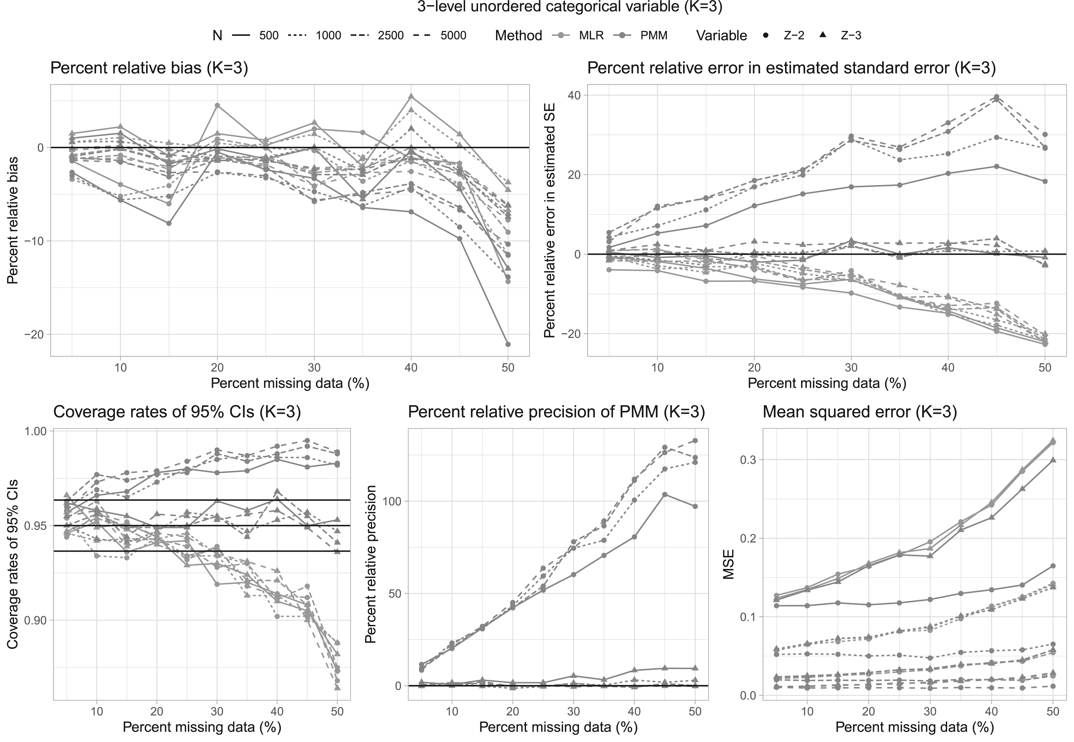Results for the two imputation methods are reported using different colors (red for multinomial logistic regression and blue for PMM), while the variable for which results are reported (the K–1 dummy variables necessary to represent Z; as described above, $Z_{j}$ represents the dummy variable used to represent the jth level of Z, with j = 2, …, K) are reported using different plotting symbols and the sample size are reported using different line types.

Figure 1.

Three-level unordered categorical variable (K = 3).

Results are also summarized in Figure 2 using boxplots. This figure has 20 panels, one for each combination of performance metric and value of K. There is one row for each of the performance metrics and one column for each of the values of K. For four of the performance metrics (percent relative bias, percent relative error in estimated standard error, empirical coverage rates of 95% confidence intervals, and MSE), we report side-by-side boxplots comparing the distribution of the performance metric across the different estimates. For K = 3, 4, 5, and 6, there are 80, 120, 160, and 200 different estimates. For K = 3, there were 80 estimated regression coefficients (40 scenarios [4 sample sizes × 10 prevalences of missing data] × two regression coefficients [the two dummy variables required to represent Z]) (with a similar calculation for the other values of K). For the fourth performance metric, percent relative precision, we report only a single boxplot for PMM, since this metric implicitly incorporates a comparison with multinomial logistic regression.

Figure 2.

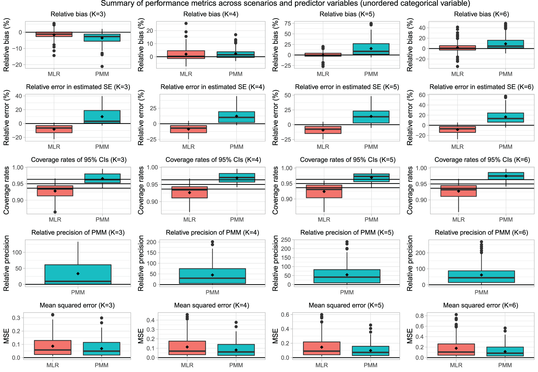
Summary of performance metrics across scenarios and predictor variables (unordered categorical variable).

The percent relative bias is reported in the top left panel of Figure 1. We have superimposed a horizontal line on this panel denoting a 0% relative bias (i.e. unbiased estimation of the regression coefficient). Bias tended to be minimal, with percent relative bias ranging from approximately −20% to ∼5%. The distribution of percent relative bias across the 80 estimated is reported in Figure 2. The two boxplots illustrate that, in general, the use of multinomial logistic regression tended to result in estimates with a negligibly lower percent relative bias. Overall, relative bias was negligible for both methods.

The percent relative error in the estimated standard errors is reported in the top right panel of Figure 1. We have superimposed a horizontal line on this panel denoting a relative percent error of zero (i.e. unbiased estimation of the standard error). Differences between the two imputation methods were more pronounced for the percent relative error in estimated standard errors than they were for the percent relative bias in estimated regression coefficients. When using PMM, the estimated standard errors for $Z_{2}$ displayed a positive relative bias (i.e. the estimated standard errors were too large) regardless of sample size and the rate of missing data. In contrast to this, the use of multinomial logistic regression tended to result in underestimation of the standard deviation of the sampling distribution, particularly as the rate of missing data increased. The distribution of percent relative error across the 80 estimated coefficients is reported using side-by-side boxplots in Figure 2. The boxplots reinforced the observations made in the previous figure, with PMM tending to result in a modest positive bias, while multinomial logistic regression tended to result in a modest negative bias.

The empirical coverage rates of estimated 95% confidence intervals are reported in the lower left panel of Figure 1. We have superimposed horizontal lines on this panel denoting empirical coverage rates of 0.9365, 0.95, and 0.9635. As noted above, empirical type I error rates that are < 0.9365 or > 0.9635 are statistically significantly different from the advertised rate of 95%. The use of PMM tended to result in estimated 95% confidence intervals whose empirical coverage rates were either not statistically significantly different from the advertised rate or that were conservative (i.e. whose empirical coverage rate was higher than the advertised rate). In contrast to this, the use of multinomial logistic regression often resulted in estimated 95% confidence intervals whose empirical coverage rates were lower than the advertised rate when the rate of missing data was high. The distribution of empirical coverage rates across the 80 estimated regression coefficients is reported using side-by-side boxplots in Figure 2. In general, the use of PMM tended to result in confidence intervals that did not differ from the advertised rate or that were conservative. In contrast to this, in ∼50% of the comparisons, multinomial logistic regression resulted in confidence intervals whose empirical coverage rates were lower than advertised.

The relative percent increase in precision for PMM compared to multinomial logistic regression is reported in the bottom middle panel of Figure 1. We have superimposed a horizontal line on this panel denoting a relative percent increase in precision of zero. The use of PMM tended to result in estimates of the regression coefficient for $Z_{2}$ that displayed greater precision (i.e. had a lower empirical standard error) compared to the use of multinomial logistic regression, whereas PMM tended to result in estimates of the regression coefficient for $Z_{3}$ that had approximately the same precision as those obtained using multinomial logistic regression. The distribution of relative percent increase in precision for PMM compared to multinomial logistic regression across the 80 estimated regression coefficients is reported in Figure 2. In general, the use of PMM tended to result in estimates that had greater precision (i.e. the empirical standard error was smaller).

The MSE of the estimated regression coefficients are reported in the lower right panel of Figure 1. In general, the MSE of the estimate obtained using PMM tended to be approximately the same as or lower than that of the estimate obtained using multinomial logistic regression. The distribution of MSE across the 80 estimated regression coefficients is reported using side-by-side boxplots in Figure 2. The boxplots confirm the above observation that the MSE when using PMM tended to be slightly lower than when using multinomial logistic regression.

4.1.1.2 Four-level categorical variable (K = 4)

Results for the 40 scenarios with K = 4 are reported in Figure 3, which has a similar structure to that of Figure 1, while the distribution of percent relative bias across 120 estimated regression coefficients is reported using side-by-side boxplots in Figure 2. Overall, the two imputation methods displayed similar relative bias across the 120 estimated regression coefficients.

Figure 3.

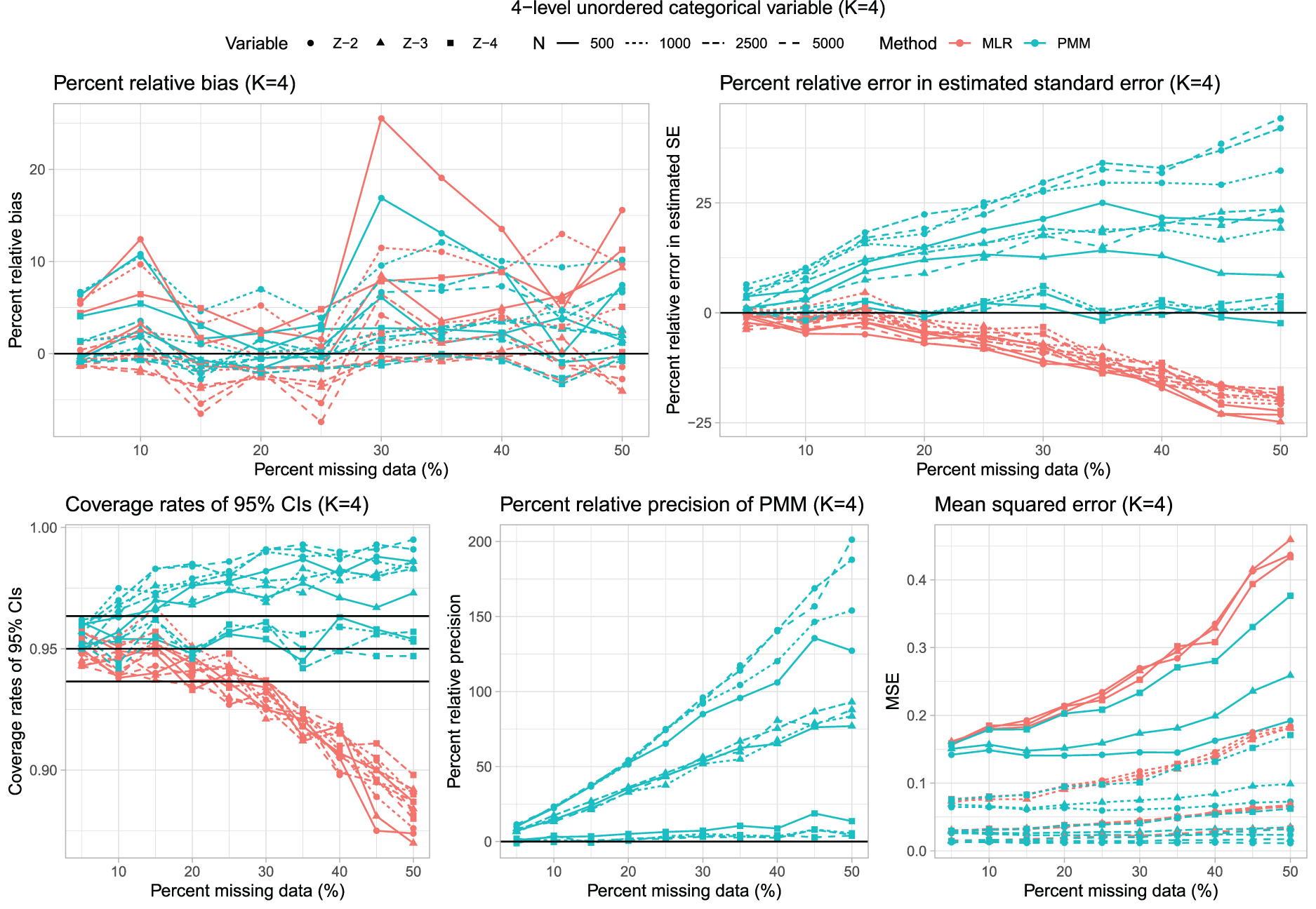
Four-level unordered categorical variable (K = 4).

The percent relative error in the estimated standard error were comparable to those observed for K = 3. The distribution of percent relative bias in the estimated standard error across the 120 estimated regression coefficients is reported in Figure 2. On average, the use of PMM resulted in a modest positive bias in the estimation of the standard error, while the use of multinomial logistic regression tended to result in minor underestimation of the standard error.

As with K = 3, the use of multinomial logistic regression often resulted in estimated confidence intervals whose empirical coverages were lower than advertised when the rate of missing data was high. This did not occur when using PMM. The distribution of empirical coverage rates across the 120 estimated regression coefficients is reported using side-by-side boxplots in Figure 2. The use of multinomial logistic regression resulted in confidence intervals whose empirical coverage rates were lower than the advertised rate in ∼50% of the instances, while this did not occur when using PMM.

The use of PMM tended to result in estimated regression coefficients that were estimated more precisely (Figure 2). Similarly, the use of PMM tended to result in estimates with lower MSE compared to when using multinomial logistic regression.

4.1.1.3 Five-level categorical variable (K = 5)

Results for scenarios with K = 5 are reported in Figure 4, which has a similar structure to that of Figures 1 and 3. In general, the use of multinomial logistic regression tended to result in estimated regression coefficients with a lower percent relative bias (Figure 2).

Figure 4.

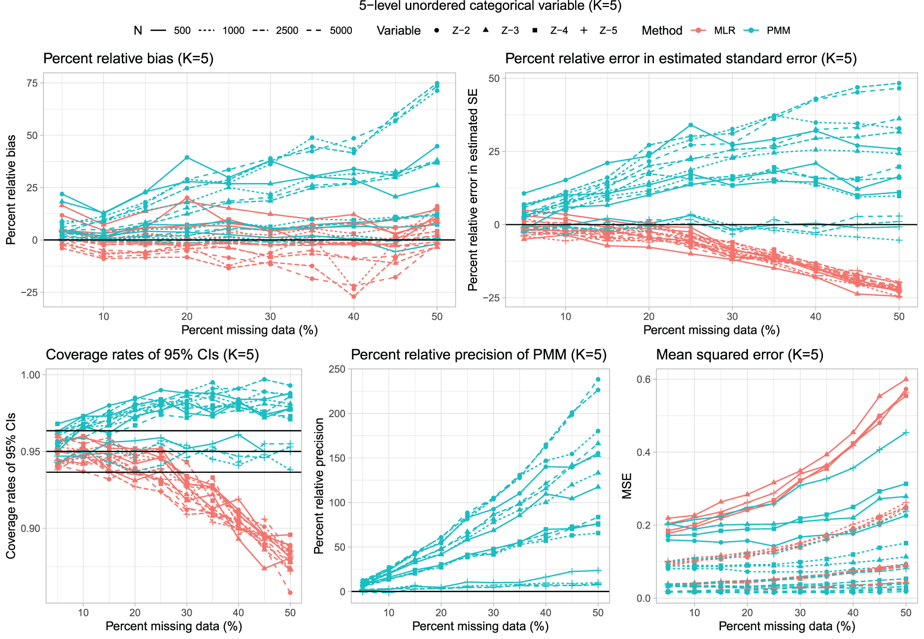
Five-level unordered categorical variable (K = 5).

The percent relative error in the estimated standard error was comparable to those observed for K = 3 and K = 4. In particular, the use of multinomial logistic regression tended to result in underestimation of the standard error when the rate of missing data was moderate to high. The distribution of percent relative error in the estimated standard error across the 160 estimated regression coefficients is reported in Figure 2. In general, the use of multinomial logistic regression tended to result in estimates that underestimated the standard deviation of the sampling distribution of the regression coefficients, while the use of PMM tended to result in estimates that overestimated the standard deviation of the sampling distribution. However, the absolute magnitude of the percent relative error tended to be smaller when using multinomial logistic regression compared to using PMM.

As with K = 3 and K = 4, multinomial logistic regression often resulted in estimated confidence intervals whose empirical coverages were lower than advertised when the rate of missing data was high. The distribution of the empirical coverage rates across the 160 estimated regression coefficients is reported in Figure 2. The use of multinomial logistic regression tended to result in confidence intervals whose empirical coverages were significantly lower than the advertised rate more frequently than did the use of PMM.

The use of PMM tended to result in estimated regression coefficients that were estimated more precisely (i.e. that had a smaller empirical standard error) compared to when multinomial logistic regression was used (Figure 2). Similarly, the use of PMM tended to result in estimated regression coefficients that had lower MSE compared to when multinomial logistic regression was used.

4.1.1.5 6-level categorical variable (K = 6)

Results for scenarios with K = 6 are reported in Figure 5, which has a structure similar to Figures 1, 3 and 4. The distribution of percent relative bias across the 200 estimated regression coefficients is reported using side-by-side boxplots in Figure 2. The use of PMM tended to result in estimates with modestly more bias than when using multinomial logistic regression.

Figure 5.

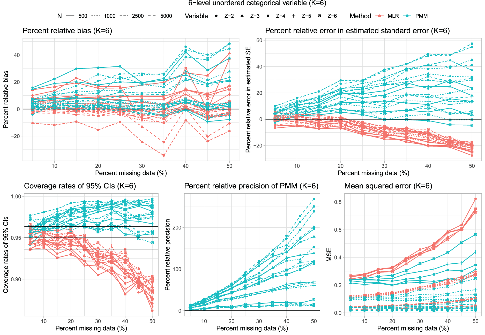
Six-level unordered categorical variable (K = 6).

Multinomial logistic regression tended to result in modest underestimation of the standard error when the rate of missing data was moderate to high. In contrast to this, the use of PMM tended to result in estimates of standard errors that were biased upwards.

As with K = 3, K = 4, and K = 5, the use of multinomial logistic regression often resulted in estimated confidence intervals whose empirical coverages were lower than advertised when the rate of missing data was high. This did not occur when using PMM. In examining the side-by-side boxplots in Figure 2, one observes that in ∼50% of the instances, the use of multinomial logistic regression resulted in estimated confidence intervals whose empirical coverages were statistically significantly lower than advertised.

Finally, as with the other values of K, the use of PMM tended to result in estimated regression coefficients that had smaller empirical standard errors. Similarly, the use of PMM tended to result in estimates with lower MSE compared to when multinomial logistic regression was used.

4.1.2 Ordinal categorical variable

The simulations took 352.6 h (14.7 days) when using ordinal logistic regression to impute the K-level categorical variable and 100.7 h (4.2 days) when using PMM. Thus, the use of ordinal logistic regression required ∼3.5 times more time than the use of PMM.

Results for ordinal categorical variables are reported in Figures 6 to 10, which have structures identical to those of Figures 1 to 5. We briefly summarize the results, focusing on Figure 7, which uses boxplots to summarize the distribution of the performance metrics across the different combinations of scenarios and estimated regression coefficients.

Figure 6.

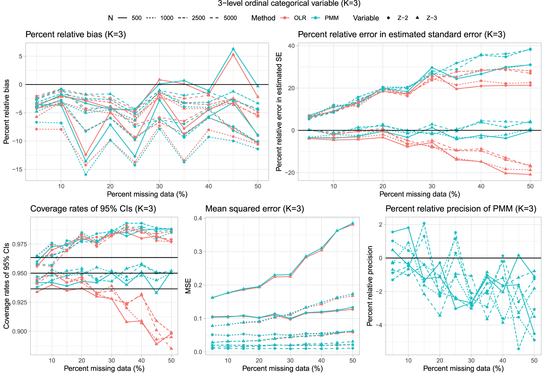
Three-level ordinal categorical variable (K = 3).

Figure 7.

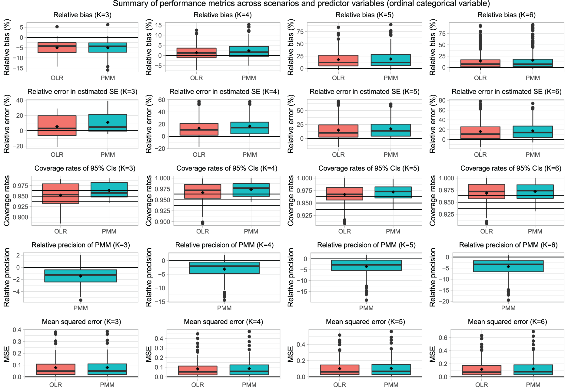
Summary of performance metrics across scenarios and predictor variables (ordinal categorical variable).

Figure 8.

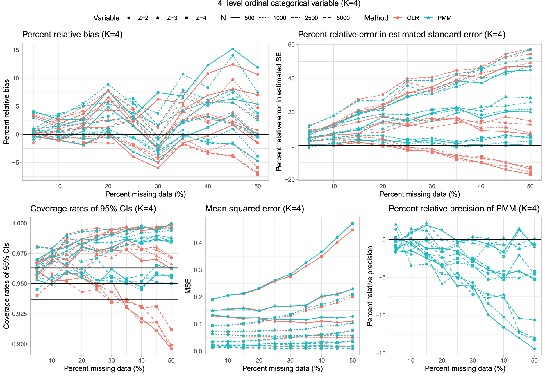
Four-level ordinal categorical variable (K = 4).

Figure 9.

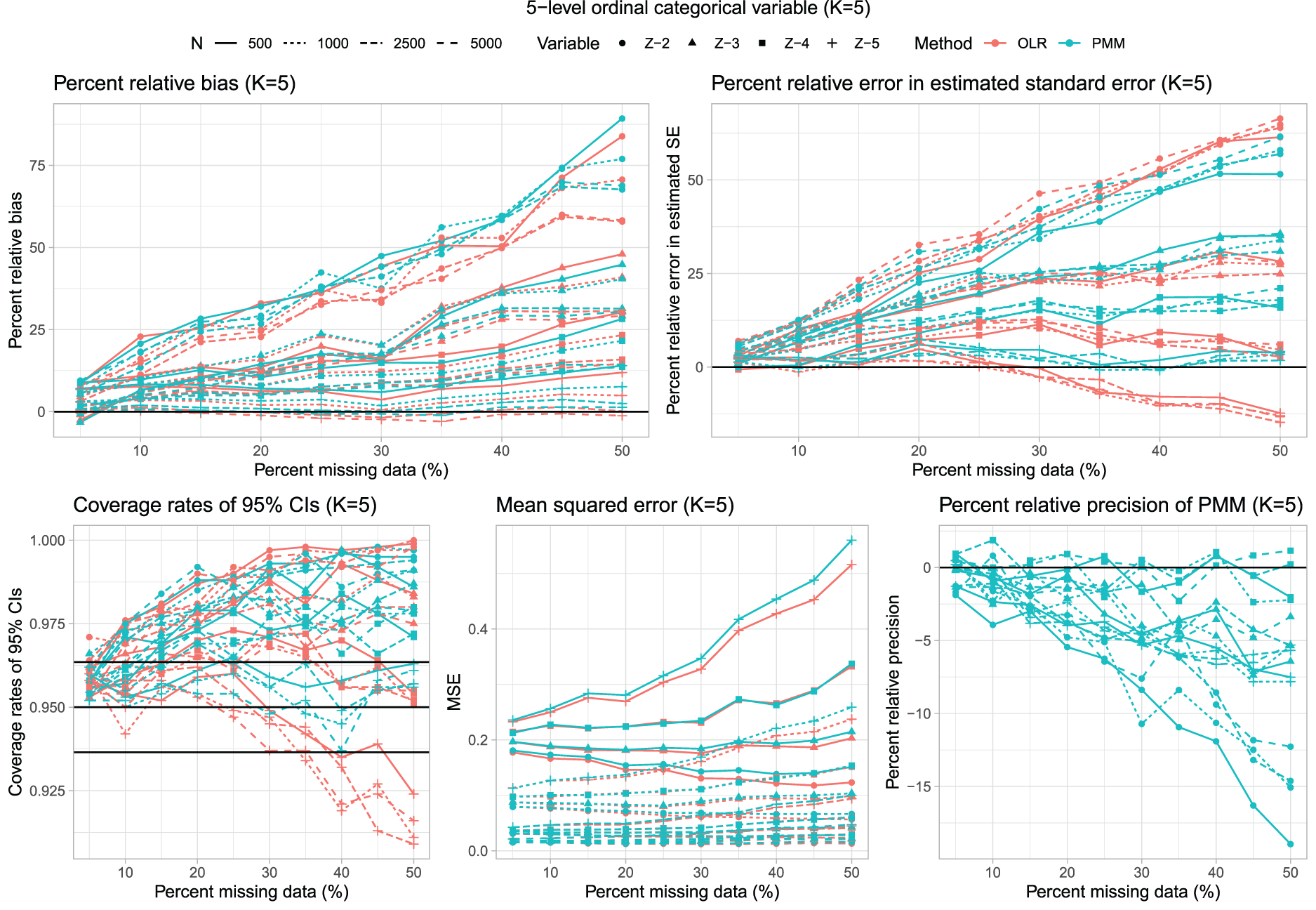
Five-level ordinal categorical variable (K = 5).

Figure 10.

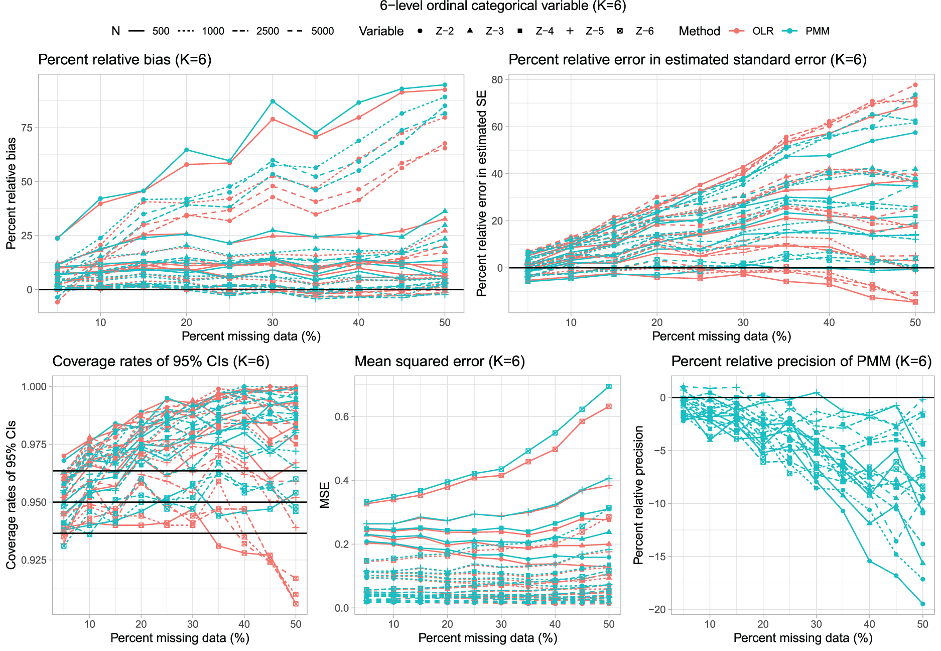
Six-level ordinal categorical variable (K = 6).

When assessed using the percent relative bias in the estimated regression coefficients, differences between the use of ordinal logistic regression and PMM tended to be minimal. On average, differences between the two methods were negligible. Similarly, differences between ordinal logistic regression and PMM when estimating standard errors of the estimated regression coefficients tended, on average, to be minimal.

The use of ordinal logistic regression resulted in estimated 95% confidence intervals whose empirical coverages were statistically significantly lower than the advertised rate in a modest number of scenarios. In contrast to this, in almost all the scenarios, the use of PMM resulted in 95% confidence intervals whose empirical coverage rates were either not significantly different from the advertised rate or that were conservative (i.e. higher than the advertised rate).

In contrast to what was observed with the nominal categorical variable, the use of PMM resulted in estimated regression coefficients that were less precise than those obtained when using ordinal logistic regression. However, the decrease in imprecision tended to be negligible to modest in most scenarios. Finally, the choice of imputation algorithm tended to have a negligible impact on the MSE of the estimated regression coefficients.

4.2 Analysis model was a linear regression model

When the categorical variable was nominal, the simulations took 323.6 h (13.5 days) when using multinomial logistic regression to impute the K-level categorical variable and 62.5 h (2.6 days) when using PMM. Thus, the use of multinomial logistic regression required ∼5.2 times more time than the use of PMM. When the categorical variable was ordinal, the simulations took 355.2 h (14.8 days) when using multinomial logistic regression to impute the K-level categorical variable and 59.4 h (2.5 days) when using PMM. Thus, the use of multinomial logistic regression required ∼6 times more time than the use of PMM.

The results of the simulations are summarized in Supplemental Figures A1 to A10. These 10 figures have a structure identical to those of Figures 1 to 10. Overall, the results on the quality of statistical inferences were similar to those observed in the settings in which the analysis model was a logistic regression model.

5. Discussion

We evaluated the performance of PMM in comparison to multinomial logistic regression (for imputing nominal categorical variables) and ordinal logistic regression (for imputing ordinal categorical variables). Performance was assessed in settings where the analysis model was either a logistic or a linear regression model. Overall, PMM performed comparably, or even favorably, to both logistic and ordinal regression in terms of inference quality, while requiring substantially less computational time. Across simulation scenarios, PMM was about 3 to 6 times faster than parametric models, highlighting its practical advantage for large-scale or high-dimensional applications.

One reason for PMM's superior speed is that it avoids the problem of perfect prediction, which often complicates logistic regression models and may require artificially adding regularization records. Instead of relying on iterative likelihood maximization, PMM uses ordinary least squares within a linear modeling framework, which is simpler and faster to compute. Moreover, the mice package implementation of PMM leverages optimized C routines for efficiently generating donor-based imputations.

The strong performance of PMM for imputing missing categorical data can be attributed to the similarity between the linear predictors used in linear and logistic regression models, particularly in the central part of the outcome distribution. PMM handles categorical variables by applying an optimal scaling transformation that assigns numeric values to each category, effectively converting the outcome into a quasi-continuous variable. For ordinal variables, this transformation can be constrained to follow a monotonic pattern that respects the category order, which may enhance stability when the ordinal structure is correctly specified. However, imposing such constraints risks introducing systematic bias if the assumed order is incorrect. To avoid this, we recommend not enforcing monotonicity by default. A practical benefit of this choice is that PMM remains invariant to the ordering of categories.

From a practical standpoint, PMM emerges as a competitive and pragmatic default for the imputation of categorical variables. Not only does it match the inferential performance of parametric alternatives, but it also completes imputations in roughly one-third to one-sixth of the time. Its non-parametric nature also allows it to capture certain kinds of nonlinearity that standard logistic models may fail to capture.

Nonetheless, caution is warranted in specific settings. PMM can be less stable in regions with sparse outcome data, such as tails or gaps, where the behavior of the linear predictor becomes erratic. For applications requiring robust extrapolation or precise modeling of extremes, parametric models are preferable. Additionally, some categorical structures may not linearize well. In such cases, extending the approach to allow for multiple orthogonal quantifications of the outcome (i.e. using a multivariate representation) may improve robustness and capture complex patterns.

The current study is subject to certain limitations. First, our study relied on Monte Carlo simulations. Consequently, our findings are dependent on the data-generating process that was used. It is possible that PMM may have inferior performance compared to the use of multinomial or ordinal logistic regression in other settings. We suggest that our methods be replicated in other settings to examine the generalizability of our findings. Second, we did not include an examination of the complete case estimator, which is often included in studies examining the performance of MI-based estimators. The rationale for this omission was that we were motivated by examining whether PMM could be used instead of multinomial or ordinal logistic regression for imputing missing categorical variables. We were not interested in comparing how each imputation method compared with the use of a complete case analysis.

In conclusion, PMM offers a fast, flexible, and statistically sound alternative to conventional multinomial and ordinal regression models for imputing categorical data. Its combination of computational efficiency and favorable inferential properties makes it a strong candidate for default use in the mice framework and other MI workflows.

Supplemental Material

sj-pdf-1-smm-10.1177_09622802251362642 - Supplemental material for Imputation of incomplete ordinal and nominal data by predictive mean matching

Supplemental material, sj-pdf-1-smm-10.1177_09622802251362642 for Imputation of incomplete ordinal and nominal data by predictive mean matching by Peter C Austin and Stef van Buuren in Statistical Methods in Medical Research

Footnotes

Declaration of conflicting interests

The author(s) declared no potential conflicts of interest with respect to the research, authorship, and/or publication of this article.

Funding

ICES is an independent, non-profit research institute funded by an annual grant from the Ontario Ministry of Health (MOH) and the Ministry of Long-Term Care (MLTC). As a prescribed entity under Ontario's privacy legislation, ICES is authorized to collect and use health care data for the purposes of health system analysis, evaluation, and decision support. Secure access to these data is governed by policies and procedures that are approved by the Information and Privacy Commissioner of Ontario. This study was supported by ICES, which is funded by an annual grant from the Ontario Ministry of Health (MOH) and the Ministry of Long-Term Care (MLTC). This study also received funding from the Canadian Institutes of Health Research (CIHR) (PJT 166161). This document used data adapted from the Statistics Canada Postal CodeOM Conversion File, which is based on data licensed from Canada Post Corporation, and/or data adapted from the Ontario Ministry of Health Postal Code Conversion File, which contains data copied under license from ^©Canada Post Corporation and Statistics Canada. Parts of this material are based on data and/or information compiled and provided by CIHI and the Ontario Ministry of Health. The analyses, conclusions, opinions, and statements expressed herein are solely those of the authors and do not reflect those of the funding or data sources; no endorsement is intended or should be inferred. The dataset from this study is held securely in coded form at ICES. While legal data sharing agreements between ICES and data providers (e.g. healthcare organizations and government) prohibit ICES from making the dataset publicly available, access may be granted to those who meet pre-specified criteria for confidential access, available at (email: das@ices.on.ca).

Supplementary material

Supplementary material for this paper is available online.

ORCID iD

Peter C Austin

References

Rubin

. Multiple imputation for nonresponse in surveys. New York: John Wiley & Sons, 1987.

van Buuren

. Flexible imputation of missing data. Second edition. Boca Raton, FL: CRC Press, 2018.

White

Royston

Wood

. Multiple imputation using chained equations: issues and guidance for practice. StatMed 2011; 30: 377–399.

van Buuren

. Multiple imputation of discrete and continuous data by fully conditional specification. Stat Methods Med Res 2007; 16: 219–242.

van Buuren

Groothuis-Oudshoorn

. mice: multivariate imputation by chained equations in R. J Stat Softw 2011; 45: 1–67.

White

Daniel

Royston

. Avoiding bias due to perfect prediction in multiple imputation of incomplete categorical variables. Comput Stat Data Anal 2010; 54: 2267–2275.

Austin

van Buuren

. Logistic regression vs. predictive mean matching for imputing binary covariates. Stat Methods Med Res 2023; 32: 2172–2183.

Gifi

. Nonlinear multivariate analysis. New York, NY: John Wiley & Sons, 1990.

de Leeuw

Young

Takane

. Additive structure in qualitative data: an alternating least squares method with optimal scaling features. Psychometrika 1976; 41: 471–503.

10.

Breiman

Friedman

. Estimating optimal transformations for multiple regression and correlation. J Am Stat Assoc 1985; 80: 580–598.

11.

Harrell

. Hmisc: Harrell miscellaneous [computer program]. Version R package version 5.2-32025. http://CRAN.R-project.org/package=Hmisc

12.

Donovan

Lee

, et al. Effectiveness of public report cards for improving the quality of cardiac care: the EFFECT study: a randomized trial. J Am Med Assoc 2009; 302: 2330–2337.

13.

Barnard

Rubin

. Small-sample degrees of freedom with multiple imputation. Biometrika 1999; 86: 948–955.

14.

Morris

White

Royston

. Tuning multiple imputation by predictive mean matching and local residual draws. BMC Med Res Methodol 2014; 14: 75.

15.

Morris

White

Crowther

. Using simulation studies to evaluate statistical methods. Stat Med 2019; 38: 2074–2102.

16.

Gasparini

. Rsimsum: summarise results from Monte Carlo simulation studies. J Open Source Softw 2018; 3: 739.

Supplementary Material

Please find the following supplemental material available below.

For Open Access articles published under a Creative Commons License, all supplemental material carries the same license as the article it is associated with.

For non-Open Access articles published, all supplemental material carries a non-exclusive license, and permission requests for re-use of supplemental material or any part of supplemental material shall be sent directly to the copyright owner as specified in the copyright notice associated with the article.

0.00 MB

0.24 MB