Unit information prior for incorporating real-world evidence into randomized controlled trials

Abstract

Randomized controlled trials (RCTs) have been widely recognized as the gold standard to infer the treatment effect in clinical research. Recently, there has been growing interest in enhancing and complementing the result in an RCT by integrating real-world evidence from observational studies. The unit information prior (UIP) is a newly proposed technique that can effectively borrow information from multiple historical datasets. We extend this generic approach to synthesize the non-randomized evidence into a current RCT. Not only does the UIP only require summary statistics published from observational studies for ease of implementation, but it also has clear interpretations and can alleviate the potential bias in the real-world evidence via weighting schemes. Extensive numerical experiments show that the UIP can improve the statistical efficiency in estimating the treatment effect for various types of outcome variables. The practical potential of our UIP approach is further illustrated with a real trial of hydroxychloroquine for treating COVID-19 patients.

1 Introduction

Randomized controlled trials (RCTs) are widely recognized as the gold standard to evaluate the efficacy of a treatment in clinical studies. However, the rigorous experimental settings and inclusion criteria restrict the generalisability of trial results to the routine clinical practice. ¹ It is also costly and slow for RCTs to deliver the findings if a large number of subjects are required to be followed for a long period of time. In order to complement and enhance the evidence in an RCT, information synthesis from the ubiquitous real-world evidence or observational studies into therapeutic development has recently received growing attention in the medical literature.^2–4 Motivated by the above concerns, a variety of statistical methods have been proposed to integrate the non-randomized and randomized evidence, most of which are based on the Bayesian framework due to its prominent flexibility in combining multi-source information. When only aggregate data are available for both RCTs and observational studies, the real-world evidence is typically quantified using meta-analysis techniques,^5–8 such as through the prior distribution of the treatment effect parameter in a network meta-analysis model, or through a multi-level Bayesian hierarchical model. The aforementioned methods are typically designed for aggregating the published summary statistics from all studies, including the treatment effect estimates with the corresponding standard errors, and thus they cannot be directly applied to the scenario where the individual patient data are available for a current RCT.

For the cases where investigators have access to patient-level data of both randomized and non-randomized studies, many approaches have been proposed for evidence synthesis following the idea of propensity scores. ⁹ Lin et al.^10,11 leveraged the observational samples to augment the disproportionate RCT into a 1:1 randomized trial, and then discounted the borrowed samples via propensity score-based priors. Wang et al. ¹² proposed a Bayesian nonparametric approach to jointly modeling the outcomes and the corresponding propensity scores from different types of studies. Liu et al. ¹³ introduced a stratum-specific meta-predictive-analytic prior to including the observational evidence following propensity scores. A three-stage framework was proposed to validate observational data with the RCT as an anchor and integrate the statistical evidence from both sources. ¹⁴ Although the individual patient data could allow flexible and effective synthesis of information, they are difficult to obtain for all observational studies in practice while typically only summary statistics are available in the published literature.

We hence focus on the situation where the investigator needs to infer the treatment effect from the patient-level data of a current RCT, while additional summary statistics can be obtained from publications of related observational studies to enhance the RCT results. We assume that the causal estimands are the same between the RCT and observational studies, such as the hazard ratio or odds ratio. This scenario is particularly common under the current COVID-19 pandemic, because the urgency of health care has promoted numerous observational analyses prior to the report released from a well-conducted RCT.^15,16 Some attempts have been made in the literature to deal with the synthesis for mixed data that consist of individual patient data and aggregate information, such as the simulated treatment comparison, ¹⁷ matching-adjusted indirect comparisons, ¹⁸ Bayesian aggregation ¹⁹ and Bayesian meta-analysis with individual data.^20,21 However, those approaches are either only applicable to some specific types of outcomes,^20,21 not pertinent to our scenario,^17,16,19 or unable to account for the potential bias of observational evidence caused by heterogeneity and confounding effects. ²⁰ Recently, Jin and Yin ²² proposed the unit information prior (UIP) to borrow evidence from historical studies. This approach has several salient advantages to address the information synthesis in our scenario. First, the UIP only requires summary statistics of the historical trials, which is common in the published literature. Second, the UIP can account for the heterogeneity between the current and historical datasets through an appropriate weighting scheme, which helps to discount the biased information.^5,6 Furthermore, it automatically determines the amount of information for integration from different historical datasets. Finally, this method is generic and can be readily modified to accommodate various types of outcomes. However, Jin and Yin ²² focused on the development of UIP for binary and continuous data from historical RCTs rather than observational studies. It is thus of great interest to explore the application of this method to incorporate the historical observational evidence into a current RCT with the availability of individual patient data involving various covariates and different types of outcomes. Particularly, we construct the UIP for the causal parameter of treatment effect using the point estimators from the observational studies with their standard errors, which are invariant to the types of outcome variables. We further evaluate the performance of UIP on continuous, binary, and time-to-event outcomes under different configurations.

The remainder of this article is organized as follows. Section 2 introduces how the real-world evidence can be incorporated using the UIP in the estimation of the parameter of interest in an RCT. We present the settings and results of comprehensive numerical experiments in Section 3, where we find that UIP can effectively improve the statistical efficiency of estimation. In Section 4, we re-analyze a randomized trial of hydroxychloroquine for treating COVID-19 by synthesizing the evidence from several observational studies. We conclude with a brief discussion in Section 5.

2 Methodology

2.1 Problem formulation

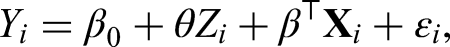
Let $\mathbf{X}=({\mathbf{X}}_1,\dots ,{\mathbf{X}}_n{)}^{\mathrm{\top }}\in {\mathbb{R}}^{n\times d}$ denote the covariate matrix for $n$ enrolled patients in a current RCT. We assume that the RCT only involves one treatment and one control arm, and accordingly let $Z=(Z_1,\dots ,Z_n{)}^{\mathrm{\top }}$ be the binary allocation indicators with $Z_i\in \{0,1\}$ for $i=1,\dots ,n$ . The $i$ th patient is assigned to the treatment arm if $Z_i=1$ and to the control arm otherwise. The allocation variable $Z_i$ is generated from randomization. The outcome variables $\mathbf{Y}=(Y_1,\dots ,Y_n{)}^{\mathrm{\top }}\in {\mathbb{R}}^n$ are then collected based on the treatment assignment. Our methodology is general enough to consider different types of outcomes, including continuous, binary, and survival data. For the survival outcome, the variable $Y_i$ refers to the observed follow-up time under an independent right-censoring assumption. We additionally observe the event indicators $\delta =({\delta }_1,\dots ,{\delta }_n{)}^{\mathrm{\top }}$ with ${\delta }_i\in \{0,1\}$ for the survival outcome, where we have ${\delta }_i=1$ if the event occurs otherwise ${\delta }_i=0$ indicating that $Y_i$ is a censored observation. We thus have the individual patient data $\mathcal{D}=\{\mathbf{Y},\mathbf{Z},\mathbf{X},\delta \}$ for the current RCT data, where $\delta$ is fixed as a vector of 1s denoted by $\mathbf{1}$ (i.e. no censoring) under continuous and binary outcomes for convenience.

Given the observed RCT data $\mathcal{D}$ , we consider a general modeling structure that can cover different types of outcomes

$$P(Y_i|X_i,Z_i,{\delta }_i)=f(Y_i,{\delta }_i,{\beta }_0+\theta Z_i+{\beta }^{\mathrm{\top }}{X}_i),$$

(1)

which denotes the probabilistic model for treatment inference with ${\beta }_0$ , $\theta$ , and $\beta$ as parameters for the linear predictor. The function $f(\cdot )$ is specified accordingly depending on the type of outcome $Y$ . For the continuous outcome, we adopt a linear model

$$Y_i={\beta }_0+\theta Z_i+{\beta }^{\mathrm{\top }}{\mathbf{X}}_i+{\epsilon }_i,$$

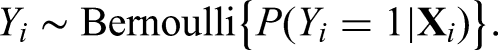
where ${\epsilon }_i\sim N(0,{\sigma }_{\epsilon }^2)$ and ${\sigma }_{\epsilon }^2$ is the unknown variance. For the binary outcome, the logistic regression is considered with

$$\text{logit}\{P(Y_i=1|{\mathbf{X}}_i)\}={\beta }_0+\theta Z_i+{\beta }^{\mathrm{\top }}{\mathbf{X}}_i.$$

As for the survival outcome, we use the Cox proportional hazards model with the hazard function $h(t|Z_i,{\mathbf{X}}_i)$ defined as

$$h(t|Z_i,{\mathbf{X}}_i)=h_0(t)\exp (\theta Z_i+{\beta }^{\mathrm{\top }}{\mathbf{X}}_i),$$

where $h_0(t)$ is the unknown baseline hazard function. The parameter $\theta$ or its transformation is related to the treatment effect of interest, which represents the additive treatment effect for the continuous outcome, the odds ratio (OR) for the binary outcome, and the hazard ratio (HR) for the survival outcome. The parameter ${\beta }_0$ corresponds to the intercept under the linear and logistic models and $\beta$ represents the coefficient vector for covariate effects. Our major goal is to make a comprehensive estimation of $\theta$ by synthesizing $\mathcal{D}$ and aggregate evidence from observational studies. Before the formal integration analysis is carried out, we should collect all the necessary aggregate data from relevant observational studies.

2.2 Aggregate data from observational studies

Suppose that we have $K$ historical observational studies that are closely related to the current RCT. There are several fundamental criteria for selecting appropriate observational studies to be included in our synthesis analysis. First, all observational studies should conceptually consider the same clinical objective and intervention as the current RCT, and numerically adopt the same parameter to measure the treatment effect. For example, both observational studies and the current RCT use the HR for survival data to measure the treatment effect. Second, the study design of observational data should be similar to the RCT for controlling the heterogeneity among studies, for example, the inclusion criteria are similar so that participants should have a comparable range of ages and symptoms. Finally, we require that all covariates should be balanced for the estimation of treatment effect in these observational studies to reduce the bias caused by confounding effects. Typically, this refers to analysis based on propensity scores, such as through matching ²³ or weighting ²⁴ schemes, which has been widely adopted for analyzing observational data in the medical research.^25,26 All information for checking the criteria can be readily found in the abstract of medical publications.

Let ${\theta }_k$ denote the parameter of treatment effect in the $k$ th observational study for $k=1,\dots ,K$ , which is the counterpart of $\theta$ in the current RCT. We only require three summary statistics for ${\theta }_k$ from each observational study. First, we should obtain the maximum likelihood estimator (MLE) ${\hat{\theta }}_k$ for ${\theta }_k$ and the corresponding standard error $SE({\hat{\theta }}_k)$ . For binary and survival outcomes, ${\hat{\theta }}_k$ is obtained by conducting the logarithmic transformation on OR and HR, respectively. The standard error can be derived from the confidence interval (CI) if it is not directly provided in the published literature. Assume that the 95% CI is $[l_k,u_k]$ for the $k$ th study, and we can calculate the standard error by $SE({\hat{\theta }}_k)=\{g(l_k)-g(u_k)\}/(2\times 1.96)$ , where $g(\cdot )$ is a transformation function based on the type of outcomes. For example, we have $g(\cdot )=\log (\cdot )$ if $\exp ({\theta }_k)$ corresponds to OR or HR. Sometimes, the published medical papers may provide multiple estimators for ${\theta }_k$ based on different covariate-balancing approaches, ²⁷ while we only adopt the results from the primary analysis for integration. Second, we need the corresponding sample size $n_k$ used in the primary analysis, which should be distinguished from the original sample size in the observational study. For instance, we should specify $n_k$ as the sample size of matched data if the primary analysis uses a matching method to balance covariates. We use ${\mathcal{S}}_k=\{{\hat{\theta }}_k,SE({\hat{\theta }}_k),n_k\}$ to denote the summary information in the primary analysis of the $k$ th observational study. After collecting ${\mathcal{S}}_1,\dots ,{\mathcal{S}}_K$ , we can construct the UIP and then conduct Bayesian inference for $\theta$ in the current RCT.

2.3 Unit information prior

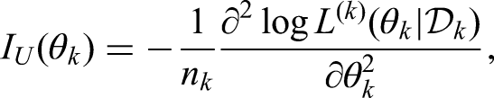
Let ${\mathcal{D}}_k$ denote the underlying individual patient data corresponding to ${\mathcal{S}}_k$ , and $L^{(k)}({\theta }_k|{\mathcal{D}}_k)$ refers to the likelihood function for ${\theta }_k$ . According to Jin and Yin, ²² we first introduce the unit information $I_U({\theta }_k)$ for ${\theta }_k$ ,

$$I_U({\theta }_k)=-\frac{1}{n_k}\frac{{\mathrm{\partial }}^2\log L^{(k)}({\theta }_k|{\mathcal{D}}_k)}{\mathrm{\partial }{\theta }_k^2},$$

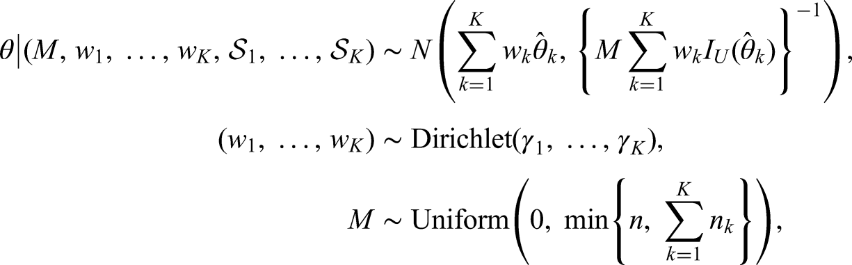
which represents the observed Fisher information at a unit sample level. The UIP to $\theta$ in the current RCT is then defined as follows:

$$\begin{array}{rl}\theta |(M,w_1,\dots ,w_K,{\mathcal{S}}_1,\dots ,{\mathcal{S}}_K)& \sim N(\sum _{k=1}^K{w}_k{\hat{\theta }}_k,{\{M\sum _{k=1}^K{w}_k{I}_U({\hat{\theta }}_k)\}}^{-1}),\\ (w_1,\dots ,w_K)& \sim \text{Dirichlet}({\gamma }_1,\dots ,{\gamma }_K),\\ M& \sim \text{Uniform}(0,min\{n,\sum _{k=1}^K{n}_k\}),\end{array}$$

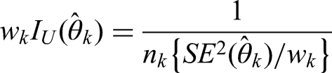
where $I_U({\hat{\theta }}_k)$ refers to the unit information evaluated at ${\hat{\theta }}_k$ , and $({\gamma }_1,\dots ,{\gamma }_K)$ are pre-specified hyper-parameters with ${\gamma }_k=min(1,n_k/n)$ so that a study with a larger sample size would be assigned a higher prior weight. We tend to assign a smaller weight in the Dirichlet prior for the dataset whose sample size is smaller than that of the RCT, and otherwise, the prior weight is bounded by 1. Intuitively, the UIP first incorporates the unit-level information from each observational study through the weight parameters $w_k$ , and then figures out the total amount of information to be synthesized through the parameter $M$ . Closely related to the effective sample size in the prior, ²⁸ $M$ is bounded by the sample size of the RCT $(n)$ as well as the total sample size of matched data in the observational studies $(\sum _{k=1}^K{n}_k)$ , because the UIP should not dominate the current RCT. Both $M$ and $w_k$ ’s are adaptively determined by the commensurability between the RCT and observational studies.

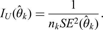
The only concern now is to specify $I_U({\hat{\theta }}_k)$ for the $k$ th observational study. Jin and Yin ²² suggested performing a case-by-case derivation to obtain the explicit form of $I_U({\hat{\theta }}_k)$ based on the type of outcome and the corresponding model. By contrast, we provide a more general alternative to determine the unit information. Following the asymptotic normality of the MLE, we have

$$\sqrt{n_k}({\hat{\theta }}_k-{\theta }_k)\to N(0,1/\mathbb{E}\{I_U({\theta }_k)\}),$$

where the expectation is taken over the distribution that generates independent individual samples in ${\mathcal{D}}_k$ . The above property shows that the asymptotic variance of ${\hat{\theta }}_k$ is $1/[n_k\mathbb{E}\{I_U({\theta }_k)\}]$ , and it thus motivates us to define $I_U({\hat{\theta }}_k)$ using the empirical standard error of ${\hat{\theta }}_k$

$$I_U({\hat{\theta }}_k)=\frac{1}{n_{k}S{E}^2({\hat{\theta }}_k)}.$$

Finally, we adopt non-informative prior (NIP) for the other parameters specified in model (1) and then perform Bayesian inference.

There are several advantages of incorporating real-world evidence using UIP. First, we only need the summary statistics ${\mathcal{S}}_k$ to construct the prior without the need for access to the individual data ${\mathcal{D}}_k$ . Second, the specification of UIP is independent of the outcome model, which greatly facilitates its broad applicability. Most importantly, the UIP accounts for the potential bias in each observational study by a weighting scheme. Different from RCTs, the estimator obtained from an observational study cannot avoid the bias that originates from the non-randomized treatment allocation, although the bias can be reduced by some post-hoc balancing techniques. Furthermore, the bias may also originate from the heterogeneity between observational studies and the current RCT. Therefore, properly discounting the observational evidence plays an essential role in the synthesis to adjust the possible over-estimation or under-estimation of the treatment effect.^5–7 In the UIP, we have

$$w_k{I}_U({\hat{\theta }}_k)=\frac{1}{n_k\{S{E}^2({\hat{\theta }}_k)/w_k\}}$$

for each study, where $w_k\in (0,1)$ inflates the standard error $S{E}^2({\hat{\theta }}_k)$ to alleviate the underlying unamendable bias. A larger weight $w_k$ leads to a smaller standard error $S{E}^2({\hat{\theta }}_k)/w_k$ , which leads to more information borrowing through the UIP.

3 Simulation

In the simulation, we evaluate the performance of the aforementioned UIP in estimating the treatment effect for the current RCT with respect to different types of outcomes. Individual patient data are first simulated for both the RCT and observational studies, and the propensity score analysis is performed on the observational data to generate the summary statistics for further synthesis.

3.1 Continuous outcome

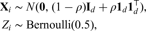
For continuous outcomes, we fix the sample size of the current RCT at $n=200$ , and generate the covariates ${\mathbf{X}}_i$ and allocation indicator $Z_i$ for the $i$ th sample $(i=1,\dots ,n)$ as follows:

$$\begin{array}{rl}{\mathbf{X}}_i& \sim N(\mathbf{0},(1-\rho ){\mathbf{I}}_d+\rho {\mathbf{1}}_d{\mathbf{1}}_d^{\mathrm{\top }}),\\ Z_i& \sim \text{Bernoulli}(0.5),\end{array}$$

where we set the correlation coefficient $\rho =0.1$ and the covariate dimension $d=6$ . The first two covariates ( $X_{ij},j=1,2$ ) are then dichotomized to 1 if it is non-negative and to 0 otherwise. Given the covariates ${\mathbf{X}}_i$ and the assignment indicators $Z_i$ , we generate the outcome variables $Y_i$ of RCT through a linear model,

$$Y_i=1+\theta Z_i+{\beta }^{\mathrm{\top }}{\mathbf{X}}_i+{\epsilon }_i,$$

where $\theta =1$ , $\beta ={\mathbf{1}}_d$ , and ${\epsilon }_i\sim N(0,{0.5}^2)$ .

For the evidence from observational studies, we consider $K=3$ historical observational studies and fix the sample size $N_k=500$ for the $k$ th study with $k=1,2,3$ . It is worth emphasizing that $N_k$ is the original sample size of the observational studies and $n_k$ in the UIP is the sample size after matching the propensity scores to balance the covariates, so $n_k\le N_k$ . Similarly, we first generate the covariates from a normal distribution with $d_k=6$ ,

$${\mathbf{X}}_i^{(k)}\sim N({\mu }_k{\mathbf{1}}_{d_k},{\sigma }_k^2(1-{\rho }_k){\mathbf{I}}_{d_k}+{\sigma }_k^2{\rho }_k{\mathbf{1}}_{d_k}{\mathbf{1}}_{d_k}^{\mathrm{\top }}),$$

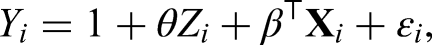
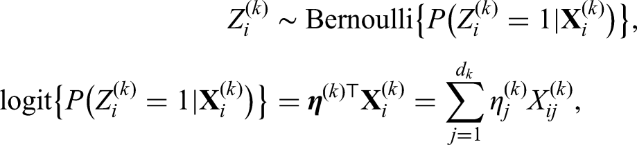
where ${\mu }_k$ and ${\sigma }_k^2$ are the covariate mean and variance, respectively, and ${\rho }_k$ denotes the correlation coefficient. The first two covariates ( $X_{ij}^{(k)},j=1,2$ ) are then dichotomized to 1 if its value is larger than ${\mu }_k$ and to 0 otherwise. For the observational studies, the treatment indicator variables depend on covariates or confounders, which are generated from the following model:

$$\begin{array}{rl}{Z}_i^{(k)}& \sim \text{Bernoulli}\{P(Z_i^{(k)}=1|{\mathbf{X}}_i^{(k)})\},\\ \text{logit}\{P(Z_i^{(k)}=1|{\mathbf{X}}_i^{(k)})\}& ={\mathit{\eta }}^{(k)\mathrm{\top }}{\mathbf{X}}_i^{(k)}=\sum _{j=1}^{d_k}{\eta }_j^{(k)}{X}_{ij}^{(k)},\end{array}$$

where $P(Z_i^{(k)}=1|{\mathbf{X}}_i^{(k)})$ is the propensity score with the coefficient vector ${\eta }^{(k)}=({\eta }_1^{(k)},\dots ,{\eta }_{d_k}^{(k)}{)}^{\mathrm{\top }}$ . After collecting the covariate matrix and the allocation indicators, we generate the continuous outcome for the $k$ th observational study via

$$Y_i^{(k)}=1+{\theta }_k{Z}_i^{(k)}+{\beta }^{(k)\mathrm{\top }}{\mathbf{X}}_i^{(k)}+{\epsilon }_i,$$

where ${\epsilon }_i\sim N(0,{0.5}^2)$ , ${\theta }_k$ and ${\beta }^{(k)}$ are the parameters of the treatment effect and covariate coefficients, respectively.

3.2 Binary outcome

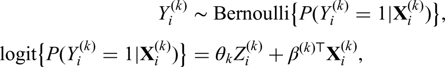
Regarding binary outcomes, the covariates and treatment indicators of the RCT and three observational studies are generated following the same procedure as that for continuous outcomes. Under a logistic model

$$\text{logit}\{P(Y_i=1|{\mathbf{X}}_i)\}=\theta Z_i+{\beta }^{\mathrm{\top }}{\mathbf{X}}_i,$$

with the coefficients $\beta =0.1\times {\mathbf{1}}_d$ , the outcome of RCT is then simulated as

$$Y_i\sim \text{Bernoulli}\{P(Y_i=1|{\mathbf{X}}_i)\}.$$

For the three observational studies, we simulate $Y_i^{(k)}$ for $k=1,2,3$ as follows:

$$\begin{array}{rl}{Y}_i^{(k)}& \sim \text{Bernoulli}\{P(Y_i^{(k)}=1|{\mathbf{X}}_i^{(k)})\},\\ \text{logit}\{P(Y_i^{(k)}=1|{\mathbf{X}}_i^{(k)})\}& ={\theta }_k{Z}_i^{(k)}+{\beta }^{(k)\mathrm{\top }}{\mathbf{X}}_i^{(k)},\end{array}$$

where the treatment indicator $Z_i^{(k)}$ is confounded with covariates ${\mathbf{X}}_i^{(k)}$ due to non-randomization.

3.3 Survival outcome

For survival data, we generate the covariates and treatment indicators of the RCT and historical data in the same manner. Following the Cox proportional hazards model, we assume a Weibull baseline hazard function $h_0(t)=s{t}^{s-1}/2^s$ , where the values of the shape parameter $s=0.5,1,2$ correspond to decreasing, constant and increasing hazards. We generate the underlying event time $T_{E,i}$ for the RCT as follows:

$$T_{E,i}\sim F(t)=1-\exp \{-(t^s/2^s)\exp (\theta Z_i+{\beta }^{\mathrm{\top }}{\mathbf{X}}_i)\},$$

where the coefficient vector $\beta$ is kept as $0.1\times {\mathbf{1}}_d$ . The censoring time $T_{C,i}$ is generated as $T_{C,i}\sim \text{Uniform}(0,C),$ where the constant parameter $C$ is determined to achieve a censoring rate of 10%. We set the observed time $Y_i=min\{T_{E,i},T_{C,i}\}$ and the censoring indicator ${\delta }_i=I(T_{E,i}\le T_{C,i}),$ where $I(\cdot )$ denotes the indicator function.

The survival outcome in the $k$ th observational study is similarly simulated from the proportional hazards model

$$T_{E,i}^{(k)}\sim F(t)=1-\exp \{-(t^{s_k}/2^{s_k})\exp ({\theta }_k{Z}_i^{(k)}+{\beta }^{(k)\mathrm{\top }}{\mathbf{X}}_i^{(k)})\},$$

where the parameter $s_k$ determines the shape of the baseline hazard function. The censoring time is generated as $T_{C,i}^{(k)}\sim \text{Uniform}(0,C^{(k)})$ , where $C^{(k)}$ is chosen to determine the censoring rate. The observed time is $Y_i^{(k)}=min\{T_{E,i}^{(k)},T_{C,i}^{(k)}\},$ and the censoring indicator is ${\delta }_i^{(k)}=I(T_{E,i}^{(k)}\le T_{C,i}^{(k)})$ . For simplicity, we set $s_1=s_2=s_3=s$ and specify $C^{(k)}$ to ensure the censoring rate to be 10% for $k=1,2,3$ .

3.4 Parameter settings for observational data generation

We consider five different scenarios for the parameters ${\mu }_k$ , ${\sigma }_k^2$ , ${\theta }_k$ and ${\beta }^{(k)}$ in the observational studies as follows:

Scenario 1: Let $({\mu }_1,{\mu }_2,{\mu }_3)=(0,0,0)$ , $({\sigma }_1^2,{\sigma }_2^2,{\sigma }_3^2)=(1,1,1)$ , $({\rho }_1,{\rho }_2,{\rho }_3)=(0.1,0.1,0.1)$ , and $({\theta }_1,{\theta }_2,{\theta }_3)=(1,1,1)$ . Set ${\beta }^{(k)}={\mathbf{1}}_6$ for continuous outcomes and ${\beta }^{(k)}=0.1\times {\mathbf{1}}_6$ for both the binary and survival outcomes with $k=1,2,3$ .

Scenario 2: Let $({\mu }_1,{\mu }_2,{\mu }_3)=(0,0,0)$ , $({\sigma }_1^2,{\sigma }_2^2,{\sigma }_3^2)=(1,1,1)$ , $({\rho }_1,{\rho }_2,{\rho }_3)=(0.1,0.1,0.1)$ , and $({\theta }_1,{\theta }_2,{\theta }_3)=(0.8,1.1,1.3)$ . Generate ${\beta }^{(k)}\sim N({\mathbf{1}}_6,{\mathbf{I}}_6)$ for continuous outcomes and ${\beta }^{(k)}\sim N(0.1\times {\mathbf{1}}_6,{0.1}^2\times {\mathbf{I}}_6)$ for both the binary and survival outcomes with $k=1,2,3$ .

Scenario 3: Let $({\mu }_1,{\mu }_2,{\mu }_3)=(0.5,1,1.5)$ , $({\sigma }_1^2,{\sigma }_2^2,{\sigma }_3^2)=(0.5,1.5,2)$ , $({\rho }_1,{\rho }_2,{\rho }_3)=(0.141,0.071,0.082)$ , and $({\theta }_1,{\theta }_2,{\theta }_3)=(0.8,1.1,1.3)$ . Generate ${\beta }^{(k)}\sim N({\mathbf{1}}_6,{\mathbf{I}}_6)$ for continuous outcomes and ${\beta }^{(k)}\sim N(0.1\times {\mathbf{1}}_6,{0.1}^2\times {\mathbf{I}}_6)$ for both the binary and survival outcomes with $k=1,2,3$ .

Scenario 1 considers the ideal situation when the observational data share the same treatment effect and patient population as the RCT data except that the participants are not randomized during the allocation in the observational studies. Scenario 2 makes the treatment effects in the observational studies slightly different from that in the RCT. In Scenario 3, we simulate more realistic cases where the observational data are collected from related studies with similar treatment effects but slightly different patient populations in terms of covariate means and variances. Furthermore, we consider two scenarios for continuous and binary outcomes to demonstrate how our method performs in some extreme situations.

• Scenario 4: Let $({\theta }_1,{\theta }_2,{\theta }_3)=(0.1,0.5,0.9)$ for continuous outcomes and $({\theta }_1,{\theta }_2,{\theta }_3)=(0.5,2.5,4.5)$ for binary outcomes. Values of other parameters are kept the same as those in Scenario 3.

• Scenario 5: Let $({\theta }_1,{\theta }_2,{\theta }_3)=(2,3,4)$ for continuous outcomes and $({\theta }_1,{\theta }_2,{\theta }_3)=(5,7,9)$ for binary outcomes. Values of other parameters are kept the same as those in Scenario 3.

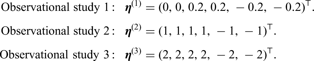
Scenario 4 considers the case where the observational data are not strictly selected, because the treatments adopted in the observational studies are not identical and ${\theta }_k$ ’s are different from each other as well as deviating from the RCT treatment effect $\theta =1$ . Scenario 5 mimics the situation where the drugs investigated in the observational studies may not even be related to the one in the RCT because treatment effects are substantially off the target. Finally, we fix the coefficient vectors ${\eta }^{(k)}$ ’s for the propensity scores for each observational study as follows:

$$\begin{array}{rl}\mathrm{Observational}\mathrm{study}1:{\mathit{\eta }}^{(1)}& =(0,0,0.2,0.2,-0.2,-0.2{)}^{\mathrm{\top }}.\\ \mathrm{Observational}\mathrm{study}2:{\mathit{\eta }}^{(2)}& =(1,1,1,1,-1,-1{)}^{\mathrm{\top }}.\\ \mathrm{Observational}\mathrm{study}3:{\mathit{\eta }}^{(3)}& =(2,2,2,2,-2,-2{)}^{\mathrm{\top }}.\end{array}$$

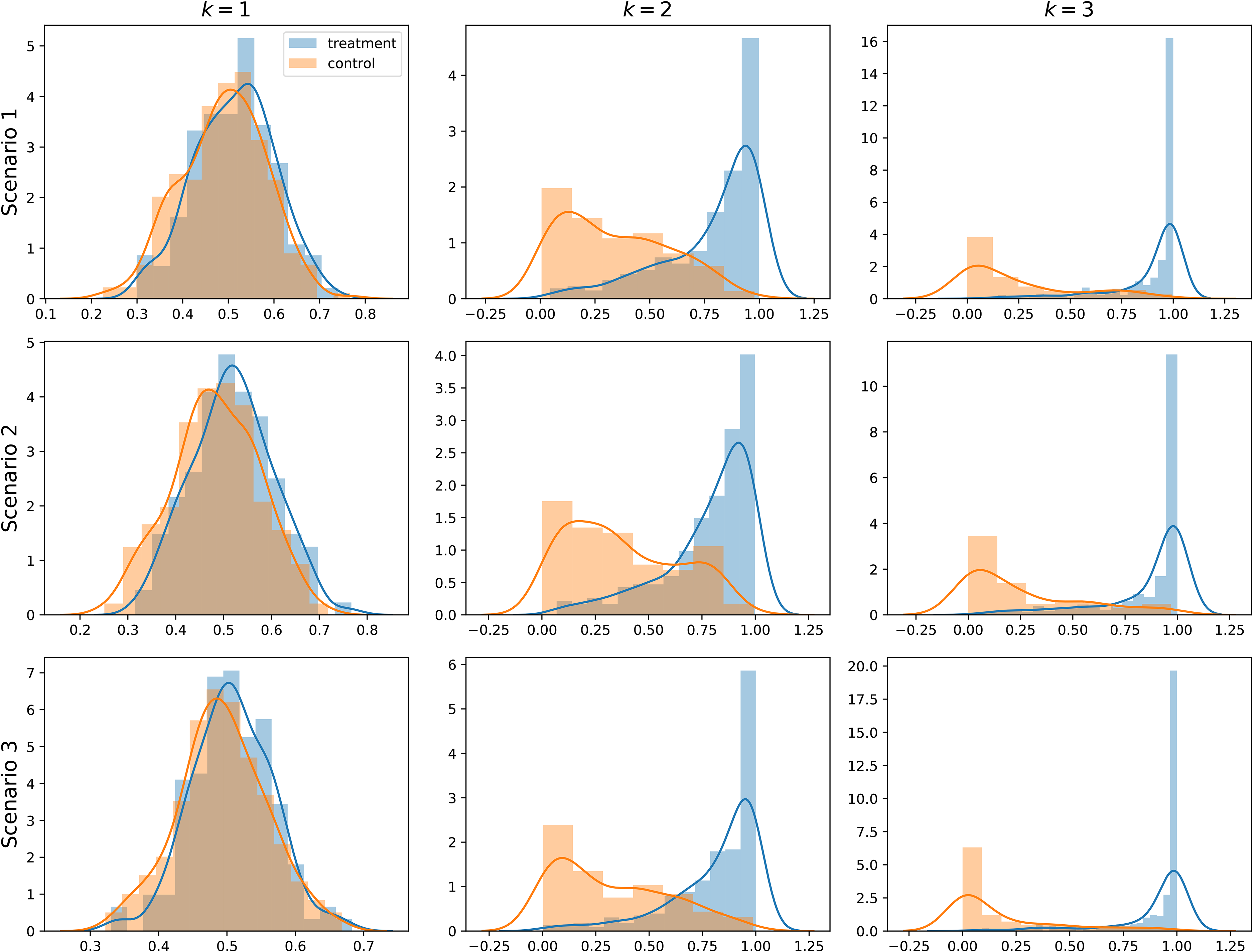
Figure 1 shows the distributions of propensity scores for three observational datasets under different generation scenarios. A wider distributional gap or separation between the treatment and control groups indicates a stronger confounding effect, which means the covariates in the corresponding dataset are more difficult to balance.

Figure 1.

Distributions of propensity scores under different scenarios for each observational dataset.

3.5 Aggregate data generation

Through the above data generation procedure, we can obtain the patient-level datasets ${\mathcal{D}}_k$ for $k=1,2,3$ . We then obtain the aggregate data ${\mathcal{S}}_k$ summarized from ${\mathcal{D}}_k$ by (i) fitting a logistic model to estimate the propensity scores; (ii) using the nearest neighbor matching (Match) ²³ or inverse probability weighting (IPW) ²⁴ to balance the observational data; and (iii) conducting inference over the balanced dataset. In the second step, we implement Match and IPW using MatchIt ²⁹ and WeightIt ³⁰ packages, respectively. For the $k$ th aggregate data ${\mathcal{S}}_k=\{{\hat{\theta }}_k,SE({\hat{\theta }}_k),n_k\}$ , the adjusted sample size $n_k$ is the number of samples after the propensity score matching whereas we take $n_k=N_k$ for IPW. Furthermore, the MLEs ${\hat{\theta }}_k$ ’s for different types of outcomes are accordingly obtained using the functions lm(), glm() and coxph() in the R language. ³¹ Finally, we adopt the robust sandwich standard error to calculate $SE({\hat{\theta }}_k)$ following the instructions in MatchIt and WeightIt.

3.6 Bayesian inference

After collecting the RCT data and aggregrating information from observational data, we conduct the Bayesian inference using the models in Section 2.1. Bayesian linear regression and logistic regression models are fitted to the continuous and binary outcomes, respectively. As for the survival outcome, we use the piecewise exponential proportional hazards model, where the baseline hazard function $h_0(t)$ is modeled as the piecewise constant function with the partition points of the time axis as $0<{\tau }_1<\dots <{\tau }_J$ . We set the number of intervals to be $J=10$ , and $\{{\tau }_1,\dots ,{\tau }_J\}$ are chosen based on the corresponding $100(j/J)$ quantiles ( $j=1,\dots ,J$ ) of observed event times. Within each interval $({\tau }_{j-1},{\tau }_j]$ , we assume a constant hazard ${\lambda }_j$ , which is assigned an NIP $\text{Gamma}(0.01,0.01)$ . Under the linear model, the priors for ${\beta }_0$ , $\beta$ , and ${\sigma }_{\epsilon }^2$ are set to be ${\beta }_0\sim N(0,{100}^2)$ , $\beta \sim N(0,{100}^2\times {\mathbf{I}}_d)$ , and ${\sigma }_{\epsilon }^2\sim \text{Inv-Gamma}(0.01,0.01)$ , and we adopt the same priors for the corresponding parameters in the logistic and Cox models. For the prior treatment effect parameter $\theta$ , we compare UIP with the NIP, which is simply defined as $\theta \sim N(0,{100}^2)$ .

All Bayesian models are implemented by PyMC3, ³² and 5,000 posterior samples are drawn for inference using the Markov chain Monte Carlo with 1,000 burn-in iterations. We simulate 200 repetitions for each configuration of data generation. Based on the repetitions, we evaluate UIP and NIP in terms of the empirical bias, root mean squared error (RMSE), and the width and coverage of the $95\text{\%}$ credible interval (CrI) for the parameter $\theta$ . The $95\text{\%}$ CrI is constructed based on $2.5\text{\%}$ and $97.5\text{\%}$ quantiles from the posterior samples.

3.7 Results

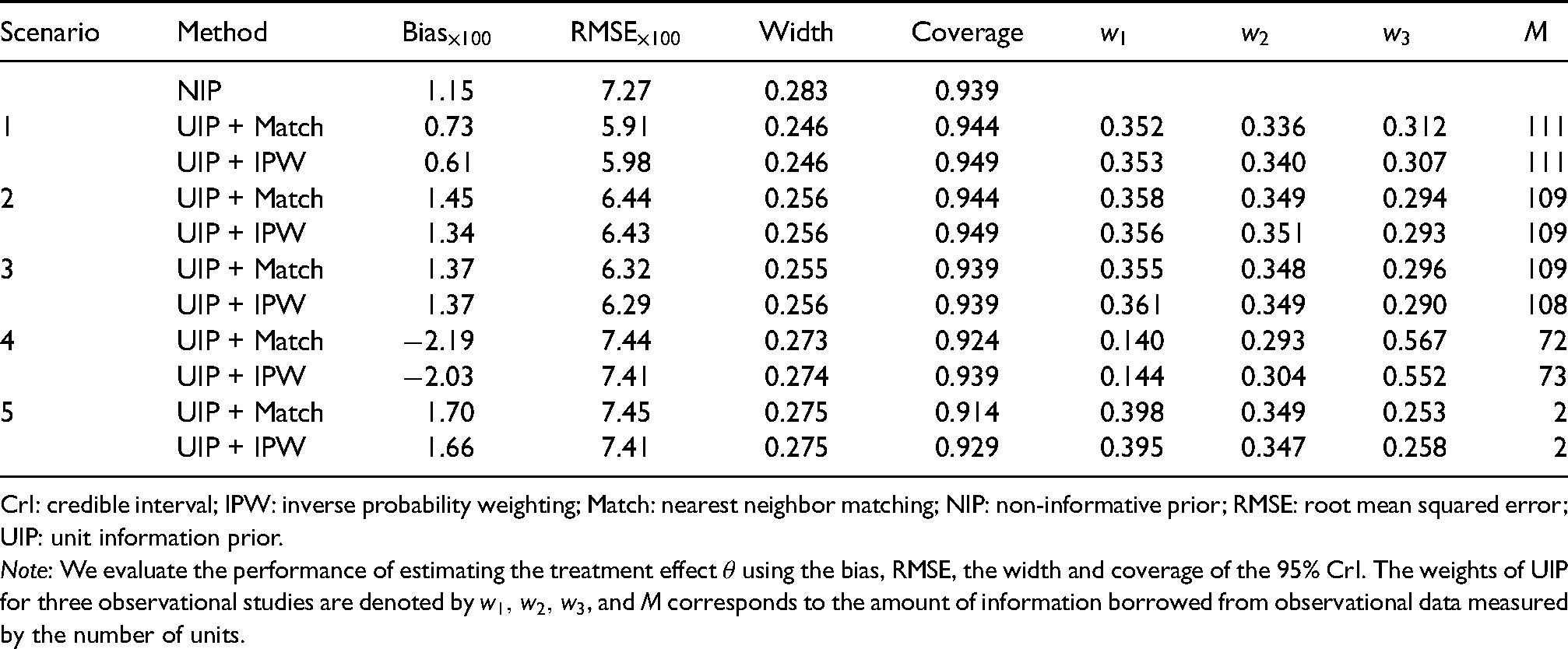
Table 1 presents the simulation results for the continuous outcome. Because NIP does not require observational data, its results are the same across different scenarios. Considering the UIP, we observe that it can effectively improve the precision of estimating $\theta$ in terms of RMSE under various scenarios and both balancing approaches. In addition, UIP reduces the bias under Scenario 1 when the observational data share the same treatment effect with RCT, and only incurs a minor increase in bias under Scenarios 2 and 3 when there exist heterogeneous treatment effects and covariates between the RCT and observational studies. For the CrI, UIP yields shorter widths and slightly larger values of coverage probability compared with NIP for the first three scenarios, which is due to the precise estimation of the treatment effect after synthesizing the observational evidence. Furthermore, UIP tends to borrow more information from ${\mathcal{D}}_1$ and ${\mathcal{D}}_2$ as demonstrated by larger values of $w_1$ and $w_2$ in Scenarios 2 and 3. It is due to the empirical fact that the first two datasets can more accurately estimate ${\theta }_1$ and ${\theta }_2$ , which are closer to $\theta$ of the RCT, after balancing the relative less confounded covariates (e.g. $n_1=482$ , $n_2=369$ , and $n_3=366$ under Scenario 3). The values of $w_k$ ’s are more distinctive when the deviations of ${\theta }_k$ ’s from $\theta$ vary substantially under Scenario 4. The total amount of borrowed information $M$ is slightly above half of the RCT sample size $(n=200)$ for the UIP approaches when ${\theta }_k$ ’s are close to $\theta$ under Scenarios 1 to 3. A drastic decrease can be observed for $M$ under Scenarios 4 and 5, where the treatment effects in the observational studies are more extreme relative to $\theta$ in the RCT. In Scenario 5, almost no information is borrowed from observational studies due to such a small value of $M=2$ , and thus UIP delivers performance close to NIP in terms of all evaluation metrics.

Table 1.

The simulation results of different prior methods for continuous outcomes (linear regression) under three scenarios.

Scenario	Method	${\text{{Bias}}}_{\times 100}$	${\text{{RMSE}}}_{\times 100}$	Width	Coverage	$w_1$	$w_2$	$w_3$	$M$
	NIP	1.15	7.27	0.283	0.939
1	UIP + Match	0.73	5.91	0.246	0.944	0.352	0.336	0.312	111
	UIP + IPW	0.61	5.98	0.246	0.949	0.353	0.340	0.307	111
2	UIP + Match	1.45	6.44	0.256	0.944	0.358	0.349	0.294	109
	UIP + IPW	1.34	6.43	0.256	0.949	0.356	0.351	0.293	109
3	UIP + Match	1.37	6.32	0.255	0.939	0.355	0.348	0.296	109
	UIP + IPW	1.37	6.29	0.256	0.939	0.361	0.349	0.290	108
4	UIP + Match	$-$ 2.19	7.44	0.273	0.924	0.140	0.293	0.567	72
	UIP + IPW	$-$ 2.03	7.41	0.274	0.939	0.144	0.304	0.552	73
5	UIP + Match	1.70	7.45	0.275	0.914	0.398	0.349	0.253	2
	UIP + IPW	1.66	7.41	0.275	0.929	0.395	0.347	0.258	2

CrI: credible interval; IPW: inverse probability weighting; Match: nearest neighbor matching; NIP: non-informative prior; RMSE: root mean squared error; UIP: unit information prior. Note: We evaluate the performance of estimating the treatment effect $\theta$ using the bias, RMSE, the width and coverage of the 95% CrI. The weights of UIP for three observational studies are denoted by $w_1,w_2,w_3$ , and $M$ corresponds to the amount of information borrowed from observational data measured by the number of units.

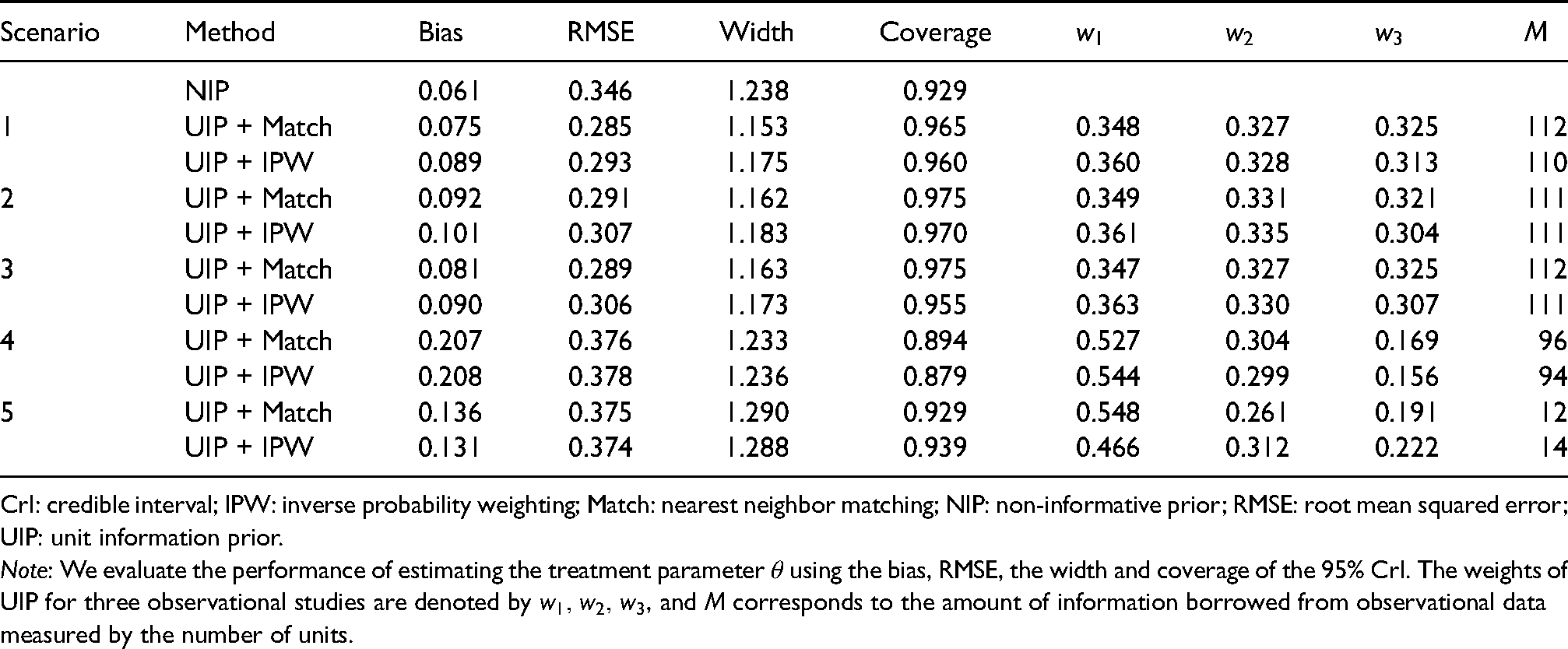
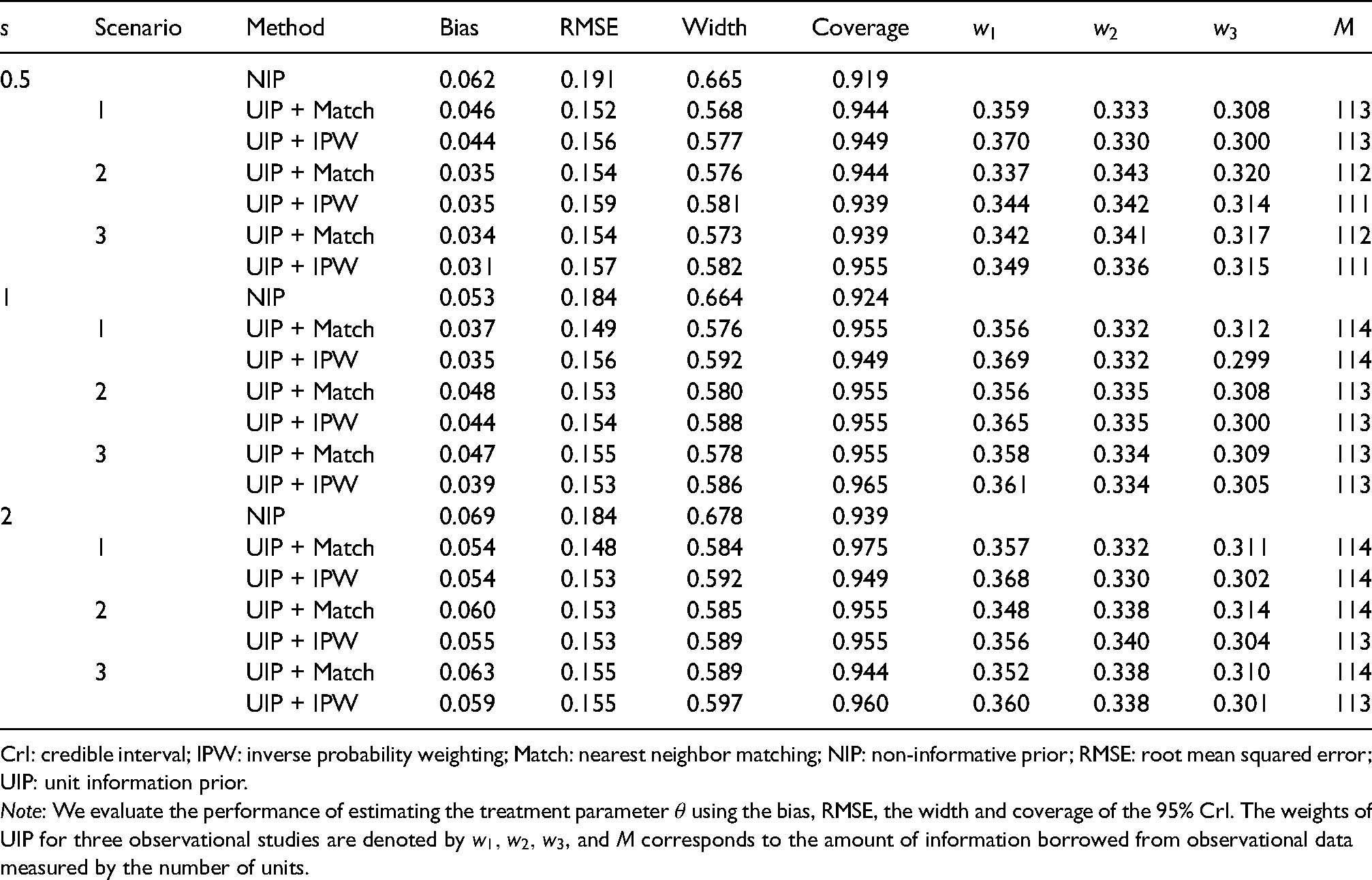
The results for the binary outcome are shown in Table 2. Clearly, the UIP can reduce the RMSE under Scenarios 1 to 3, in contrast, to NIP with a minor sacrifice in bias. Narrower CrIs can be obtained under UIP with coverage probabilities closer to the nominal level. Under Scenarios 4 and 5, the first two datasets contribute more to the current RCT as evidenced by relatively larger values of $w_1$ and $w_2$ in comparison with $w_3$ . The UIP borrows much less information in Scenario 5 as indicated by small values of $M$ , because of substantial differences between the treatment effects of the observational studies and RCT. The UIP also improves the inference of $\theta$ for the survival outcome as shown by Table 3. The UIP can reduce both the bias and RMSE compared with NIP for decreasing ( $s=0.5$ ), constant ( $s=1$ ), and increasing ( $s=2$ ) baseline hazards, which shows the robustness of UIP with respect to different types of hazard functions. It also yields tighter CrIs for $\theta$ with coverage probabilities closer to the nominal level. In summary, UIP can enhance the inference of the RCT via integrating real-world evidence, and the improvement is more evident when the RCT and observational studies are similar.

Table 2.

The simulation results of different prior methods for binary outcomes (logistic regression) under three scenarios.

Scenario	Method	Bias	RMSE	Width	Coverage	$w_1$	$w_2$	$w_3$	$M$
	NIP	0.061	0.346	1.238	0.929
1	UIP + Match	0.075	0.285	1.153	0.965	0.348	0.327	0.325	112
	UIP + IPW	0.089	0.293	1.175	0.960	0.360	0.328	0.313	110
2	UIP + Match	0.092	0.291	1.162	0.975	0.349	0.331	0.321	111
	UIP + IPW	0.101	0.307	1.183	0.970	0.361	0.335	0.304	111
3	UIP + Match	0.081	0.289	1.163	0.975	0.347	0.327	0.325	112
	UIP + IPW	0.090	0.306	1.173	0.955	0.363	0.330	0.307	111
4	UIP + Match	0.207	0.376	1.233	0.894	0.527	0.304	0.169	96
	UIP + IPW	0.208	0.378	1.236	0.879	0.544	0.299	0.156	94
5	UIP + Match	0.136	0.375	1.290	0.929	0.548	0.261	0.191	12
	UIP + IPW	0.131	0.374	1.288	0.939	0.466	0.312	0.222	14

CrI: credible interval; IPW: inverse probability weighting; Match: nearest neighbor matching; NIP: non-informative prior; RMSE: root mean squared error; UIP: unit information prior. Note: We evaluate the performance of estimating the treatment parameter $\theta$ using the bias, RMSE, the width and coverage of the 95% CrI. The weights of UIP for three observational studies are denoted by $w_1,w_2,w_3$ , and $M$ corresponds to the amount of information borrowed from observational data measured by the number of units.

Table 3.

The simulation results of different prior methods for survival outcomes (Cox regression) under various cases, where $s$ determines the shape of the baseline hazard function.

$s$	Scenario	Method	Bias	RMSE	Width	Coverage	$w_1$	$w_2$	$w_3$	$M$
0.5		NIP	0.062	0.191	0.665	0.919
	1	UIP + Match	0.046	0.152	0.568	0.944	0.359	0.333	0.308	113
		UIP + IPW	0.044	0.156	0.577	0.949	0.370	0.330	0.300	113
	2	UIP + Match	0.035	0.154	0.576	0.944	0.337	0.343	0.320	112
		UIP + IPW	0.035	0.159	0.581	0.939	0.344	0.342	0.314	111
	3	UIP + Match	0.034	0.154	0.573	0.939	0.342	0.341	0.317	112
		UIP + IPW	0.031	0.157	0.582	0.955	0.349	0.336	0.315	111
1		NIP	0.053	0.184	0.664	0.924
	1	UIP + Match	0.037	0.149	0.576	0.955	0.356	0.332	0.312	114
		UIP + IPW	0.035	0.156	0.592	0.949	0.369	0.332	0.299	114
	2	UIP + Match	0.048	0.153	0.580	0.955	0.356	0.335	0.308	113
		UIP + IPW	0.044	0.154	0.588	0.955	0.365	0.335	0.300	113
	3	UIP + Match	0.047	0.155	0.578	0.955	0.358	0.334	0.309	113
		UIP + IPW	0.039	0.153	0.586	0.965	0.361	0.334	0.305	113
2		NIP	0.069	0.184	0.678	0.939
	1	UIP + Match	0.054	0.148	0.584	0.975	0.357	0.332	0.311	114
		UIP + IPW	0.054	0.153	0.592	0.949	0.368	0.330	0.302	114
	2	UIP + Match	0.060	0.153	0.585	0.955	0.348	0.338	0.314	114
		UIP + IPW	0.055	0.153	0.589	0.955	0.356	0.340	0.304	113
	3	UIP + Match	0.063	0.155	0.589	0.944	0.352	0.338	0.310	114
		UIP + IPW	0.059	0.155	0.597	0.960	0.360	0.338	0.301	113

CrI: credible interval; IPW: inverse probability weighting; Match: nearest neighbor matching; NIP: non-informative prior; RMSE: root mean squared error; UIP: unit information prior. Note: We evaluate the performance of estimating the treatment parameter $\theta$ using the bias, RMSE, the width and coverage of the 95% CrI. The weights of UIP for three observational studies are denoted by $w_1,w_2,w_3$ , and $M$ corresponds to the amount of information borrowed from observational data measured by the number of units.

Based on Tables 1 to 3, we can also gain some insight into the factors that affect $w_k$ ’s and $M$ . In general, the weights are determined by both treatment effects and the covariate confounding effects in the observational data relative to the RCT, and the impact of the treatment effect is more evident. In Scenario 1, all observational data share the same treatment effect with the RCT, that is, ${\theta }_1={\theta }_2={\theta }_3=\theta$ , but they have different degrees of covariate confounding effect. Since a greater confounding effect would lead to a larger standard error or a more biased treatment effect estimator, the first two datasets, ${\mathcal{D}}_1$ and ${\mathcal{D}}_2$ , tend to be more informative and we thus observe $w_1>w_2>w_3$ . In Scenario 2, although ${\theta }_2$ is closer to $\theta$ than ${\theta }_1$ , we observe $w_2<w_1$ in most cases, because the covariate confounding effect has a greater impact on the weights than the treatment effects when all ${\theta }_k$ ’s are close to $\theta$ . Scenarios 4 and 5 show that the observational treatment effects are more influential than the confounding effect when ${\theta }_k$ ’s deviate far from $\theta$ . Furthermore, by comparing Scenario 2 and Scenario 3, the patient population does not have a strong influence on the order of $w_k$ ’s.

The parameter $M$ is affected by the level of consistency between the observational studies and the current RCT, ²² for which the more inconsistency the smaller value of $M$ . Scenarios 1 to 3 show that the patient population does not impose a strong influence on the values of $M$ . Scenarios 4 and 5 show that $M$ is sensitive to the dissimilarity between ${\theta }_k$ ’s and $\theta$ .

4 Real application

In the COVID-19 pandemic era, numerous studies have been conducted to find effective treatments. We illustrate the application of UIP by re-analyzing a randomized trial, ³³ which was launched to evaluate the efficacy of hydroxychloroquine (HCQ) in reducing the in-hospital mortality of COVID-19 compared with the placebo. The parameter of interest is the HR between the HCQ and placebo groups. Due to inaccessibility to the original survival data, we use the R package IPDfromKM^34,35 to reconstruct the patient-level data from the Kaplan–Meier curves of the HCQ and placebo groups in Figure 2 of the original paper. ³³ The reconstructed dataset contains 208 samples with 104 samples from the HCQ group and 104 from the control group. We obtain the outcome variable $Y_i$ , treatment indicator $Z_i$ , and the event indicator ${\delta }_i$ for the $i$ th reconstructed observation.

Based on the reconstructed data, we re-estimate the HR of receiving HCQ, respectively, using NIP and UIP under the piecewise exponential model without covariates, i.e.that is, $\beta =0$ . In addition to the Bayesian approaches, we also adopt the frequentist Cox proportional hazards model via the R function coxph() to estimate the HR. For the UIP, we collect the aggregate information from four different observational studies denoted by their respective published journals: PLoS One (PLoS), ³⁶ New England Journal of Medicine (NEJM), ²⁷ American Journal of Epidemiology (AJE), ³⁷ and Clinical Infectious Diseases (CID). ³⁸ The four observational studies are selected following the criteria detailed in Section 2.2 with the aforementioned RCT as the template. First, those studies all considered the effect of HCQ therapy in reducing the mortality of COVID-19 and used the HR to measure the treatment efficacy. Second, similar to the RCT, the enrolled samples in those studies were all non-pregnant hospitalized patients who had been diagnosed with COVID-19 and did not participate in other trials, and the majority of them were middle-aged or older people. Finally, those studies all fitted the Cox proportional hazards model with the propensity score adjustment to estimate the HR, where the propensity score weighting was used for NEJM, AJE, and CID, while PLoS leveraged the propensity score stratification. The summary information provided in the published papers includes sample size, the estimated HR $\exp ({\hat{\theta }}_k)$ , and its $95\text{\%}$ CI. We perform the logarithmic transformation to obtain ${\mathcal{S}}_k=\{{\hat{\theta }}_k,\text{SE}({\hat{\theta }}_k),n_k\}$ , $k=1,\dots ,4$ . The UIP and NIP are then, respectively, applied to the Bayesian model following the same configurations used in the simulation.

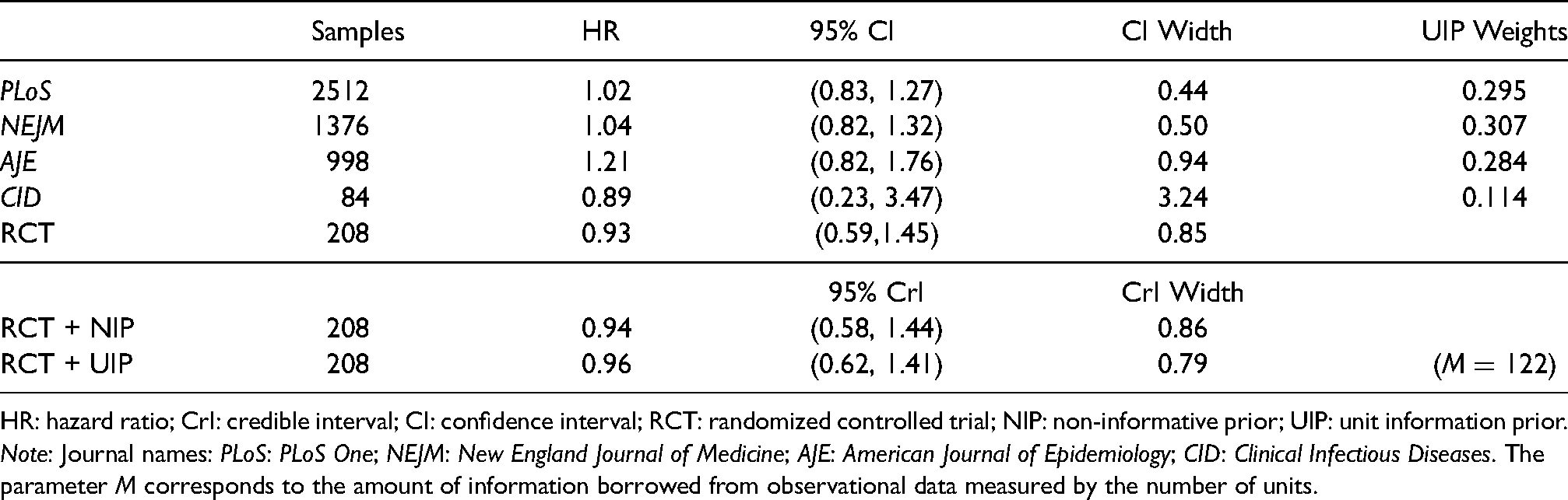
We report the estimated HR for the reconstructed RCT data and the summary information of the historical studies in Table 4. The estimated HR under UIP is 0.96 (95% CrI, 0.62–1.41), which has a narrower CrI than that under NIP, 0.94 (95% CrI, 0.58–1.44), and the frequentist counterpart, 0.93 (95% CI, 0.59–1.45), thus demonstrating the effectiveness of historical information borrowing. The parameter $M$ is estimated to be 122 for UIP, indicating that UIP synthesizes an intermediate amount of observational information in contrast with the sample size of the randomized trial. The UIP weights for (PLoS, NEJM, AJE, CID) are $(w_1,\dots ,w_4)=(0.295,0.307,0.284,0.114)$ , suggesting that the least amount of information is borrowed from CID and more information is incorporated from NEJM and PLoS. The sample sizes of the two studies in NEJM and PLoS are both large and their estimated HRs have narrower CIs and, as a result, UIP tends to borrow more evidence from more reliable studies. In summary, the re-analyzed HR based on UIP concludes that there is no significant improvement in the post-hospitalization mortality caused by COVID-19 for patients receiving HCQ, which is consistent with the claim in the original article but the evidence via incorporating the four observational studies is clearly more convincing.

Table 4.

The estimated HR with the CI/CrI for the reconstructed RCT and four historical observational studies using their respective journal names.

	Samples	HR	95% CI	CI Width	UIP Weights
PLoS	2512	1.02	(0.83, 1.27)	0.44	0.295
NEJM	1376	1.04	(0.82, 1.32)	0.50	0.307
AJE	998	1.21	(0.82, 1.76)	0.94	0.284
CID	84	0.89	(0.23, 3.47)	3.24	0.114
RCT	208	0.93	(0.59,1.45)	0.85
			95% CrI	CrI Width
RCT + NIP	208	0.94	(0.58, 1.44)	0.86
RCT + UIP	208	0.96	(0.62, 1.41)	0.79	( $M=122$ )

HR: hazard ratio; CrI: credible interval; CI: confidence interval; RCT: randomized controlled trial; NIP: non-informative prior; UIP: unit information prior. Note: Journal names: PLoS: PLoS One; NEJM: New England Journal of Medicine; AJE: American Journal of Epidemiology; CID: Clinical Infectious Diseases. The parameter $M$ corresponds to the amount of information borrowed from observational data measured by the number of units.

5 Discussion

For a more comprehensive analysis of a current RCT, we develop the UIP methodology for synthesizing the evidence from historical observational studies into the analysis of the RCT data. The UIP is readily applicable to various common types of outcomes considered in clinical trials, and it only requires published summary information. The prior automatically quantifies the amount of information borrowed from each study and simultaneously considers the unamendable bias in the real-world evidence. Extensive numerical experiments show that the UIP can improve the statistical efficiency of inference for the RCT. There are several promising directions to further extend the idea of UIP for information borrowing. For example, it is of interest to leverage the prior to incorporate the patient-level observational data into the single-arm trials as discussed by Liu et al. ¹³ Furthermore, one can investigate how UIP affects the type I error and power, and its possible application in determining the sample size of an RCT at the design stage. The UIP also sheds light on a meta-analysis from the information borrowing aspect, which warrants further investigation. Finally, one may consider the synthesis when individual patient-level data are available for both the RCT and observational studies, for which other existing methods, such as the power prior or commensurate prior, can also be applicable. The codes for the numerical studies are available at https://github.com/BobZhangHT/UIP4RCT.