Sage Journals: Discover world-class research

Abstract

Meta-analytic methods may be used to combine evidence from different sources of information. Quite commonly, the normal–normal hierarchical model (NNHM) including a random-effect to account for between-study heterogeneity is utilized for such analyses. The same modeling framework may also be used to not only derive a combined estimate, but also to borrow strength for a particular study from another by deriving a shrinkage estimate. For instance, a small-scale randomized controlled trial could be supported by a non-randomized study, e.g. a clinical registry. This would be particularly attractive in the context of rare diseases. We demonstrate that a meta-analysis still makes sense in this extreme case, effectively based on a synthesis of only two studies, as illustrated using a recent trial and a clinical registry in Creutzfeld-Jakob disease. Derivation of a shrinkage estimate within a Bayesian random-effects meta-analysis may substantially improve a given estimate even based on only a single additional estimate while accounting for potential effect heterogeneity between the studies. Alternatively, inference may equivalently be motivated via a model specification that does not require a common overall mean parameter but considers the treatment effect in one study, and the difference in effects between the studies. The proposed approach is quite generally applicable to combine different types of evidence originating, e.g. from meta-analyses or individual studies. An application of this more general setup is provided in immunosuppression following liver transplantation in children.

Keywords

Random-effects meta-analysis Bayesian statistics between-study heterogeneity shrinkage estimation

1 Introduction

In clinical research of orphan diseases, one of the major problems is often the recruitment of a sufficient number of subjects to perform a meaningful clinical trial. Examples include neuromyelitis optica,¹ myocarditis,² and Creutzfeld-Jakob disease (CJD).³ In such cases, it may be possible to gain some power by using more sophisticated trial designs, and it is often desirable to be able to formally utilize additional information external to the actual trial, which may be implemented via the use of informative prior distributions in the eventual analysis.⁴ The external information could be in the form of related studies or elicited expert opinion.⁵ For instance, in the context of a small-scale randomized controlled trial in idiopathic nephrotic syndrome in children, a rare condition, Thall et al.⁶ recently proposed the elicitation of expert opinions on response probabilities based on the bins-and-chips approach.⁷

When considering external evidence, the obvious danger is that a too simplistic approach may lead to a “naïve” pooling of initially separate data. For example, while data from non-randomized studies (e.g. clinical registries) may undoubtedly contribute complementing information to a randomized clinical trial, one may want to prevent a complete mixing of both types of data, which would in a sense also invalidate the original randomization. Rather it seems desirable to stratify the analysis for the different sources by explicitly allowing for potential heterogeneity between data sets, which then implicitly downweights the impact on one another. Here the weights depend on the observed similarity of estimates, also known as dynamic borrowing of information.⁸ The eventual analysis then may refer explicitly to the outcome of the randomized trial, and not to some overall average, as generally more weight is placed on evidence from randomized controlled trials.

A simple approach originally proposed by Pocock⁹ was recently implemented by Schoenfeld et al.,¹⁰ who investigated the use of adult data to support the analysis of a paediatric trial, and who utilized a variance component of known (elicited) magnitude to account for heterogeneity between the two studies' estimates. A closely related approach is implemented in the normal-normal hierarchical model (NNHM) that is commonly utilized in random-effects meta-analysis; the difference essentially is that heterogeneity is treated as an unknown for which a prior distribution may be specified. Technically, inference on the study of primary interest is done by investigating the corresponding shrinkage estimate. The contribution of information from additional studies then may readily be evaluated by considering the corresponding meta-analytic-predictive (MAP) prior.^11,12 The NNHM is readily generalized (and in fact most commonly used) for combining more than two studies; such an approach may e.g. be used to extrapolate information from early-phase studies in the approval process.¹² In the case of two studies, the NNHM can also be shown to be to some extent equivalent to a similar, more general model specification as we will explain below.

While the interpretation of parameters within the familiar NNHM context is straightforward and with the inclusion of an unknown heterogeneity parameter it is intended that evidence from separate studies is sufficiently loosely connected to provide a robust estimation framework, it is not obvious to what extent this approach actually improves estimates in the extreme case of only two studies or more generally two data sources. Here we develop a suitable statistical hierarchical model to include two sources of data, e.g. two studies or meta-analyses. Within the proposed model, we describe a shrinkage estimator and inference methods including posterior predictive p-values. Furthermore, the value of this approach in the particular case of only two studies is evaluated in simulations.

The manuscript is organized as follows. In the next section, we present the statistical model and, in particular, shrinkage estimation and inference. The following sections are dedicated to a simulation study investigating the operating characteristics of the proposed methodology and an application in CJD. Motivated by a meta-analysis investigating the effect of immunosuppression in paediatric liver transplantation patients, we extend the shrinkage applications to more general settings considering two data sources, e.g. two meta-analyses, rather than two studies. Finally, we close with some conclusions and a brief discussion.

2 Statistical model and shrinkage estimation

2.1 The normal–normal hierarchical model

The most commonly used model for random-effects meta-analysis is the normal-normal hierarchical model (NNHM). This model is applicable for the joint analysis of several (k) real-valued effect measurements y_i that have individual standard errors σ_i associated ( $i = 1, \dots, k$ ). Here it is assumed that each observation y_i is a noisy measurement of an underlying true value θ_i with a normally distributed offset whose magnitude is given through the (known) standard error σ_i

y_{i} | θ_{i} \sim N (θ_{i}, σ_{i}^{2})

(1)

The θ_i then may be more or less similar across measurements; at the study level, a certain amount of heterogeneity is anticipated by introducing another variance component τ and assuming

θ_{i} | μ, τ \sim N (μ, τ^{2})

(2)

where the overall effect μ and heterogeneity

τ \geq 0

are unknown. If τ = 0, the model simplifies to the fixed-effect model, in which

θ_{1} = \dots = θ_{k} = μ

, but in general this is a random-effects model.^13–15 In the following, we will mostly be concerned with the special case of analyzing only k = 2 studies. Note that while classically, in the meta-analysis context, the y_i usually originate from different studies, more generally these may also be estimates of other kinds, e.g. estimates from meta-analyses.

2.2 Shrinkage estimation

Quite commonly, the main interest lies in determining the overall effect μ. When the aim of the analysis is to provide a basis for planning a new study, it may also be of interest to predict a future outcome $θ_{k + 1}$ . In some cases, however, it is of interest to derive an updated estimate for a particular (ith) study effect θ_i, which is informed by the remaining studies under consideration.

If the heterogeneity τ was zero, then the model would reduce to the fixed-effect model, and all estimates y_i would effectively relate to the same parameter ( $θ_{i} = μ$ ), which may then be jointly estimated by simply averaging the estimates y_i (with “inverse variance” weights). If the heterogeneity appears to be close to zero, then the model will behave similarly to the fixed-effect model, and all estimated study effects θ_i will be “shrunk” towards the estimated overall mean μ to some degree. If on the other hand the heterogeneity is large, then there is very little to be learned from one estimate (y_i) about another parameter (θ_j, $j \neq i$ ), and different estimates only provide very little support to one another. Effectively, this results in more or less shrinkage towards the overall mean μ, depending on the apparent heterogeneity in the data.^12,16 This shrinkage estimation of study-specific means θ_i, which is also known as best linear unbiased prediction (BLUP) in a frequentist framework,^17–19 will be our focus in the following. When the heterogeneity τ is assumed fixed and known (and an improper uniform prior for μ is used), then the frequentist and Bayesian approaches lead to identical mean effect (μ)²⁰ as well as shrinkage estimates (θ_i)^17,21; in general, however, these are different.

2.3 The Bayesian approach to meta-analysis

The inference problems within the NNHM may be approached using frequentist or Bayesian methods.^{13–15,21,22} A Bayesian approach has proven especially useful in cases where large-sample asymptotics do not apply,²³ e.g. for the analysis of few studies²⁰ or even only two studies.²⁴ Here, we will follow a Bayesian approach and investigate its properties in some more detail.

Within the NNHM we have several unknowns; first the study-specific effects θ_i, whose hyperprior is given through Equation (2). For the overall mean effect μ, it is often convenient to use a non-informative (improper) uniform prior. The heterogeneity $τ \geq 0$ determines the expected variability between individual studies; depending on the measurement scale of the considered effects, in practical applications a plausible upper bound can usually be specified. Half-normal (HN) priors (e.g. with scale parameters 0.5 or 1.0) have proven useful, for example, in the context of logarithmic odds-ratio (log-OR) endpoints.^20,22,25 An analogous reasoning similarly applies for many log-transformed endpoints, like relative risks or hazard ratios; if different studies are considered unlikely to differ by more than a certain factor, then one can usually translate this into a prior specification for the heterogeneity τ on the logarithmic scale.^21,22

The heterogeneity τ is usually considered a nuisance parameter, while the primary interest is in inferring the overall effect (μ), a prediction ( $θ_{k + 1}$ ), or a shrinkage estimate (θ_i). Within the Bayesian framework, shrinkage estimation may be motivated in two different ways; the meta-analytic-combined (MAC) approach simply considers the shrinkage estimate as one of the parameters in the NNHM model, where all k studies are analyzed jointly. The meta-analytic-predictive (MAP) approach on the other hand considers the same problem sequentially: first, all but the ith study are analyzed, and the derived posterior (predictive) distribution then constitutes the prior for the analysis of the ith study. Both approaches can be shown to be equivalent and lead to identical results,¹¹ but the MAP approach allows to explicate the information ‘borrowed’ from the additional estimates via the MAP prior. Technically, inference requires integration over the parameters’ posterior distribution,^16,22 for example, to derive the relevant marginal posterior distribution for shrinkage estimation ( $p (θ_{i} | y_{1}, y_{2}, σ_{1}, σ_{2})$ ). Computations for inference within the NNHM may be performed in R using the bayesmeta package.^21,26 In the following, the shown estimates will be posterior medians, and credible intervals are determined as shortest posterior intervals.

2.4 Posterior predictive p-values

Posterior predictive p-values are conceptually closely related to “classical” p-values, and were originally developed in the context of model checking.^16,27,28 The definition is relatively straightforward; like a classical p-value, it is based on a null hypothesis H₀ and a pre-specified (“test-”) statistic or “discrepancy variable” $T (\cdot)$ , which is a function of the data. The statistic T is (as usual) defined so that it is sensitive to deviations from the null hypothesis. The realised statistic value T(y) then is determined for the present data set y. In order to judge whether the statistic value is “sufficiently extreme” to constitute evidence against the null hypothesis, it is compared against its posterior predictive distribution, conditional on H₀.

Similarly to the usual p-values, this means a comparison against values of the statistic amongst data sets that might have occurred conditioning on the observed data as well as the null hypothesis. Technically, posterior predictive p-values are often easily computed using Monte Carlo sampling, which here means first drawing parameter values from the intersection of the parameters' posterior distribution and null hypothesis, then drawing a data set $y^{⋆}$ from the corresponding predictive distribution, and determining the statistic value $T (y^{⋆})$ . Repeated sampling then allows to explore the relevant distribution of statistic values and eventually compute p-values via the corresponding tail probabilities. While posterior predictive p-values generally do not follow a uniform distribution under the null hypothesis, the deviation is usually on the conservative side.^27,29

The test statistic to be used needs to be pre-specified. For instance, an obvious choice for the overall effect μ may be the posterior probability of a non-beneficial effect, i.e.

T (y) = P (μ > 0 | y)

(3)

The null hypothesis then is usually specified for a certain parameter as one- or two-sided. Accordingly, the test statistic's relevant distribution (or the sampling scheme, in case of MCMC computation) as well as the statistic's rejection region is affected. Computation of posterior predictive p-values is also implemented in the bayesmeta R package.²¹

2.5 The reference model as an alternative variation of the NNHM

When meta-analyzing a pair of estimates, the common NNHM may sometimes be hard to motivate, as an exchangeable model of both estimates θ_i centered around a common mean value μ may seem inappropriate. Consider for example the joint analysis of randomized and observational data; reference to a common mean parameter μ or identical variances $τ^{2}$ may be counterintuitive in such a case. An “asymmetric” treatment of both estimates in terms of a “reference” estimate and a “secondary”, related observable with an uncertain amount of offset associated may seem more appealing. It is possible to formulate a slight variation of the NNHM following this second approach, which may seem more realistic, and for which one can then show that both approaches are equivalent as far as shrinkage estimates are concerned. In the following, we will refer to this model variation as the reference model.

Suppose that the prior for the effect μ in the NNHM is given by an (improper) uniform distribution, and that the heterogeneity prior is defined through a density $p_{⋆} (τ)$ . Then the model variation is defined as follows; for the observables y_i we assume

y_{i} | ϑ_{i} \sim N (ϑ_{i}, σ_{i}^{2})

(4)

which so far is analogous to the NNHM setup. At the next hierarchy level, we then specify

ϑ_{1} | α, β \sim N (α, 0) (i . e ., ϑ_{1} = α),

(5)

ϑ_{2} | α, β \sim N (α, β^{2})

(6)

where the “effect” parameter α again has an improper uniform prior and the variance component β now has a prior density given by

\frac{1}{\sqrt{2}} p_{⋆} (\frac{β}{\sqrt{2}})

. The parameter β hence has a prior that is scaled by a factor of

\sqrt{2}

relative to τ, which corresponds to a factor 2 difference for the squared parameters (the variances).

The reference model parametrisation of the problem is different here in that the two observables y_i are treated asymmetrically. The first one (y₁) measures the parameter α (the reference) “directly”, while the second one (y₂) includes an additional offset with variance $β^{2}$ . The variance component β again implements the heterogeneity between the first and second observable, but in a slightly different manner than in the original NNHM. While the parameterizations are different, the associated shrinkage estimates (for θ_i or $ϑ_{i}$ ) are identical, as shown in detail in Appendix 1. Since $ϑ_{1} = α$ , the shrinkage estimate for $ϑ_{1}$ is identical to an estimate of α in this context. The NNHM's heterogeneity (τ) prior needs to be re-scaled by a factor of $\sqrt{2}$ to yield the corresponding β prior. Note, however, that the equivalence only holds for the case of k = 2 estimates, and an (improper) uniform effect prior; for other cases, the model would need to be adapted accordingly.

As has been pointed out by Neuenschwander et al.,³⁰ the model may also be regarded as a special case of Pocock's bias model, or the model underlying the commensurate prior. In both instances, for the case of k = 2 studies, the discrepancy between the two underlying parameters (here: $ϑ_{1}$ and $ϑ_{2}$ ) is also modeled via a variance parameter analogous to $β^{2}$ above. The connection is made somewhat differently in the power prior model,³¹ where the external data are downweighted via an exponential parameter between 0 and 1 that is applied to part of the likelihood function. For a given τ (or β) value, the approaches are again identical when the exponential parameter is set to be $(2 \frac{τ^{2}}{σ_{2}^{2}} + 1) - 1$ or $(\frac{β^{2}}{σ_{2}^{2}} + 1)^{- 1}$ .

3 Dependency of the shrinkage estimate on the observed heterogeneity

In the following, we investigate the effect of varying the input data on the resulting shrinkage estimates. The setup is similar to the one also adopted in the subsequent simulation study; we consider the case of two estimates (y₁ and y₂) with standard errors $σ_{1} = 0.8$ and $σ_{2} = 0.2$ , and we assume a uniform prior for μ and a half-normal (HN) prior with scale 0.5 for the heterogeneity τ. We set $y_{1} = 0$ and then vary the difference between the estimates ( $y_{2} - y_{1}$ ), which is in a sense also the “observed heterogeneity” in the data. Then we derive the shrinkage estimate for the first parameter θ₁.

Figure 1 (top panel) illustrates the effect on the shrinkage estimate and the corresponding 95% credible interval. One can see how the estimate (posterior median of θ₁) moves (mostly) in concordance with the second estimate (y₂) and that the resulting interval is narrowest when y₁ and y₂ are in close agreement. For larger differences, the estimated heterogeneity increases, less borrowing of information takes place, the interval widens and the estimate of θ₁ is less attracted towards y₂. Eventually the shrinkage interval exhibits a certain degree of robustness and barely changes with increasing difference. This robustness feature may be explained by the fact that implicitly the meta-analysis is equivalent to an analysis of the first study using the MAP-prior based on the second study.¹¹ The prior derived via the hierarchical model from the first study then is rather vague and heavy-tailed, leading to the robust behaviour.³²

Figure 1.

Effect of varying the difference between quoted estimates (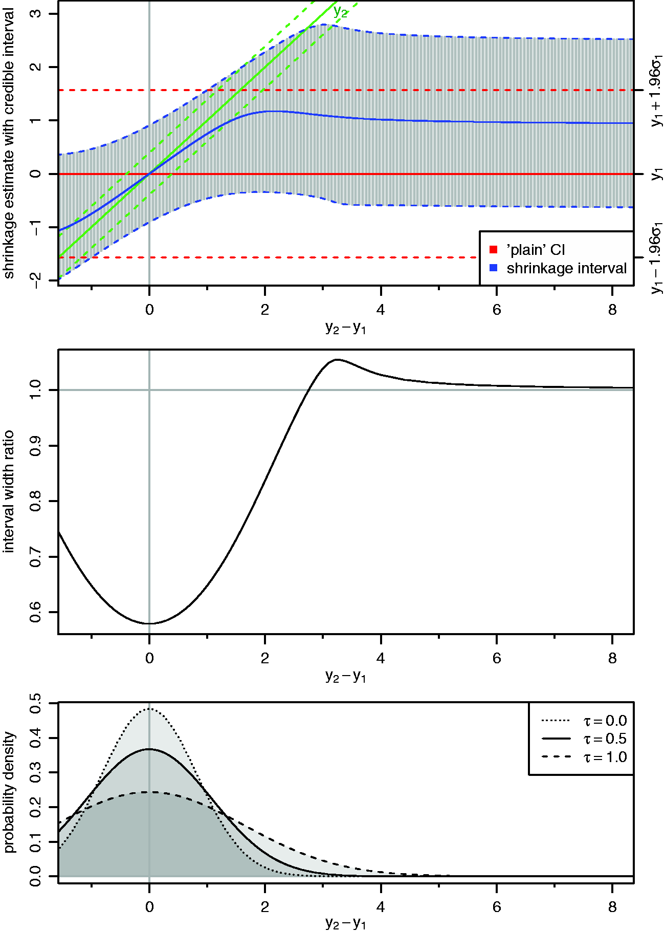 $y_{2} - y_{1}$ ) on the first shrinkage estimate (for θ₁). In the top row, one can see how the interval itself varies relative to the “plain” interval ( $y_{1} \pm 1.96 σ_{1}$ , red lines); the second estimate (y₂) and its corresponding CI are shown in green. The second row shows the ratio of interval lengths, and the bottom row shows the probability density of the actualized difference for selected values of τ. The heterogeneity prior used here for the analysis was half-normal (HN) with scale 0.5.

The middle panel shows that the shrinkage interval is shorter than the “plain” interval ( $y_{1} \pm 1.96 σ_{1}$ ) when the estimates y₁ and y₂ are similar, that it may also get wider in some cases, but that its width eventually is bounded. The bottom panel shows the probability distribution of the difference $y_{2} - y_{1}$ (which has variance $σ_{1}^{2} + σ_{2}^{2} + 2 τ^{2}$ ) for several selected values of τ. Based on the assumptions, the absolute difference is unlikely to exceed a value of, say, $| y_{2} - y_{1} | = 4$ , and so the probable cases essentially are those in the left half of the plot.

The scenario shown here is where we would in fact expect the greatest gain from considering the second estimate (y₂) in estimating θ₁, since the second estimate's error is much smaller than the first ( $σ_{2} << σ_{1}$ ). The figure looks qualitatively similar if we match or reverse the relative magnitudes of the standard errors σ₁ and σ₂, and also if we use a wider heterogeneity prior, but in those cases there is less information to be borrowed and hence less “shrinkage” taking place.

4 Simulation study

4.1 Setup

The simulations shown in the following are based on the NNHM, and since binary endpoints are very common in meta-analysis applications,³³ the setup is motivated by a scenario featuring a log-OR endpoint. If a study of size n_i results in a contingency table as an outcome, this may be converted into a log-OR that is associated with an approximate standard error of $σ_{i} = \frac{4}{\sqrt{n_{i}}}$ .²¹ A similar formula applies, for example, for logarithmic hazard ratios (log-HRs) from a survival analysis with respect to the event counts.²² In the following, we will consider combinations of “small”, “medium” and “large” studies of sizes $n_{i} \in {25, 100, 400}$ , corresponding to standard errors of $σ_{i} \in {0.8, 0.4, 0.2}$ . The true mean effect μ is (arbitrarily) fixed at zero. Analysis of a pair of studies will be based on a uniform prior for the effect μ, and a half-normal (HN) prior for the heterogeneity τ. Heterogeneity values in the range 0.5–1.0 may be considered as fairly high and above 1.0 as fairly extreme.²² A prior scale parameter of 0.5 already is a conservative choice, but in addition we also investigate the use of a HN(1.0) prior.^20,22 The true heterogeneity values in the simulation will be varied among $τ \in {0.0, 0.1, 0.2, 0.5, 1.0, 2.0}$ in order to check performance conditional on particular τ values. Similarly, we investigate the marginal performance by drawing τ according to the specified prior distribution. The primary interest will be in the first of the two studies ( $i = 1$ ) and especially the shrinkage estimate of its study-specific effect θ₁. The number of simulations for each scenario is 10,000.

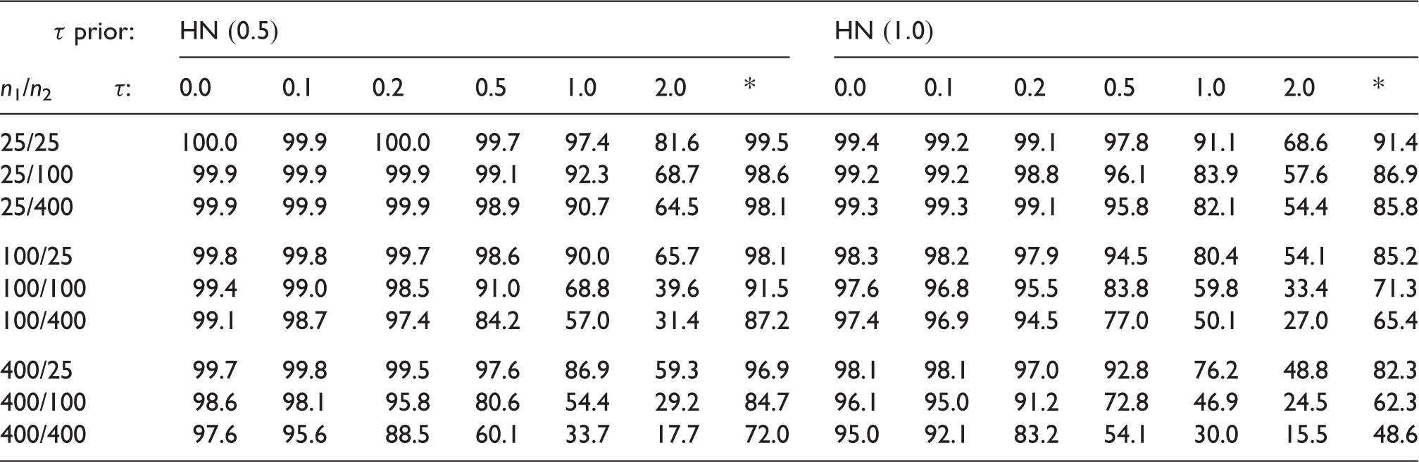
We can compare the resulting precision by comparing the 95% shrinkage interval width δ_i with the original confidence interval width and considering the relative width $q_{i} = \frac{δ_{i}}{2 \times 1.96 σ_{i}}$ . Assuming that standard errors scale with $n_{i}^{- 0.5}$ , we can then estimate the approximate gain in effective sample size as $q_{i}^{- 2} - 1$ . For example, if the shrinkage interval is only half as wide as the original interval, this precision gain corresponds to a roughly four-fold (300%) increase in sample size. If the interval is $q_{i} = 90 %$ as wide, then this corresponds to an approximate $q_{i}^{- 2} - 1 = 23 %$ increase. R code to reproduce the simulations is included in the supplement.

4.2 Coverage

Table 1 illustrates the coverage of shrinkage intervals for the effect θ₁ for different combinations of study sizes (n₁, n₂), heterogeneity values (τ) and heterogeneity priors (scales 0.5 and 1.0). The columns marked by an asterisk (*) correspond to the “marginal” simulations in which heterogeneity τ is not fixed, but varied according to the specified prior distribution. Coverages are close to or above the nominal 95% level, except if heterogeneity approaches a priori improbable large values. For the simulations in which τ is drawn from its prior distribution, we know that by definition the coverage would be exactly 95% if the effect μ was also drawn from its prior.³⁴ Since the effect prior is improper and μ was arbitrarily fixed at zero for the simulations, this only holds approximately here.

Table 1.

Coverage (%) of shrinkage intervals for estimation of the first study's mean parameter (θ₁).

τ prior:	$HN (0.5)$							$HN (1.0)$
n₁/n₂ $τ$ :	0.0	0.1	0.2	0.5	1.0	2.0	*	0.0	0.1	0.2	0.5	1.0	2.0	*
25/400	99.7	99.6	98.9	93.4	84.0	79.0	94.7	99.3	99.3	99.0	96.7	92.5	90.5	95.1
25/100	98.7	98.7	98.1	93.9	86.1	80.0	95.1	98.4	98.6	98.5	96.5	93.2	90.8	94.4
100/400	98.7	98.2	97.1	93.2	90.9	90.4	94.9	98.1	97.7	97.2	94.8	93.7	93.5	95.3
25/25	96.6	96.7	96.1	94.5	90.5	84.6	95.0	97.0	97.2	96.6	95.7	94.0	92.1	94.9
100/100	96.7	96.5	96.3	94.0	91.1	90.7	95.7	96.7	96.4	96.6	95.3	93.7	93.6	94.9
400/400	96.7	96.6	95.0	94.0	94.0	93.9	95.0	96.4	96.4	95.0	94.9	94.9	94.8	95.0
100/25	96.0	95.6	95.3	94.8	93.8	92.3	94.7	96.0	95.8	95.6	95.2	94.7	94.3	94.8
400/100	95.5	95.6	95.4	94.7	93.7	93.8	95.1	95.6	95.5	95.5	94.9	94.3	94.5	95.1
400/25	95.1	95.1	95.2	94.7	94.9	94.5	95.3	95.0	95.2	95.2	94.8	95.0	95.0	95.2

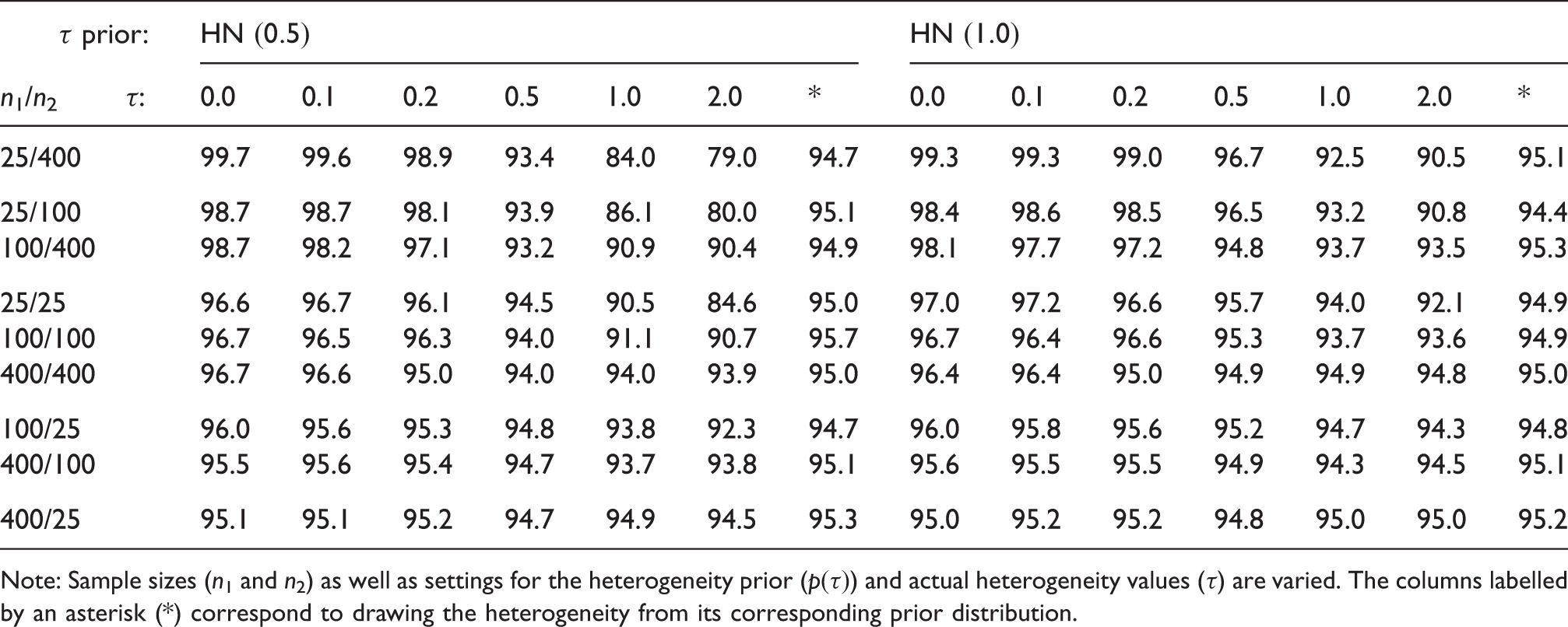
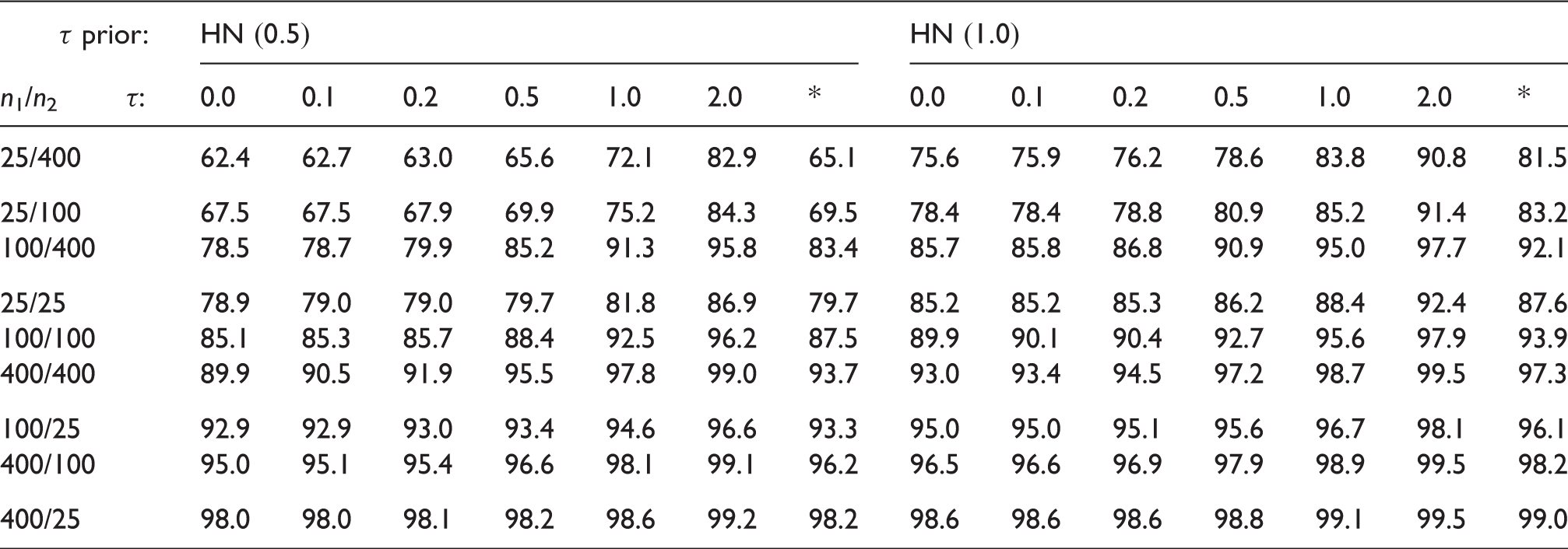
Note: Sample sizes (n₁ and n₂) as well as settings for the heterogeneity prior ( $p (τ)$ ) and actual heterogeneity values (τ) are varied. The columns labelled by an asterisk (*) correspond to drawing the heterogeneity from its corresponding prior distribution.

4.3 Interval length and effective sample size gain

Table 2 shows the mean lengths of shrinkage intervals relative to the original (“plain”) confidence interval based on y₁ and σ₁ alone (which has width

2 \times 1.96 σ_{1}

). While we have seen in the previous section that intervals may be shorter or longer in certain cases, here we see that on average the shrinkage intervals are always shorter than the plain intervals. As expected, the gain is largest if the study under consideration is small relative to the additional evidence (

n_{1} < n_{2}, σ_{1} > σ_{2}

), and if heterogeneity is low. Assuming a wider heterogeneity prior also reduces the amount of borrowing of information and leads to wider intervals.

Table 2.

Mean width (%) of shrinkage intervals (for θ₁) relative to original “plain” CI based only on y₁ and σ₁.

τ prior:	$HN (0.5)$							$HN (1.0)$
n₁/n₂ $τ$ :	0.0	0.1	0.2	0.5	1.0	2.0	*	0.0	0.1	0.2	0.5	1.0	2.0	*
25/400	62.4	62.7	63.0	65.6	72.1	82.9	65.1	75.6	75.9	76.2	78.6	83.8	90.8	81.5
25/100	67.5	67.5	67.9	69.9	75.2	84.3	69.5	78.4	78.4	78.8	80.9	85.2	91.4	83.2
100/400	78.5	78.7	79.9	85.2	91.3	95.8	83.4	85.7	85.8	86.8	90.9	95.0	97.7	92.1
25/25	78.9	79.0	79.0	79.7	81.8	86.9	79.7	85.2	85.2	85.3	86.2	88.4	92.4	87.6
100/100	85.1	85.3	85.7	88.4	92.5	96.2	87.5	89.9	90.1	90.4	92.7	95.6	97.9	93.9
400/400	89.9	90.5	91.9	95.5	97.8	99.0	93.7	93.0	93.4	94.5	97.2	98.7	99.5	97.3
100/25	92.9	92.9	93.0	93.4	94.6	96.6	93.3	95.0	95.0	95.1	95.6	96.7	98.1	96.1
400/100	95.0	95.1	95.4	96.6	98.1	99.1	96.2	96.5	96.6	96.9	97.9	98.9	99.5	98.2
400/25	98.0	98.0	98.1	98.2	98.6	99.2	98.2	98.6	98.6	98.6	98.8	99.1	99.5	99.0

The gain in precision may approximately be translated to an equivalent gain in effective sample size (as expressed through the q_i introduced above). The average gain is shown in Table 3. This relative gain in information may be substantial and is most pronounced if n₁ is small relative to n₂. For example, for the HN(0.5) heterogeneity prior and

n_{1} = 25

, we can expect a gain of at least one third across all scenarios, and even a gain of more than 100% is well achievable in certain cases. When averaging over the heterogeneity prior, i.e. if we assume the prior to accurately reflect the probability distribution for τ, we can expect a gain of more than 50% for the cases where

n_{1} = 25

and more than 100% when in addition

n_{2} > n_{1}

Table 3.

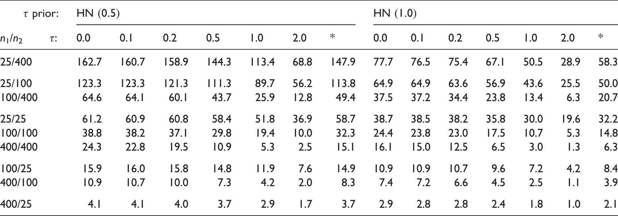
Gain (%) in effective sample size when using the shrinkage estimate, relative to the original CI.

τ prior:	$HN (0.5)$							$HN (1.0)$
n₁/n₂ τ:	0.0	0.1	0.2	0.5	1.0	2.0	*	0.0	0.1	0.2	0.5	1.0	2.0	*
25/400	162.7	160.7	158.9	144.3	113.4	68.8	147.9	77.7	76.5	75.4	67.1	50.5	28.9	58.3
25/100	123.3	123.3	121.3	111.3	89.7	56.2	113.8	64.9	64.9	63.6	56.9	43.6	25.5	50.0
100/400	64.6	64.1	60.1	43.7	25.9	12.8	49.4	37.5	37.2	34.4	23.8	13.4	6.3	20.7
25/25	61.2	60.9	60.8	58.4	51.8	36.9	58.7	38.7	38.5	38.2	35.8	30.0	19.6	32.2
100/100	38.8	38.2	37.1	29.8	19.4	10.0	32.3	24.4	23.8	23.0	17.5	10.7	5.3	14.8
400/400	24.3	22.8	19.5	10.9	5.3	2.5	15.1	16.1	15.0	12.5	6.5	3.0	1.3	6.3
100/25	15.9	16.0	15.8	14.8	11.9	7.6	14.9	10.9	10.9	10.7	9.6	7.2	4.2	8.4
400/100	10.9	10.7	10.0	7.3	4.2	2.0	8.3	7.4	7.2	6.6	4.5	2.5	1.1	3.9
400/25	4.1	4.1	4.0	3.7	2.9	1.7	3.7	2.9	2.8	2.8	2.4	1.8	1.0	2.1

4.4 Fraction of shortened intervals

While there is a gain on average, the shrinkage intervals may in some cases also turn out wider than the original interval. Table 4 shows the percentages of intervals showing a smaller width. In a majority of cases, we can expect a shorter interval, the exceptions are again cases where the heterogeneity is large, or the second study is small.

Table 4.

Fraction (%) of shrinkage intervals turning out shorter than the original CI. Note the differing ordering of rows compared to Tables 1 to 3.

τ prior:	$HN (0.5)$							$HN (1.0)$
n₁/n₂ τ:	0.0	0.1	0.2	0.5	1.0	2.0	*	0.0	0.1	0.2	0.5	1.0	2.0	*
25/25	100.0	99.9	100.0	99.7	97.4	81.6	99.5	99.4	99.2	99.1	97.8	91.1	68.6	91.4
25/100	99.9	99.9	99.9	99.1	92.3	68.7	98.6	99.2	99.2	98.8	96.1	83.9	57.6	86.9
25/400	99.9	99.9	99.9	98.9	90.7	64.5	98.1	99.3	99.3	99.1	95.8	82.1	54.4	85.8
100/25	99.8	99.8	99.7	98.6	90.0	65.7	98.1	98.3	98.2	97.9	94.5	80.4	54.1	85.2
100/100	99.4	99.0	98.5	91.0	68.8	39.6	91.5	97.6	96.8	95.5	83.8	59.8	33.4	71.3
100/400	99.1	98.7	97.4	84.2	57.0	31.4	87.2	97.4	96.9	94.5	77.0	50.1	27.0	65.4
400/25	99.7	99.8	99.5	97.6	86.9	59.3	96.9	98.1	98.1	97.0	92.8	76.2	48.8	82.3
400/100	98.6	98.1	95.8	80.6	54.4	29.2	84.7	96.1	95.0	91.2	72.8	46.9	24.5	62.3
400/400	97.6	95.6	88.5	60.1	33.7	17.7	72.0	95.0	92.1	83.2	54.1	30.0	15.5	48.6

4.5 Implications for practical application

The previous sections illustrate the process of shrinkage estimation within the NNHM framework and investigate the potential benefits. Across a range of realistic settings, the method exhibits sensible and robust behaviour, and despite the seemingly pathological outset of synthesizing only two estimates, the expected information gain may still be substantial. In the following, we will illustrate the approach by applying it in two examplary cases, one based on two studies (one randomized, one observational), and one based on two estimates from meta-analyses of different types of studies.

5 An application in Creutzfeld-Jakob disease

With a prevalence of 1 in $1, 000, 000$ ³⁵ and an incidence of 1.5 per million and year,³⁶ Creutzfeld-Jakob disease (CJD) is clearly a rare disease by any standard. In a recent systematic review, Unkel et al.³⁷ identified a number of shortcomings in the methodologies applied in clinical studies conducted in CJD and advocated the use of innovative statistical methodology including evidence synthesis approaches.

Varges et al.³ studied the use of doxycycline, an antiprion agent, in early CJD. They conducted a double-blind randomised placebo-controlled trial that failed to recruit the originally planned number of patients and was terminated prematurely with only n = 12 patients (seven on doxycycline and five on placebo). Additionally, data were available from an observational study of n = 88 patients including 55 patients who received doxycycline. The primary endpoint was all-cause mortality which was analyzed using Cox proportional hazard regressions. In the case of the randomized controlled trial, the model included only the factor treatment as independent variable whereas the analysis of the observational data in addition was stratified by propensity scores. The observed log hazard ratios (standard errors) were −0.173 (0.631) and −0.499 (0.249) in the randomized controlled trial and the observational study, respectively. Varges et al. performed a random-effects meta-analysis to estimate the overall (pooled) effect μ using standard frequentist methodology. They reported a combined hazard ratio of 0.633 with 95% confidence interval of $(0.402; 0.999)$ .

Now suppose primary interest was in the ‘randomized’ effect, but one is willing to utilize external observational evidence as supporting information. We may now apply the shrinkage estimation approach. Figure 2 shows the estimated logarithmic hazard ratios based on obervational and randomized data along with the derived mean estimate (μ). The two shrinkage estimates are also shown next to the original (quoted) estimates. For the randomized trial, the updated credible interval covers the range of [ $- 1.16, 0.48$ ] and is only 66% as wide as the original interval. This amount of shrinkage implies a gain in effective sample size of 129%, i.e. this corresponds to more than a doubling of the original sample size from 12 patients to an ‘effective number’ of some 27 patients. For the randomized patients’ shrinkage estimate, we then obtain a posterior probability of a non-beneficial effect of $P (θ_{rand .} > 0 | y) = 0.16$ . The associated (one-sided) posterior predictive p-value is similar, with p = 0.13.

Figure 2.

Forest plot for the CJD example (log-HR outcome). The shrinkage interval for the log-HR based on randomized evidence here is [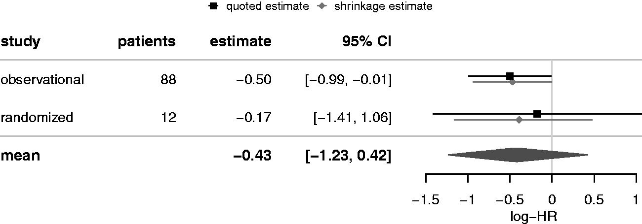 $- 1.16, 0.48$ ], spanning only two-thirds of the original confidence interval width.

From two studies, there is only very little to be learned about the between-study heterogeneity τ.²⁴ The prior median heterogeneity was at 0.34, which a posteriori is slightly reduced to 0.28; the posterior 95% quantile is at 0.85 instead of 0.98. Note that while the estimates for the overall mean and the shrinkage estimate do not differ much in this particular case, their interpretations are quite different. The R code to reproduce the calculations for this example is provided in Appendix 1.

6 Beyond two studies: more general shrinkage applications

So far we have described shrinkage estimation mostly in terms of “studies” and corresponding parameter estimates. However, the method may be applied more widely. Estimates do not need to come from studies, these could also originate from different types of evidence, for example, from two meta-analyses, or from a meta-analysis and a single study.

If the NNHM is fitted to the results of meta-analyses, then this adds another hierarchical level to the model. In the spirit of a bias allowance model framework,³⁸ in addition to between-study variability, the variability between study types is considered as a separate variance component. Especially in the context of normal models^39,40 and when interest is in main effects,⁴¹ application of a one-stage model simultaneously including all hierarchy levels may in many cases not lead to substantially different results from a simpler two-stage approach in which data at the study-level are combined first, and summaries are subsequently combined in a second stage.⁴² This way, inference is substantially simplified, and standard meta-analysis software can be used.

Consider the example of a meta-analysis investigating the effect of immunosuppression in paediatric patients, where the outcome of interest is the occurrence of acute rejection (AR) events that the therapy is supposed to prevent.⁴³ Only two randomized trials are available, but in addition four observational studies reported on the effect. One may not expect to see identical effects in both types of studies, but the discrepancy between them will be limited. A meta-analysis of the two randomized trials may then profit from considering the outcomes of the four observational trials in addition, leading to a particular kind of extrapolation approach.⁴⁴

Figure 3 shows the example data. In both sets of studies we see similar effects, the negative combined estimates of the log-odds-ratio indicate a successful prevention of AR events, and the two associated credible intervals are mostly overlapping. After combining the two sets of studies separately, we may now perform a meta-analysis of the resulting two combined estimates (in all cases using uniform priors for effects and HN(0.5) priors for heterogeneities). The shrinkage estimate for the mean effect in the randomized studies then provides an estimate for the randomized effect that is also informed by the observational evidence, while allowing for heterogeneity (at a second level) between both types of estimates. Note that in this context the shrinkage estimate then does not refer to a single study, but to one of the meta-analysis estimates that are combined here. The shrinkage estimate is shown at the very bottom of Figure 3. Compared to the original estimate based only on the two randomized trials, the shrinkage estimate is, in concordance with the observational evidence, slightly more moderate (at a lower absolute log-OR). Consideration of the additional evidence also gains precision: the shrinkage interval is 25% shorter than the original interval.

Figure 3.

Illustration of a more general shrinkage application. The two sources of evidence themselves here are meta-analyses of observational and randomized studies. The combined randomized estimate may then borrow information from the observational studies' evidence. The two combined estimates are again meta-analysed to yield a shrinkage interval for the randomized effect.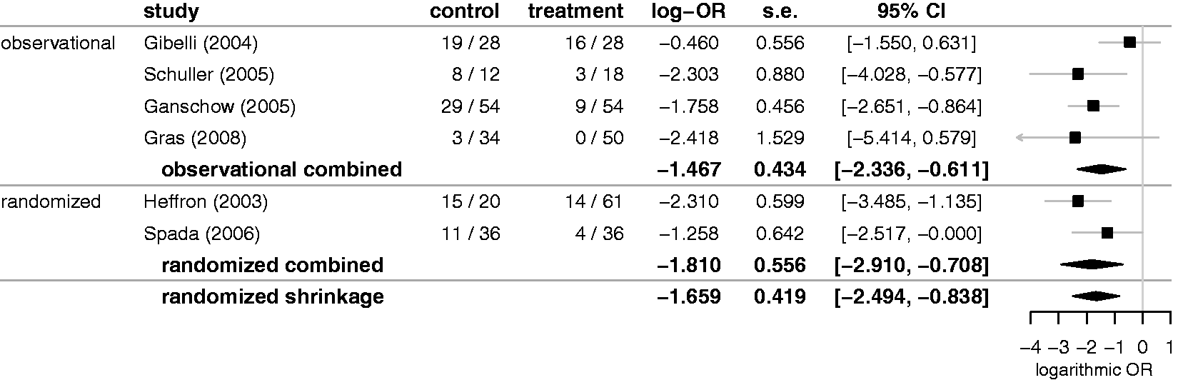

For the shrinkage estimate, we get a posterior probability of $P (θ_{rand .} > 0 | y) = 0.00007$ of a non-beneficial effect. With p = 0.0002, the associated posterior predictive p-value again is of a similar magnitude. Compared to the original meta-analysis of two randomized studies only, we can again see the gain in precision; here the evidence for a beneficial effect was not yet quite as pronounced ( $P (μ > 0 | y) = 0.0023$ and p = 0.0079). The R code to reproduce the calculations for this example is provided in Appendix 1.

7 Discussion

Use of the NNHM to consider external information via shrinkage estimation provides a transparent procedure based on well-defined parameters and a common model framework. The NNHM may readily be generalized, for example, to more studies, more levels of hierarchy, or the inclusion of regression parameters. The amount of information considered may be explicated by noting that a joint analysis is equivalent to the use of a meta-analytic-predictive (MAP) prior.¹¹ At the same time, heavy tails of the MAP prior ensure a certain degree of robustness of the shrinkage estimate in case of prior-data conflicts.³² The simulations demonstrate that the gain in precision may be greater than expected, and substantial especially in cases where the external data are associated with equal or less uncertainty than the data that are of primary interest. The possible precision gain may allow the conduct and evaluation of trials in circumstances where otherwise evidence would be too sparse, or it may generally enable to allocate resources more efficiently.

In the spirit of the reference model parametrization outlined above, the institution of an “overall mean” μ is not necessary. In many cases, when the data to be synthesized are of differing natures, the idea of a “central” mean parameter might be hard to motivate; what is relevant here is that the two estimates are modeled as being connected via an uncertain normally distributed offset. Normality here especially implies symmetry, i.e. the displacement between the two does not have a preferred direction; over- or under-estimation of one another are equally likely, so that a priori no systematic bias is assumed. Availability of this alternative motivation broadens the range of applicability of meta-analytic methods.

As usual, the user needs to be aware of the limits of the applicability of the model, which here in particular means that the normality assumptions should be plausible.⁴⁵ These assumptions might be challenged, for example, when estimates are based on count data suffering from small-sample or rare-event problems, in which case more specific models may be more appropriate.⁴⁶ We also make the implicit assumption that patient populations are sufficiently similar to allow for a meaningful comparison. Furthermore, analyses of non-randomized studies may need to be adjusted for confounding,^47,48 as was also done in the CJD example.

Although frequentist analyses still dominate clinical trials, examples of Bayesian analyses are emerging. A recent application is the trial by Laptook et al.⁴⁹ in newborns with hypoxic-ischemic encephalopathy, a form of brain damage resulting from an insufficient supply of oxygen to the brain. The authors used the Bayesian framework to interpret their results in the light of different choices of priors that they termed “neutral”, “skeptical” and “optimistic”.⁵⁰ In this regard, it differs from our proposal as we advocate the use of external data to inform the prior. The connection to common meta-analysis methods then helps motivating the choice of model details. Sensitivity analyses could be performed in our setting by varying the prior on the between-trial heterogeneity τ, for example, by varying the scale parameter of the half-normal prior.

Although not assessed in the simulations here, the performance of frequentist shrinkage BLUP estimators is likely to be unsatisfactory when dealing with only two studies. The reason lies in the underestimation of the between-study heterogeneity with a high likelihood of the variance estimate resulting in zero, and the challenge to incorporate the uncertaintly in the estimation of the heterogeneity in the inference.^20,24,51 A Bayesian alternative was described here and shown in simulations to have satisfactory properties under practically relevant scenarios. Therefore, the approach described here adds to the tool box of practicing statisticians. The proposed Bayesian approach can easily be implemented using the R package bayesmeta^21,26 and relevant code is provided as appendices for the two-study and the two-meta-analyses cases. The code to reproduce the simulations is also provided in the online supplement. The availability of posterior predictive p-values may aid in the interpretation of the findings. Furthermore, the efficient implementation facilitates sensitivity analyses and the assessment of operation characteristics of the procedures through simulations in so-called clinical scenario evaluations.⁵²

Footnotes

Declaration of conflicting interests

The author(s) declared no potential conflicts of interest with respect to the research, authorship, and/or publication of this article.

Funding

The author(s) disclosed receipt of the following financial support for the research, authorship, and/or publication of this article: This research has received funding from the EU's 7th Framework Programme for research, technological development and demonstration under grant agreement number FP HEALTH 2013-602144 with project title (acronym) “Innovative methodology for small populations research” (InSPiRe).

Appendices 1. R code for CJD example

References

Chataway

Friede

. The N-MOmentum trial: building momentum to advance trial methodology in a rare disease. Multiple Sclerosis J 2016; 22: 852–853.

Messroghli

Pickardt

Fischer

, et al. Toward evidence-based diagnosis of myocarditis in children and adolescents: rationale, design, and first baseline data of MYKKE, a multicenter registry and study platform. Am Heart J 2017; 187: 133–144.

Varges

Manthey

Heinemann

, et al. Doxycycline in early CJD – a double-blinded randomized phase II and observational study. J Neurol Neurosurg Psychiatry 2017; 88: 119–125.

Abrahamyan

Feldman

Tomlinson

, et al. Alternative designs for clinical trials in rare diseases. Am J Med Genet Part C (Seminars in Medical Genetics) 2016; 172: 313–331.

Hampson

Whitehead

Eleftheriou

, et al. Bayesian methods for the design and interpretation of clinical trials in very rare diseases. Stat Med 2014; 33: 4186–4201.

Thall PF, Ursino M, Baudouin V, et al. Bayesian treatment comparison using parametric mixture priors computed from elicited histograms. Stat Meth Med Res 2019; 28: 404–418.

Johnson

Tomlinson

Hawker

, et al. A valid and reliable belief elicitation method for Bayesian priors. J Clin Epidemiol 2010; 63: 370–383.

Viele

Berry

Neuenschwander

, et al. Use of historical control data for assessing treatment effects in clinical trials. Pharmaceut Stat 2014; 13: 41–54.

Pocock

. The combination of randomized and historical controls in clinical trials. J Chronic Dis 1976; 29: 175–188.

10.

Schoenfeld

Zheng

Finkelstein

. Bayesian design using adult data to augment pediatric trials. Clin Trials 2009; 6: 297–304.

11.

Schmidli

Gsteiger

Roychoudhury

, et al. Robust meta-analytic-predictive priors in clinical trials with historical control information. Biometrics 2014; 70: 1023–1032.

12.

Wandel

Neuenschwander

Röver

, et al. Using phase II data for the analysis of phase III studies: an application in rare diseases. Clinical Trials 2017; 14: 277–285.

13.

Hedges

Olkin

. Statistical methods for meta-analysis, San Diego, CA: Academic Press, 1985.

14.

Hartung

Knapp

Sinha

. Statistical meta-analysis with applications, Hoboken, NJ: John Wiley & Sons, 2008.

15.

Borenstein

Hedges

Higgins

JPT

, et al. Introduction to meta-analysis, Chichester, UK: John Wiley & Sons, 2009. .

16.

Gelman

Carlin

Stern

, et al. Bayesian data analysis, 3rd ed. Boca Raton, FL: Chapman & Hall/CRC, 2014.

17.

Raudenbush

Bryk

. Empirical Bayes meta-analysis. J Education Behaviour Stat 1985; 10: 75–98.

18.

Viechtbauer

. Conducting meta-analyses in R with the metafor package. J Stat Software 2010, pp. 36: 1–48, .

19.

Robinson

. That BLUP is a good thing: the estimation of random effects. Statistical Science 1991; 6: 15–32.

20.

Friede

Röver

Wandel

, et al. Meta-analysis of few small studies in orphan diseases. Res Synthesis Meth 2017; 8: 79–91.

21.

Röver C. Bayesian random-effects meta-analysis using the bayesmeta R package. arXiv preprint 1711.08683 2017, http://www.arxiv.org/abs/1711.08683 (accessed 10 October 2018).

22.

Spiegelhalter

Abrams

Myles

. Bayesian approaches to clinical trials and health-care evaluation, Chichester, UK: John Wiley & Sons, 2004. .

23.

Röver

Friede

. Contribution to the discussion of “When should meta-analysis avoid making hidden normality assumptions?”: a Bayesian perspective. Biometric J 2018; 60: 1068–1070.

24.

Friede

Röver

Wandel

, et al. Meta-analysis of two studies in the presence of heterogeneity with applications in rare diseases. Biometric J 2017; 59: 658–671.

25.

Gelman

. Prior distributions for variance parameters in hierarchical models. Bayesian Analysis 2006; 1: 515–534.

26.

Röver C. bayesmeta: Bayesian random-effects meta analysis, 2015. R package, http://cran.r-project.org/package=bayesmeta (accessed 11 October 2018).

27.

Meng

. Posterior predictive p-values. Ann Stat 1994; 22: 1142–1160.

28.

Gelman

Meng

Stern

. Posterior predictive assessment of model fitness via realized discrepancies. Statistica Sinica 1996; 6: 733–760. http://www.jstor.org/stable/24306036 .

29.

Gelman

. Two simple examples for understanding posterior p-values whose distributions are far from uniform. Electronic J Stat 2013; 7: 2595–2602.

30.

Neuenschwander

Roychoudhuri

Schmidli

. On the use of co-data in clinical trials. Stat Biopharmaceut Res 2016; 8: 345–354.

31.

Ibrahim

Chen

. Power prior distributions for regression models. Statistical Science 2000; 15: 46–60.

32.

O'Hagan

Pericchi

. Bayesian heavy-tailed models and conflict resolution: A review. Brazilian J Probabil Stat 2012; 26: 372–401.

33.

Davey

Turner

Clarke

, et al. Characteristics of meta-analyses and their component studies in the Cochrane Database of Systematic Reviews: a cross-sectional, descriptive analysis. BMC Med Res Methodol 2011; 11: 160.

34.

Gneiting

Balabdaoui

Raftery

. Probabilistic forecasts, calibration and sharpness. J Royal Stat Soc B 2007; 69: 243–268.

35.

National Institute of Neurological Disorders and Stroke (NINDS). Creutzfeldt-Jakob disease fact sheet. Technical Report NIH publication no. 03-2760. Bethesda, MD: National Institutes of Health, 2003, http://www.ninds.nih.gov/disorders/cjd/detail_cjd.htm.

36.

Wakap

Demarest

Lanneau

. Prevalence of rare diseases: bibliographic data. Orphanet Report Series, Rare Diseases Collection 2016, pp. 1.

37.

Unkel

Röver

Stallard

, et al. Systematic reviews in paediatric multiple sclerosis and Creutzfeldt-Jakob disease exemplify shortcomings in methods used to evaluate therapies in rare conditions. Orphanet J Rare Dis 2016; 11: 16.

38.

Welton

Sutton

Cooper

, et al. Evidence synthesis for decision making in healthcare, Chichester, UK: Wiley, 2012.

39.

Burke

Ensor

Riley

. Meta-analysis using individual participant data: one-stage and two-stage approaches, and why they may differ. Stat Med 2017; 36: 855–875.

40.

Morris TP, Fisher DJ, Kenward MG, et al. Meta-analysis of Gaussian individual patient data: two-stage or not two-stage? Stat Med 2018; 37: 1419–1438.

41.

Kontopantelis E. A comparison of one-stage vs two-stage individual patient data meta-analysis methods: a simulation study. Res Synthesis Meth 2018; 9: 417–430.

42.

Stewart

Tierney

. To IPD or not to IPD? Advantages and disadvantages of systematic reviews using individual patient data. Eval Health Professions 2002; 25: 76–97.

43.

Crins

Röver

Goralczyk

, et al. Interleukin-2 receptor antagonists for pediatric liver transplant recipients: a systematic review and meta-analysis of controlled studies. Pediatric Transplant 2014; 18: 839–850.

44.

Röver C, Wandel S and Friede T. Model averaging for robust extrapolation in evidence synthesis. Stat Med 2019; 38: 674–694.

45.

Jackson D and White IR. When should meta-analysis avoid making hidden normality assumptions? Biometric J 2018; 60: 1040–1058.

46.

Jackson

Law

Stijnen

, et al. A comparison of seven random-effects models for meta-analyses that estimate the summary odds ratio. Stat Med 2018; 37: 1059–1085.

47.

Schmoor

Caputo

Schumacher

. Evidence from nonrandomized studies: a case study on the estimation of causal effects. Am J Epidemiol 2008; 167: 1120–1129.

48.

Signorovitch

, et al. Comparative effectiveness without head-to-head trials. PharmacoEconomics 2010; 28: 935–945.

49.

Laptook

Shankaran

Tyson

, et al. Effect of therapeutic hypothermia initiated after 6 hours of age on death or disability among newborns with hypoxic-ischemic encephalopathy. J Am Med Assoc 2017; 318: 1550–1560.

50.

Quintana

Viele

JLR

. Bayesian analysis: using prior information to interpret the results of clinical trials. J Am Med Assoc 2017; 318: 1605–1606.

51.

Bender

Friede

Koch

, et al. Methods for evidence synthesis in the case of very few studies. Res Synthesis Meth 2018; 9: 382–392.

52.

Benda

Branson

Maurer

, et al. Aspects of modernizing drug development using clinical scenario planning and evaluation. Therapeutic Innovation Regulat Sci 2010; 44: 299–315.

Dynamically borrowing strength from another study through shrinkage estimation

Abstract

Keywords

1 Introduction

2 Statistical model and shrinkage estimation

2.1 The normal–normal hierarchical model

2.2 Shrinkage estimation

2.3 The Bayesian approach to meta-analysis

2.4 Posterior predictive p-values

2.5 The reference model as an alternative variation of the NNHM

3 Dependency of the shrinkage estimate on the observed heterogeneity

4 Simulation study

4.1 Setup

4.2 Coverage

4.3 Interval length and effective sample size gain

4.4 Fraction of shortened intervals

4.5 Implications for practical application

5 An application in Creutzfeld-Jakob disease

6 Beyond two studies: more general shrinkage applications

7 Discussion

Footnotes

Declaration of conflicting interests

Funding

Appendices 1. R code for CJD example

References