
Abstract
Hierarchical models such as the bivariate and hierarchical summary receiver operating characteristic (HSROC) models are recommended for meta-analysis of test accuracy studies. These models are challenging to fit when there are few studies and/or sparse data (for example zero cells in contingency tables due to studies reporting 100% sensitivity or specificity); the models may not converge, or give unreliable parameter estimates. Using simulation, we investigated the performance of seven hierarchical models incorporating increasing simplifications in scenarios designed to replicate realistic situations for meta-analysis of test accuracy studies. Performance of the models was assessed in terms of estimability (percentage of meta-analyses that successfully converged and percentage where the between study correlation was estimable), bias, mean square error and coverage of the 95% confidence intervals. Our results indicate that simpler hierarchical models are valid in situations with few studies or sparse data. For synthesis of sensitivity and specificity, univariate random effects logistic regression models are appropriate when a bivariate model cannot be fitted. Alternatively, an HSROC model that assumes a symmetric SROC curve (by excluding the shape parameter) can be used if the HSROC model is the chosen meta-analytic approach. In the absence of heterogeneity, fixed effect equivalent of the models can be applied.
Keywords
1 Introduction
Meta-analysis of test accuracy studies aims to produce reliable evidence about the diagnostic accuracy of a medical test from multiple studies addressing the same question. The bivariate model 1 and the hierarchical summary receiver operating characteristic (HSROC) model 2 are the two approaches recommended for meta-analysis when a sensitivity and specificity pair is available for each study.3–5 These hierarchical models possess theoretical advantages over simpler methods for meta-analysis of test accuracy studies but fitting them is not trivial. The models are often fitted using a frequentist approach that relies on likelihood based methods for the estimation of five parameters. Solving the likelihood equations requires an iterative process and in certain circumstances, for instance when there are few studies and/or sparse data (e.g. zero cells due to perfect sensitivity and/or specificity) in a meta-analysis, the models fail to converge or they converge but give unreliable parameter estimates with one or more missing standard errors. These issues are often encountered by meta-analysts 6 and there is uncertainty about how to proceed with meta-analysis in such situations.
Academic illustrations of the application of hierarchical methods have typically involved large meta-analyses.1,2,4,7–13 In contrast, our experience of supporting Cochrane and non-Cochrane diagnostic test accuracy review authors suggest that small meta-analyses or sparse data often occur and pose a challenge to these data hungry hierarchical models. Others have also noted the problem of non-convergence.8,10,14–16 Despite the increasing uptake of these models, a recent survey has suggested a lack of clarity about recommended methods for meta-analysis and a need for guidance. 16 In this paper, using simulation, we evaluate the performance of hierarchical models for meta-analysis of diagnostic accuracy studies, and we develop recommendations for their use. Because sensitivity and specificity are the test accuracy measures most commonly used in meta-analyses, 17 we consider only methods for synthesis of these measures. Other measures such as likelihood ratios can be derived from functions of the bivariate or HSROC model parameters.
The outline of this paper is as follows. In section 2 we briefly describe common methods used for meta-analysis when each study contributes a single 2 x 2 table of the results of an index test cross classified with a reference standard. In section 3 we outline two motivating examples where the bivariate model failed to converge, and we apply simpler forms of the hierarchical models to resolve this. In section 4 we describe the simulation study and present the results for full and simplified hierarchical models. In section 5 we discuss our findings and conclude with recommendations for selecting an appropriate meta-analytic approach in practice.
2 Methods for meta-analysis of diagnostic accuracy studies
2.1 Univariate pooling methods
Univariate fixed effect or random effects meta-analytic methods pool sensitivity and specificity separately, ignoring any correlation that may exist between the two measures. Fixed effect models assume homogeneity while random effects models assume variability in test accuracy beyond sampling error alone by allowing each study to have its own test accuracy, i.e. the model includes a between study variance component (

2.2 Summary receiver operating characteristic regression
The summary receiver operating characteristic (SROC) curve approach developed by Moses et al. 18 accounts for possible heterogeneity in threshold. It uses a logistic transformation of the true positive and false positive rates (TPR and FPR) and linear regression to model the relationship between test accuracy and the proportion test positive (related to threshold). If accuracy does not depend on threshold, the SROC curve is symmetric and can be described by a constant diagnostic odds ratio (DOR). The DOR is a single measure of test accuracy defined as the ratio of the odds of positivity in those who have the target condition relative to the odds of positivity in those without the condition. Therefore, a test with high TPR and low FPR will have a high DOR. This SROC approach is a fixed effect method in which variation is attributed solely to threshold effect and sampling error. The approach has methodological limitations which lead to inaccurate standard errors, thus rendering formal statistical inference invalid.10,13 Similar to the DerSimonian and Laird approach, zero cell corrections may be required.
2.3 Hierarchical models
Hierarchical models (also known as mixed or multilevel models) take into account correlation between sensitivity and specificity across studies while also allowing for variation in test performance between studies through the inclusion of random effects. The two main approaches – the bivariate model and the HSROC model – differ in parameterizations, but the models are mathematically equivalent when no covariates are included. 19 The choice of approach is often determined by variation in the thresholds reported in the included studies and the focus of inference – a summary point or a SROC curve.
2.3.1 Bivariate random effects model
van Houwelingen et al.
20
proposed a bivariate approach to meta-analysis that was adapted by Reitsma et al.
1
for test accuracy meta-analysis. This bivariate model is a linear mixed model that enables joint analysis of sensitivity and specificity and takes the form


2.3.2 HSROC model
The Rutter and Gatsonis HSROC model represents a general framework for meta-analysis of test accuracy studies and can be viewed as an extension of the Moses SROC approach in which the TPR and FPR for each study are modelled directly.
21
The HSROC model is a nonlinear generalized mixed model and takes the form

3 Motivating examples
3.1 Non-contrast computed tomography for diagnosing appendicitis
Hlibczuk et al.
23
reviewed the diagnostic accuracy of non-contrast computed tomography (CT) for emergency department evaluation of adults with suspected appendicitis. Seven studies, evaluating 1060 patients of whom 389 had appendicitis, were included in the review. The prevalence of appendicitis in the studies ranged from 20% to 84%, with a median of 39%. The forest plot (Figure 1) shows between study variation in the sensitivities and specificities, though specificity was perfect (100%) in four studies. The authors attempted to fit the bivariate model in SAS but the model failed to converge.
Forest plot of sensitivity and specificity estimates from studies included in the two motivating examples. FN: false negative; FP: false positive; TN: true negative; TP: true positive.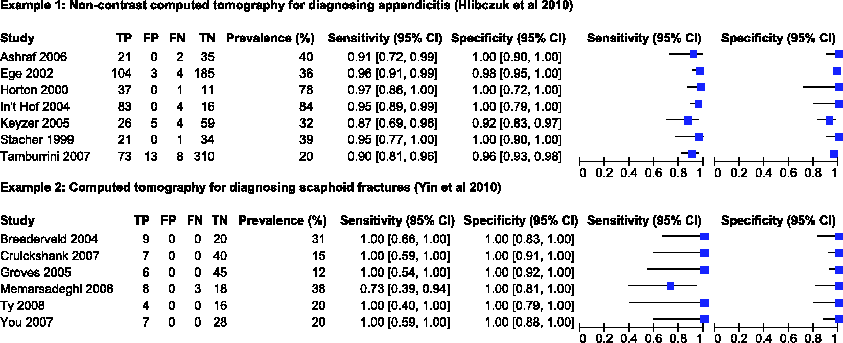
3.2 CT for diagnosing scaphoid fractures
Yin et al. 24 assessed the diagnostic accuracy of CT for diagnosing suspected scaphoid fractures. Six studies, evaluating 211 patients of whom 44 had a scaphoid fracture, were included in the review. The prevalence of scaphoid fractures in the studies ranged from 12% to 38%, with a median of 20%. Figure 1 shows the estimates of sensitivity and specificity with almost no between study variation; five of the six studies reported 100% sensitivity while all studies reported 100% specificities. The authors pooled sensitivity, specificity and the DOR using a random effects model (method not specified).
3.3 Results from reanalysis of the two example datasets
Summary accuracy measures obtained from different meta-analytic models applied to the two motivating examples.
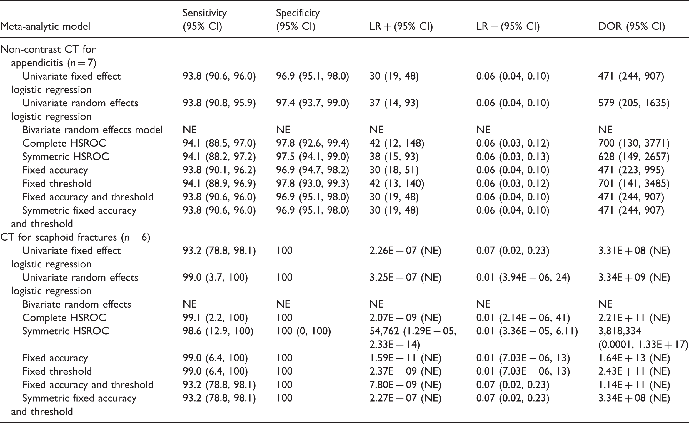
n: number of studies in the meta-analysis, NE: not estimable.
Since the maximum likelihood estimation problems encountered with the bivariate model are most likely due to boundary estimation of the variance and/or covariance parameters, we attempted plotting the profile log likelihood for the covariance parameter (maximized with respect to the other 4 parameters). We were unable to produce a plot for the scaphoid fracture example because the bivariate model failed even with fixed values for the covariance. This is unsurprising since there was almost no between study variation in sensitivity and specificity.
Figure 2 shows the profile log likelihood for the covariance parameter for the appendicitis example. The likelihood is flat with very little change in the profile log likelihood. The maximum of the profile log likelihood was achieved at a covariance of 0.02 (dashed line). For covariances above 0.02, the bivariate model failed to converge or was unstable, but values between −0.05 and 0.02 appear to be supported by the data. The dotted line shows the value of the log likelihood for a covariance of zero, i.e. independence between sensitivity and specificity. This suggests that UREMs would be appropriate for pooling sensitivity and specificity in this example.
Profile log-likelihood function of the covariance parameter in the bivariate model applied to the appendicitis example.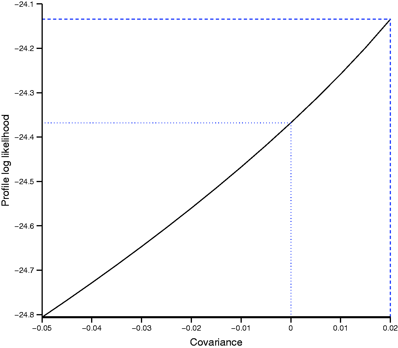
The two examples illustrate the problem of model convergence, poor parameter estimation and the need for simpler models. There were only subtle differences in summary estimates and 95% CIs for sensitivity, specificity and the negative likelihood ratio between models fitted to the appendicitis dataset. In contrast, clear differences were observed for the positive likelihood ratio and the DOR. For the scaphoid fractures dataset, there were differences in summary estimates and 95% CI for sensitivity and specificity from the univariate fixed effect model and the HSROC models with both fixed accuracy and threshold parameters compared to the other models. These examples show that results can differ between models, and the differences may not be negligible. Therefore, the identification of simpler meta-analytic methods that give valid answers in situations where complex models fail is of practical importance.
4 Simulation study
4.1 Simulation methods
We conducted a simulation study to compare the performance of a UREM and the HSROC model with various simplifications (by removing model parameters). Given the mathematical equivalence of the HSROC and bivariate models when no covariate is included, there was no need to examine the performance of both models. We chose the HSROC model because it has greater flexibility for introducing model parsimony by dropping parameters than the bivariate model. 19 Since several authors7–9,15 have shown that approximate methods for modelling within study variability are biased, we only investigated methods that use a binomial likelihood. The specifications for the scenarios were devised to replicate realistic situations encountered in meta-analysis of diagnostic accuracy studies. We investigated the effect of these factors: 1) number of studies; 2) magnitude of diagnostic accuracy (DOR); 3) prevalence of disease; 4) between study variation in accuracy and threshold; and 5) asymmetry in the SROC curve. We modified the simulation approach used in a previous study 25 to define the simulation scenarios and generate the simulated datasets as described below.
4.1.1 Generation of simulated data
To determine diagnostic accuracy, we used the standardised distance between the means 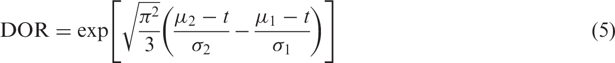
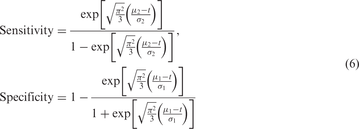
For scenarios where
We investigated meta-analyses with different number of studies (k = 5, 10, 20). The size of a study in each meta-analysis, nj, was randomly sampled from a uniform distribution, U(20,200). We varied nj between 20 and 200 because diagnostic accuracy studies are often small in size.17,26 Given an underlying prevalence p, individuals within each study were randomly classified as diseased or non-diseased, and assigned a continuous test result value, x, which was randomly sampled from the logistic distributions. For each study, we used t to determine the outcome of an individual's test result; positive if
Scenarios evaluated in the simulation. a
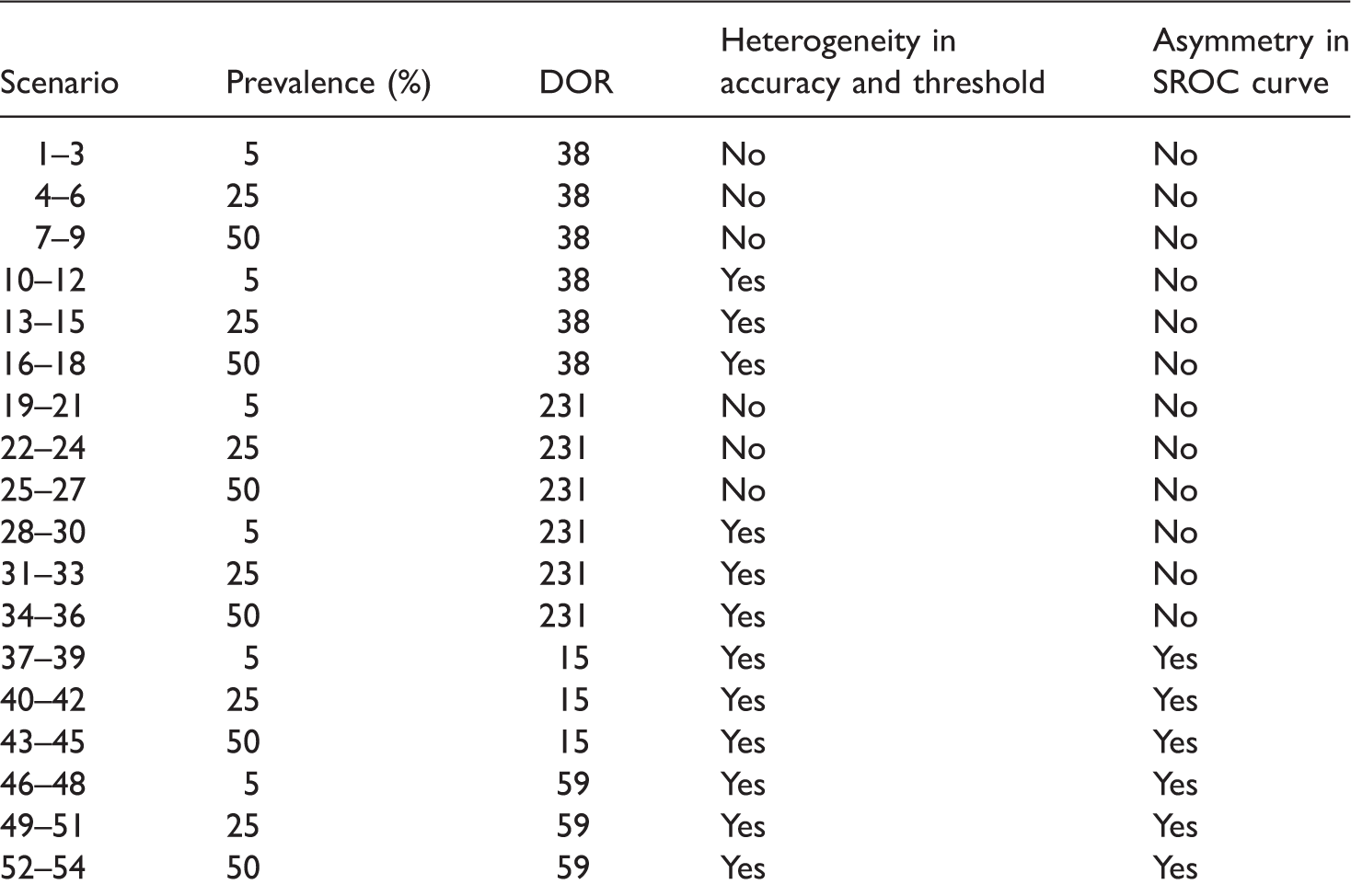
Each subset of 3 scenarios corresponds to 5, 10 and 20 studies.
4.1.2 Meta-analytic models fitted to each dataset
Throughout the rest of this paper, we refer to an HSROC model that contained all five parameters as a complete HSROC model. We fitted the following seven models to each meta-analysis dataset.
UREM – includes Complete HSROC model – includes all five parameters Λ, Θ, β, Symmetric HSROC model – includes Λ, Θ, HSROC model with fixed threshold – includes Λ, Θ, β and HSROC model with fixed accuracy – includes Λ, Θ, β and HSROC model with fixed accuracy and threshold – includes Λ, Θ and β (allows for asymmetry in the SROC curve) Symmetric HSROC model with fixed accuracy and threshold parameters – includes only two parameters Λ and Θ
As shown by Harbord et al.,
19
the five parameters of the bivariate model can be expressed in terms of those of the HSROC model as follows:


4.1.3 Facilitating convergence of hierarchical models
To aid convergence, we provided a wide range of starting values for model parameters by specifying a grid of points for a grid search of starting values. We used a quasi-Newton optimization technique (the NLMIXED default) because it provides an appropriate balance between computation speed and stability (SAS Institute Inc. SAS OnlineDoc® 9.1.3. Cary, NC, 2004). To prevent estimation of negative variances and to reduce computational problems, we specified boundary constraints (σ2 ≥ 0) for the variance parameters in the models. To reduce the number of models that failed to converge, we refitted models by trying a new set of starting values and/or changing the optimization technique to a Newton-Raphson technique. To obtain a new set of starting values, we fitted a model with no random effects and used the new parameter estimates together with the original grid of points for the variance parameters. Thus for some datasets, we made up to four attempts to fit a hierarchical model.
4.1.4 Assessment of model convergence and stability
Because a model that meets a convergence criterion may be unstable or have missing standard errors due to issues with model identifiability, we assessed convergence in two stages. First, we checked whether the convergence criterion was met and also whether the additional estimates defined in the ESTIMATE statements were produced. Second, because standard errors are computed from the final Hessian matrix, we calculated eigenvalues of the Hessian to detect if there were problems. At a true minimum, eigenvalues will all be positive, i.e. positive definite. Therefore, for convergence to be deemed successful, the model had to meet the convergence criterion, produce additional estimates, and the Hessian had to be positive definite.
4.1.5 Assessment of performance of meta-analytic models
We assessed performance of the methods by examining estimates of the following measures of diagnostic accuracy: log DOR, logit sensitivity and logit specificity. We assessed estimability as the percentage of meta-analyses that successfully converged and the percentage where the between study correlation was not estimated as −1 or +1. We computed the latter for only the complete HSROC model. For each scenario, we used only the results from meta-analyses that successfully converged as defined above to calculate (a) the difference between the average parameter estimate and the true parameter value to determine bias; (b) the average standard error and mean square error (MSE incorporates both bias and variability) to assess model accuracy; and (c) the coverage of the 95% CIs by computing the percentage of meta-analyses for which the true parameter value was within the 95% CI.
4.2 Simulation results
Altogether we explored 54 scenarios. We can only show results for the log DOR in this article but results for logit sensitivity and logit specificity are briefly mentioned. Because homogeneous accuracy and threshold are the exception rather than the norm for meta-analysis of test accuracy studies, to illustrate key findings, we present results mainly for scenarios with heterogeneity at a DOR of 231 (sparse data are of interest and zero false positives and/or false negatives are more likely to occur when diagnostic accuracy is high).
4.2.1 Estimability
Convergence and estimability of the complete HSROC model applied to 10,000 datasets in 36 different scenarios. a
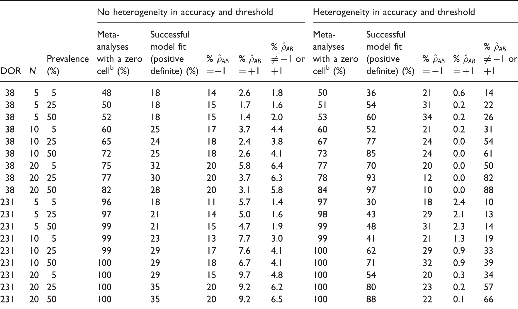
All results are presented as percentages and are based on 10,000 meta-analysis datasets.
The percentage of meta-analyses out of 10,000 where at least one study included a zero cell.
Performance of all meta-analytic models in estimating the log DOR for scenarios with a DOR of 231.

DOR: diagnostic odds ratio; FA: fixed accuracy HSROC model; FAT: fixed accuracy and threshold HSROC model; FT: fixed threshold HSROC model; MSE: mean square error; N: number of meta-analyses out of 10,000 where hierarchical models successfully converged; SFAT: symmetric fixed accuracy and threshold HSROC model; UREM: univariate random effects logistic regression model.
Heterogeneity in accuracy and threshold.
Bias is presented as a percentage of the true value of the log diagnostic odds ratio.
4.2.2 Bias
In the base scenario for a DOR of 231, the symmetric HSROC model gave the least percentage bias for the DOR (4.32%); bias was highest for the fixed threshold (37.8%) and fixed accuracy (36.2%) models (Table 4). These rankings were consistent as the number of studies increased. As prevalence increased, the two fixed effect models became the least biased while the fixed accuracy model remained the most biased.
When heterogeneity was introduced, each of the seven models produced the largest bias for the DOR at the lowest prevalence, though the univariate random effects model gave the least biased DOR. For all models, bias decreased as prevalence and the number of studies increased. However, the decrease in bias resulted in a change from overestimation to underestimation for the two fixed effect models. For bias in the estimates of sensitivity, we observed results similar to those of the DOR, but the relationship with prevalence was reversed for bias in the estimates of specificity (data not shown). Bias in specificity was very small compared to that of the DOR or sensitivity. For the three measures, in scenarios with heterogeneity and asymmetry in the SROC curve, bias was lower than in the corresponding symmetric model.
4.2.3 Model accuracy
A MSE of zero indicates that the model estimated the parameter of interest with perfect accuracy, i.e. no bias and no variability in the estimation. The MSE of the DOR was highest for the symmetric fixed accuracy threshold model (40.7) but lowest for the symmetric HSROC model (4.26) in the base scenario (Table 4). At higher prevalence, the two fixed effect models had the lowest MSE. For all models, the MSE of the DOR decreased as the number of studies and prevalence increased. When heterogeneity was introduced, the univariate random effects model had the lowest MSE at 5% prevalence but the symmetric HSROC model had slightly lower MSE than the univariate random effects model at higher values of prevalence. As the number of studies and prevalence increased, the MSE for all models decreased and became almost identical except for those of the two fixed effect models. Results for sensitivity were similar to those for the DOR. The MSE for specificity was generally very low and increased slightly with increasing prevalence. For the asymmetric SROC curve scenarios, the findings for the three measures were similar to those of the corresponding symmetric scenarios.
4.2.4 Coverage
For a DOR of 231, the symmetric HSROC models gave the best coverage of the 95% CIs for estimation of the DOR (95.5%) in the base scenario. With the exception of the symmetric fixed accuracy threshold model, all models were conservative as shown by coverage greater than 95%. The coverage of 88% for the symmetric fixed accuracy threshold model implied over-confidence in the estimates but coverage increased as prevalence or the number of studies increased. In contrast, introduction of heterogeneity led to very poor coverage for the two fixed effect models with coverage becoming lower as prevalence increased. The univariate random effects model and symmetric HSROC model often showed good coverage, although the latter tended to show under-coverage as prevalence increased. For sensitivity, the results were comparable to those of the DOR. Across all models, coverage was low for specificity when there was heterogeneity unlike scenarios without heterogeneity. The asymmetric SROC curve scenarios produced similar results to the symmetric SROC curve scenarios.
4.2.5 Summary of simulation results and application to motivating examples
The following key points were observed:
Hierarchical models are more likely to converge if there is heterogeneity in accuracy and threshold. Convergence is also affected by number of studies, prevalence and magnitude of diagnostic accuracy. Correlation between sensitivity and specificity across studies is often poorly estimated as +1 or −1. In the absence of heterogeneity, the two fixed effect models were the least biased with low MSE and good coverage properties for studies with moderate to high prevalence. The symmetric fixed accuracy threshold model may be of greater utility because it always converged. The symmetric HSROC model performed better than both fixed effect models when prevalence was low and there were few studies, but this finding was based on a convergence rate as low as 13%. When heterogeneity was present, the univariate random effects model and the symmetric HSROC model were often the least biased with low MSE and good coverage (however, there is a risk of selection bias in these results for scenarios with lower prevalence with smaller numbers of studies where as few as 34% of simulations converged).
In the simulation, the fixed threshold model often gave biased and imprecise results. However, for the appendicitis example, the fixed threshold model gave results similar to the complete HSROC model. The results can be explained by the fact that the estimation of
For the scaphoid fractures example, the results of the simulation indicate that using a univariate fixed effect model (including the equivalent fixed accuracy threshold and symmetric fixed accuracy threshold models) was valid because there was no heterogeneity in the specificities (all six studies reported 100% specificity) and very limited heterogeneity in the sensitivities (five of the studies reported 100% sensitivity). Even for the fixed effect models, computation of the positive likelihood ratio and DOR were problematic because of the perfect specificity.
5 Discussion
Recommendations for selecting alternative models when bivariate or HSROC models fail. a
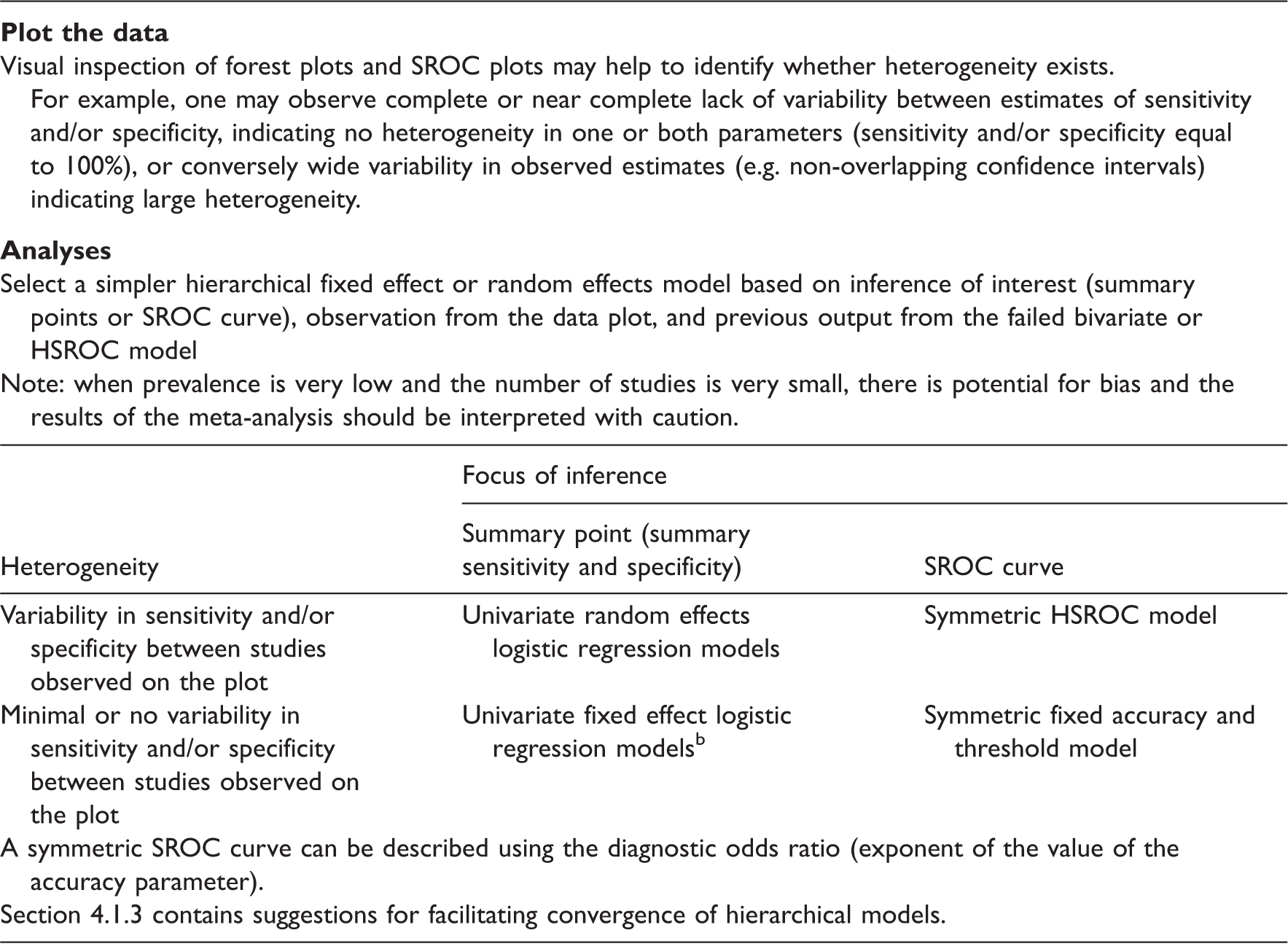
Bivariate or HSROC models either failed to converge or converged (i.e. met the convergence criterion) but gave unreliable estimates (e.g. with no standard errors, or dependent on starting values).
The symmetric fixed accuracy threshold model is equivalent to simultaneously fitting two univariate fixed effect logistic regression models for sensitivity and specificity.
Given the poor performance of simpler models like the fixed accuracy and fixed threshold models in the simulation, we urge meta-analysts to carefully explore their data and visually inspect forest plots and SROC plots before undertaking meta-analyses. Such preliminary analyses will provide an indication of the degree of heterogeneity and the pattern of scatter of the study points in ROC space. These analyses and the output from unstable or failed models should inform the approach for simplifying hierarchical models as shown by the appendicitis example. Although more complex and seldom used in practice, a Bayesian approach is an alternative to the maximum likelihood approach. In an empirical evaluation, both approaches were found to be similar although Bayesian methods suggested greater uncertainty (wide credible intervals) around the point estimates. 6
A normal distribution is typically assumed for the random effects in hierarchical meta-analytic models; violation of this assumption may contribute to non-convergence. Heavy tailed distributions such as t or Cauchy distributions may be used instead of a normal distribution,2,11 but random effects are restricted to be normally distributed in SAS NLMIXED and Stata. A Bayesian approach allows alternative distributions though a normal distribution is often assumed in practice. 21 As the models are often fitted using a maximum likelihood approach, our intention was to offer solutions within the hierarchical framework recommended for meta-analysis, using one of the software packages that have made meta-analysis of test accuracy studies more accessible to meta-analysts. A composite likelihood approach (implemented in R using the glmmML package) that offers some robustness to model misspecifications was recently proposed. 28 Results from the simulation study where the composite likelihood method and the bivariate generalized mixed model were applied to data generated from a bivariate t distribution suggested the methods were insensitive to the heavy tailed distribution under the logit link function. We used only the logit link in our models.
Our simulations and application to motivating examples support and extend empirical evidence suggesting that univariate methods generate summary results similar to those derived using full hierarchical methods.4,6,29 Our findings also agree with a recent simulation study evaluating the performance of the bivariate model. 30 However, our study is more comprehensive including application to real motivating examples, investigation of a broad array of possible models, suggestions for improving model convergence and guidance on how to select an appropriate model. Furthermore, we do not prescribe a limit on the number of studies required to fit a hierarchical model, rather the merit of applying a particular model should be carefully assessed as we have illustrated with our examples.
Our study has some limitations. First, we were not able to fully explore the effect of heterogeneity or varying the threshold. We addressed factors we considered vital, and varied the sample size of studies in a meta-analysis to reflect reality. According to Begg, 31 the statistical properties of hierarchical models are likely to be most vulnerable when the number of studies is small, and also when sample sizes are highly variable. Second, analyses of the simulated datasets were conducted only in SAS and convergence rates may differ between software packages because of differences in obtaining starting values and model fitting options. Nonetheless, SAS is the software most often used to fit HSROC models in frequentist analyses and we were able to explore several options for improving convergence. Third, when comparing models, we did not limit analyses to datasets that converged across all models. Non-convergence occurred more frequently in challenging datasets where poor model performance (bias, MSE and coverage) can be expected. Therefore, more complex methods with poor convergence rates may be biased or give imprecise estimates. The performance of simpler models with better convergence rates should also be affected but if the models give unbiased and precise estimates, then simpler models are robust and applicable in such situations.
In summary, random effects logistic models should be the default approach for test accuracy meta-analyses. We recommend UREMs for sensitivity and specificity if a bivariate model fails, or a symmetric HSROC model if estimation of a SROC curve is required and the HSROC model fails. If homogeneity can be assumed, the two models can be further simplified to their fixed effect equivalent. However, when prevalence is very low and the number of studies is very small, the results of any meta-analysis should be interpreted with caution.
Footnotes
Acknowledgements
We thank the two referees for their valuable comments which helped to improve this paper.
Declaration of conflicting interests
The author(s) declared no potential conflicts of interest with respect to the research, authorship, and/or publication of this article.
Funding
The author(s) disclosed receipt of the following financial support for the research, authorship, and/or publication of this article: This work was supported by the United Kingdom National Institute for Health Research [DRF-2011-04-135].