Sage Journals: Discover world-class research

Abstract

The study of electricity resource adequacy (i.e. quantifying the risk of future resource shortfall) typically uses standard metrics such as Loss of Load Expectation and Expected Energy Unserved. A range of possible risk model outputs are critiqued in this paper as a basis for decision analysis on capacity procurement, starting with the current standard approach (in which risk is commonly monetised as EEU multiplied by VOLL), and moving on to alternatives such as risk averse metrics and wider visualisations of risk profile. There are concerns in principle from a decision analytic perspective with using expected money as a utility function. Also, while there is interest in use of risk-averse metrics such as Conditional Value-at-Risk (CVaR), these might not capture all aspects of risk profile that are of interest. To obtain a comprehensive picture of the risk profile of a system, it is necessary to visualise a range of distributions of outcome measures, rather than using single number metrics. Providing such visualisations is likely not to provide the basis for a transparent risk standard, and options are discussed such as setting a level for a single metric that is occasionally revised according to changing profile of resources. Any such metric-based approach should also be supplemented by assessment of wider aspects of risk profile, for instance through examining distributions of outcome metrics. The inherent uncertainty, due to data limitations and imperfect representation of the system in the model, should also be acknowledged appropriately in estimation of such metrics.

Keywords

Resource adequacy risk aversion decision analysis decision support CVaR wind power

Introduction

Power system resource adequacy (RA) is the field of managing the risk that there will be insufficient supply resource to meet electricity demand. Studies vary as to the precise class of events in scope, but is generally taken to encompass the balance of resources without considering fine detail of system operation (see¹ for a survey of current issues). This remains a topic of great interest, due to the need to maintain an appropriate level of system reliability as the profile of resources evolves towards a lower carbon portfolio – and hence it is a key topic in assessing the performance of energy technologies within the system, and how technologies relevant to the net zero transition complement each other (or not) at whole power system level.

The area of RA also provides an excellent example of wider issues in project and policy appraisal, and in decision analysis, in that relevant decisions typically involve balancing capital investment costs (which are relatively concrete) against future reliability of the system (quantification of which is both more uncertain, and is not a cashflow that can immediately be incorporated in a monetised cost-benefit analysis).

RA studies typically use a standard set of risk metrics to quantify system reliability: Loss of Load Expectation (LOLE), the expected (in the statistical sense) duration of shortfall in the future year or season under study; Expected Energy Unserved (EEU), the expected volume of energy demand not supplied; or if going beyond these, further summary statistics such as System Average Interruption Duration/Frequency Index (SAIDI/SAIFI).² Formal decision analysis for capacity procurement tends to involve either a risk level target set with respect to one of these statistics, or a Cost-Benefit Analysis (CBA) in terms of a per-MWh Value of Lost Load (VOLL) multiplied by EEU^3,4 – historically less formally justified standards in terms of a deterministic measure of the margin of installed capacity over peak demand were common,¹ though these are now less widespread due to increased use of probabilistic analysis and the difficulty in including new technologies such as renewables without this.

There are issues in principle with the use of such summary statistics, which can have substantial practical consequences.

• Decision makers are likely to be risk averse, and interested in variability of outcome in individual years, as well as an average over possible outcomes. Expected value indices such as LOLE and EEU by definition do not reflect this, and thus decisions based on current decision analysis approaches might not properly reflect the concerns of decision makers.

• One single-number index cannot capture the whole risk profile of a system, and if the mix of supply and demand changes there may be changes in risk profile that these indices do not capture. There is nothing fundamentally wrong with the use of summary statistics, but they must be customised to and reflect the needs of decision makers.

• Standard approaches do not specify who the decision maker is. For instance, stakeholders (including ultimate decision makers in governments) tend to be very risk averse about electricity security of supply, due to the consequences for society and the economy if confidence in the electricity system decreases.

• The disruption costs of events are often assessed on a narrow basis of direct costs to customers, and not considering points such as wider societal and economic confidence in a robust electricity supply.

• It may not be natural to trade off investment and disconnection costs on the same (usually monetary) scale, that is they may not be commensurate⁵ (the formal decision analysis term for whether quantities can naturally be compared on the same numerical scale). For instance, many customers are unlikely to be indifferent between having supply and being paid monetary compensation, though this is implicitly assumed in many analyses.

Other works have looked for instance at use of multiple metrics,¹ inclusion of risk-averse metrics within optimization problems,⁶ and construction of probability distributions of ex post outcome metrics⁷ (and references therein, plus the Belgian standard references within an international comparison by Burke⁸). This paper, however, goes beyond previous literature through its critical discussion of how current practices reflect decision maker interests; and how decision making can be improved using a wider range of outputs available from standard risk model structures. For a general reference on relevant principles of decision analysis on which this work is based, including risk aversion, see⁹.

This paper will first describe and critique present approaches to adequacy assessment and capacity procurement in Section 2, before presenting in Section 3 alternatives such as risk-averse metrics and broader visualisations of risk profile to support decision makers. This is illustrated with results for Great Britain, considering a range of wind generation capacities. Section 4 provides an extended discussion of issues of application and relevance to wider decision appraisal, and finally Section 5 presents summary conclusions. A nomenclature of abbreviations is included as an Appendix.

Standard picture of decision analysis for capacity procurement

Risk modelling for resource adequacy

This section provides a brief overview of the resource adequacy modelling on which results are presented, based on a Great Britain (GB) system supplied by wind and conventional generation. This is satisfactory for our purpose of demonstrating use of model outputs in supporting decision making, where the key point is how a changing penetration of wind energy changes the overall risk profile. Issues of extension to other resources such as storage and interconnection to other systems, and uncertainty management arising from limited data on extremes and complexity of systems spanning multiple countries, will be discussed in Section 4.

We denote random variables with uppercase and constants with lowercase. X_t, Y_t and D_t denote available conventional and renewable generation, and demand, respectively at time t in the future period under study; then the surplus Z_t = X_t + Y_t − D_t. This section is consistent with standard references^2,10, but expressed in slightly different notation.

Non-sequential model

Let the period for which an assessment is being made (e.g. a future peak season) be divided into n hours. LOLE, the expected number of hourly shortfalls in the period is^I:

L O L E = E [\sum_{t = 1}^{n} I (Z_{t} < 0)] = \sum_{t = 1}^{n} P (Z_{t} < 0),

(1)

and the EEU is defined as:

E E U = E [\sum_{t = 1}^{n} \max {0, - Z_{t}}] .

(2)

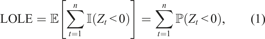
This is commonly referred to as a non-sequential model, as unless there are technologies such as storage which explicitly link the system states at different times, the terms in the sum may be evaluated separately, and the times re-ordered without affecting the result.

For statistical modelling, it is often more convenient to work in a time-collapsed picture with the time-collapsed variables Z, X, Y, D representing surplus, supply, and available demand, at a randomly chosen point in time. For a system that does not have storage or other technologies which link time periods, the LOLE is then specified as

L O L E = n P (Z < 0) = n P (X < D - Y),

(3)

and an analogous formula applies for EEU.

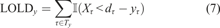
The most common means of estimating the distribution of D_t − Y_t is to use the empirical historic data directly in predictive risk calculations, sometimes referred to as hindcast.^2,11 The hindcast estimate of LOLE conditional on a particular historic weather year y is then

{L O L E}_{y} = \sum_{τ \in T_{y}} P (X_{τ} < d_{τ} - y_{τ})

(4)

where T_y is the set of times in historic year y, d_τ − y_τ is written in lower case as it is historic data rather than a random variable, and historic times are indexed by τ. LOLE conditional on no particular weather year is then usually estimated as LOLE = (1/n_Y)∑_yLOLE_y, where n_Y is the number of years of data (and similar for EEU). As discussed later, there can be substantial uncertainty in any estimate of unconditional risk level, as the estimate of the mean will often be dominated by a small proportion of the historic years.

Time sequential model

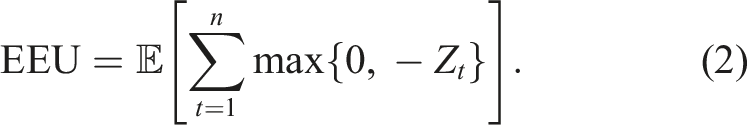
For model outputs beyond the standard expected value indices, such as the distribution of energy unserved, or the distribution of Loss of Load Duration (LOLD, the random variable of which LOLE is the mean) a time sequential model would be required. LOLD is specified as

L O L D = \sum_{t = 1}^{n} I (Z_{t} < 0),

(5)

and the energy unserved (EU) as

E U = \sum_{t = 1}^{n} \max {0, - Z_{t}} .

(6)

A wide range of other possible outputs may also be calculated, the usual mechanism for doing so being Monte Carlo simulation.

Stochastic process models must then be estimated for X_t and (D_t, Y_t). In practice, again a common way to proceed is to use a hindcast estimate for the process of demand and wind, that is

{L O L D}_{y} = \sum_{τ \in T_{y}} I (X_{τ} < d_{τ} - y_{τ})

(7)

and similar expression for EU. The aggregate available conventional capacity is usually specified as a sum of stochastic process models for each individual unit, with the unit models commonly (as here) being a two state Markov birth-death processes.

Decision analysis for capacity procurement

It is common to look at capacity procurement for a single future year, which for simplicity we will do here. This is the approach taken in the GB capacity market, where a target risk level is set based on a cost-benefit analysis (CBA) for the future year considered,¹² or might represent a long run equilibrium problem.¹³

The standard CBA can then be expressed as an optimization problem³:

m i n c (R) + [V O L L] \times [E E U] (R)

(8)

over the possible sets R of capacity-providing resources.³ The annualised procurement cost c and EEU are both functions of R. This is commonly simplified⁴ to

m i n [C O N E] \times r + [V O L L] \times {[E E U]}_{r},

(9)

assuming that the addition may be represented by a continuous real variable r, of which the procurement cost is a linear function, and the EEU is a decreasing function of r such that the optimization problem has a unique solution^II. Here Cost of New Entry (CONE) and VOLL take fixed values, and [EEU]_r is the expected energy unserved if the volume of capacity procured is r; it is straightforward to generalise this to non-constant CONE and VOLL.

In practice, this assumption implies that the addition should be small compared to the resource already present (generally the case in capacity markets, where the volume of new capacity is usually limited); and does not contain renewable generation or storage for which independence between existing and additional units does not apply.

Consequences of choice of VOLL

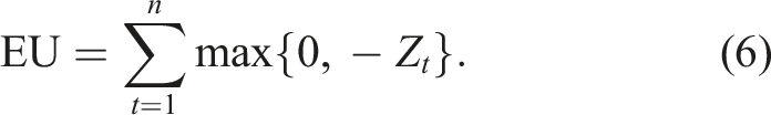
At the value of r which minimises (9),

{[L O L E]}_{r} = \frac{[C O N E]}{[V O L L]}

(10)

(A derivation of this result may be found in a previous paper by one of the present authors³). There are various challenges to taking this as an ‘optimal’ solution for the real world, even if EEU is regarded as a sufficient summary statistic of risk profile.

• Studies usually implicitly assume that the control room can disconnect the amount of load required and no more, with perfect foresight. This is not the case in practice, which implies an increase in energy unserved.

• An average VOLL across all customers is usually used, that is the interests of customers who are relatively indifferent to disconnection are treated interchangeably with interests of customers who are more averse to disconnection, even if there is no discrimination as to who is disconnected involuntarily. If one accepts the idea of monetising unserved energy using VOLL, should customers’ interests be averaged in this way, or should more weight placed on the interests of customers who are more inconvenienced by being disconnected?

• As in the introduction, one needs to consider whether reliability and procurement costs are commensurate, that is whether they can be compared on the same numerical scale.

This standard optimization picture in (9) typically recommends a level of reliability similar to the GB standard of 3 h/year LOLE, whereas a system that unreliable would probably be deemed politically unacceptable. For instance, in GB, a system margin warning can be a major news story,¹⁴ whereas this lowest level of system warning actually means that some hours ahead of real time the operator was not certain of having their usual real time operating headroom, that is nowhere near a shortfall in real time – if actual real time shortfalls happened in a substantial proportion of colder winters, the reaction in public debate would be stronger still.

Using a higher (not average) VOLL, based on the second bullet above, would push the reliability standard more towards a level that would be considered acceptable in this wider sense but would not consider wider issues of societal confidence in the electricity supply. Indeed if such factors beyond individual customer damage are considered important, then for use in comparing different capacity portfolios VOLL might be chosen such that (9) gives an acceptable level of system-level reliability, rather than being based on customer surveys. It is certainly the case that making different judgments associated with the first two bullets can change the ‘optimal’ level of reliability from (9) very substantially.

Beyond the conventional framework

Background and multicriteria formulation

Most formal decision analysis frameworks for capacity procurement assume the approach described in the previous section, i.e. monetising future reliability in terms of VOLL multiplied by expected energy unserved. Clearly capital costs are naturally in terms of money, though there may be uncertainty in the monetary sum, or one may wish to use a capacity price curve (i.e. as more is procured, the unit cost of capacity increases) rather than a fixed CONE – we have already discussed whether this can naturally be compared with reliability on the same numerical scale. Moreover, expected monetary return is rarely a utility function that reflects decision makers’ interests, particularly for mitigation of rare high impact events, and thus introducing a degree of risk aversion seems natural.

The simplest evolution of (9) would be to extend this framework to a multi-criteria decision question, seeking a Pareto frontier on which EEU cannot improved without disbenefit in terms of cost, and vice versa. However, for this case mapping the Pareto frontier is in fact equivalent to a sensitivity analysis on VOLL, so results for it are not presented here.

Data for examples

The following sections present results for an example based on the GB system. The standard approaches described previously are used for risk calculations. A comparison between scenarios of different installed wind capacities is made by using the same portfolio of available conventional capacity for each scenario; and for each scenario of installed wind capacity shifting the supply-demand balance to give a common EEU of 3 GWh/year, to give a controlled experiment for illustrative purposes^III. For instance, one might hypothesise that at higher penetrations of renewable generation, for a given value of standard indices such as LOLE or EEU, greater variability of supply leads to greater variability of outcome. This comparison is controlled in the sense that it looks at overall risk profile for a range of scenarios which have the same value of the headline EEU.

The scenario of installed conventional capacity is based on one originally provided by National Grid ESO, with a small random element added to each capacity due to the commercial sensitivity of the raw data. For sequential models, availability probabilities from NGESO are supplemented with mean repair time data from the IEEE Reliability Test System.¹⁵

GB demand data for the 12 peak (winter) seasons 2005-17 are used, with an estimate of historic available embedded renewable capacity added back on. Demand data are rescaled to a common system scenario according to historic values of the Average Cold Spell (ACS) Peak statistic, with the given scenario defined by an ACS value.

The wind generation data used are from Renewables Ninja¹⁶, and combine historic reanalysis wind speed data with a future scenario of what is connected to the system. Hourly capacity factors (CFs) for onshore and offshore wind in the ‘near term’ wind fleet from¹⁶ are used, and for a given scenario of onshore and offshore wind capacity connected to the system these hourly CFs are multiplied by the respective GW installed capacities and added to give a total hourly available capacity. The division between onshore and offshore for a given level of total installed wind capacity is based on projections described by Sanchez¹⁷.

Thus our example system is generally representative of the GB system and will suffice for our illustrative purpose, however for a fully applied GB study one would need to use data that are specialised to the particular decision question considered.

Risk averse metrics

Background

It is possible to define alternative single number metrics which give a measure of risk aversion, for example the well known (Conditional) Value at Risk (VaR and CVaR),¹⁸ with respect to model outputs such as the constructed distribution of energy unserved. This is defined as for a random variable U as

{[C V a R]}_{α} = E [U | U > u^{'}]

(11)

where P(U ≥ u′) = 1 − α for a risk threshold parameter α. Thus the mean of U is the special case [CVaR]₀, and if U is the energy unserved then CVaR is a generalisation of the standard EEU index – while one can use other mappings of EU and LOLD to give risk averse utility functions, this would not have the same attractive property of generalising the expected value indices.

CVaR has the further beneficial property of convexity when embedded in a wide range of optimization problems.¹⁸ We do note however that where it is not necessary to embed within an optimization model, there can be difficulties in communicating CVaR results outside the specialist community, particularly as for low degrees of risk aversion the risk threshold u′ will sit in the other tail of the distribution of U from the one of interest. Another diadvantage is that CVaR values with different α are not directly comparable, despite having the same dimensions.

Calculating risk-averse indices will in general require time-sequential modelling, as quantities such as EU and LOLD are functions of the full time series of surplus/deficit. The exception would be to work with VaR and CVaR with respect to the snapshot LOLP or Expected Power Unserved (i.e. the probability of a shortfall, or expected shortfall, at a randomly chosen point in time¹⁹). This would, however, need to be interpreted carefully. For instance, VAR with respect to snapshot LOLP may have a useful interpretation in terms of the expected number of hours with surplus below a given level, but other combinations of VAR/CVaR with LOLP or EPU might not be so interpretable.

Example

Figure 1 shows CVaR with respect to EU as a function of α, for a range of installed wind capacities. As in all examples, for a controlled experiment the scenarios of different installed wind capacity have the same EEU. As anticipated in the section on data, as the wind capacity increases, the CVaR for a given α also increases. This is consistent with a hypothesis that greater variability of supply would lead to greater variability of outcome – however the effect is not very large, and the next section will explore how CVaR as a summary statistic does not reveal the most striking change in the risk profile at higher wind capacities.

Figure 1.

CVaR as a function of the risk aversion parameter α for a range of installed wind capacities.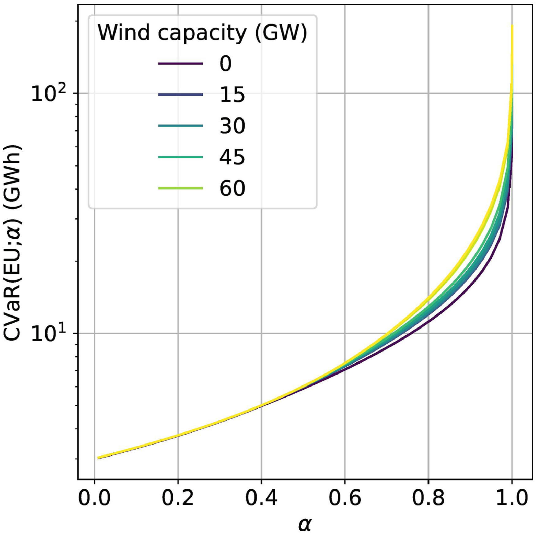

Visualisations for decision makers

Instead of attempting to define metrics in this way, one could instead provide visualisations to decision makers of the consequences of particular decisions in different scenarios of planning background, and let them decide on that basis how much capacity to procure. Even if there is still a preference of working with summary statistics for formal decision analysis, there is value in supplementing this with a wider range of visualisations to understand more broadly the system’s risk profile, or the consequences of results from formal optimization models.

This is an attractive idea in principle, though to go with such visualisations one needs the necessary skills in how to use them well – both on the part of the analysts in terms of how to create visualisations, and also in terms of how some technical statistical understanding on the part of decision makers may be necessary. On the other hand, visualisations such as these may be more tangible and easier to communicate than summary statistics such as CVaR. Appropriate use of scenarios and supporting narratives can help here, potentially using an interactive dashboard to provide model outputs and narratives of consequences for decisions under consideration.

Figure 2 provides an example of this for a scenario with fixed EEU of 3 GWh/year, and for a range of installed wind capacities. There is substantial variation with installed wind capacity of the distribution of EU in our experiment, but rather less variation in the distribution of LOLD. However while the former explains the variation of CVaR with respect to EU, the CVaR being a summary statistic of the distribution of EU, the difference between scenarios of different wind capacities is less striking in the CVaR results than in the underlying probability distribution.

Figure 2.

Scenario with fixed EEU = 3 GWh/year.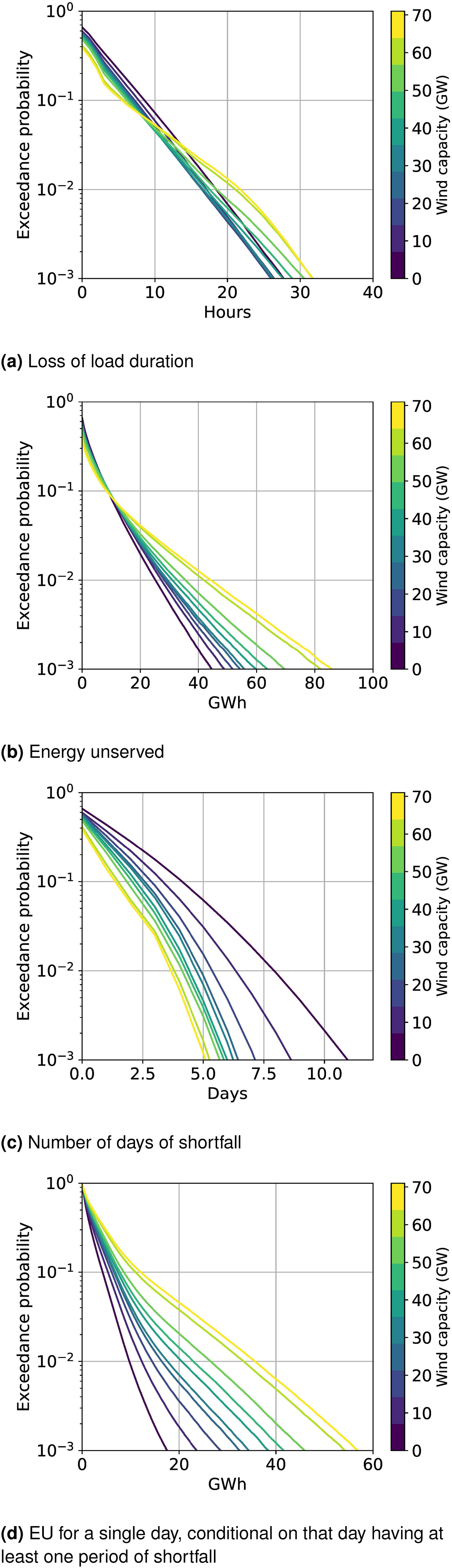

One can look further at the overall risk profile through the distributions of number of days with a shortfall, and of the probability distribution of EU within a day conditional on that day having a shortfall. It is clear from the lower two panels of Figure 2 that at higher wind penetration the same EEU is made up (in a probabilistic sense) of fewer days of greater shortfall. The variation with wind capacity of these two distributions is rather greater than that of the distributions of LOLD and EU – this difference may well be material for decision making, demonstrating how one might go in to considerable detail of risk model outputs to understand fully how the risk profile is changing.

There are important caveats on these results as quantitative calculations for the real GB system. We have carried out a calculation using a standard approach to illustrate important issues for decision support analysis in the model-world, but for a fully applied study one would need to specialise the statistical estimation to the relevant scenario, and to consider whether the modelling assumptions made give meaningful results on low probability events with respect to the real world.

Discussion

Statistical issues

In addition to this paper’s technical work exploring the range of model outputs available from standard calculations and how these might be used, there are also important statistical and uncertainty management issues which must be considered. These include estimation of model inputs, including having a limited number of examples in the historic record of extreme conditions, estimates of the availability properties of conventional generation at these times, and modelling of very complex continental-scale systems.

It is common in reliability analysis to have limited direct historic data on failure events, particularly in an area such as resource adequacy where there is a specific external driver of stress events (i.e. the weather). The consequent uncertainty in estimation of model outputs tends to increase in systems with high renewables penetrations, where the highest values of (demand minus renewables) are from times combining sufficiently high demand with low renewable resource – this tends to concentrate risk in a smaller number of events as compared to a system where risk is driven by the highest values of demand.

Strikingly, these conditions that drive risk at high renewable penetrations would not otherwise be regarded as extreme in any one location, where they would appear to be a standard and benign winter day with fairly low temperature and little wind. This dominance of risk profile by a limited number of years will manifest itself in different ways depending on the way the demand and renewable resource interact, and how much storage is connected to the system; for an example with a high storage penetration see²⁰.

This effect is illustrated for the example of this paper in Figure 3. At low penetrations of wind generation, 2005-6 does not make a substantial contribution to the calculated EEU, as peak demand was quite modest that winter. However, due to the very calm conditions on certain days of fairly high demand, at high wind penetrations this becomes the most significant winter by far in driving the outcome of the risk calculation.

Figure 3.

Proportion of estimated EEU arising from 2005-6 data.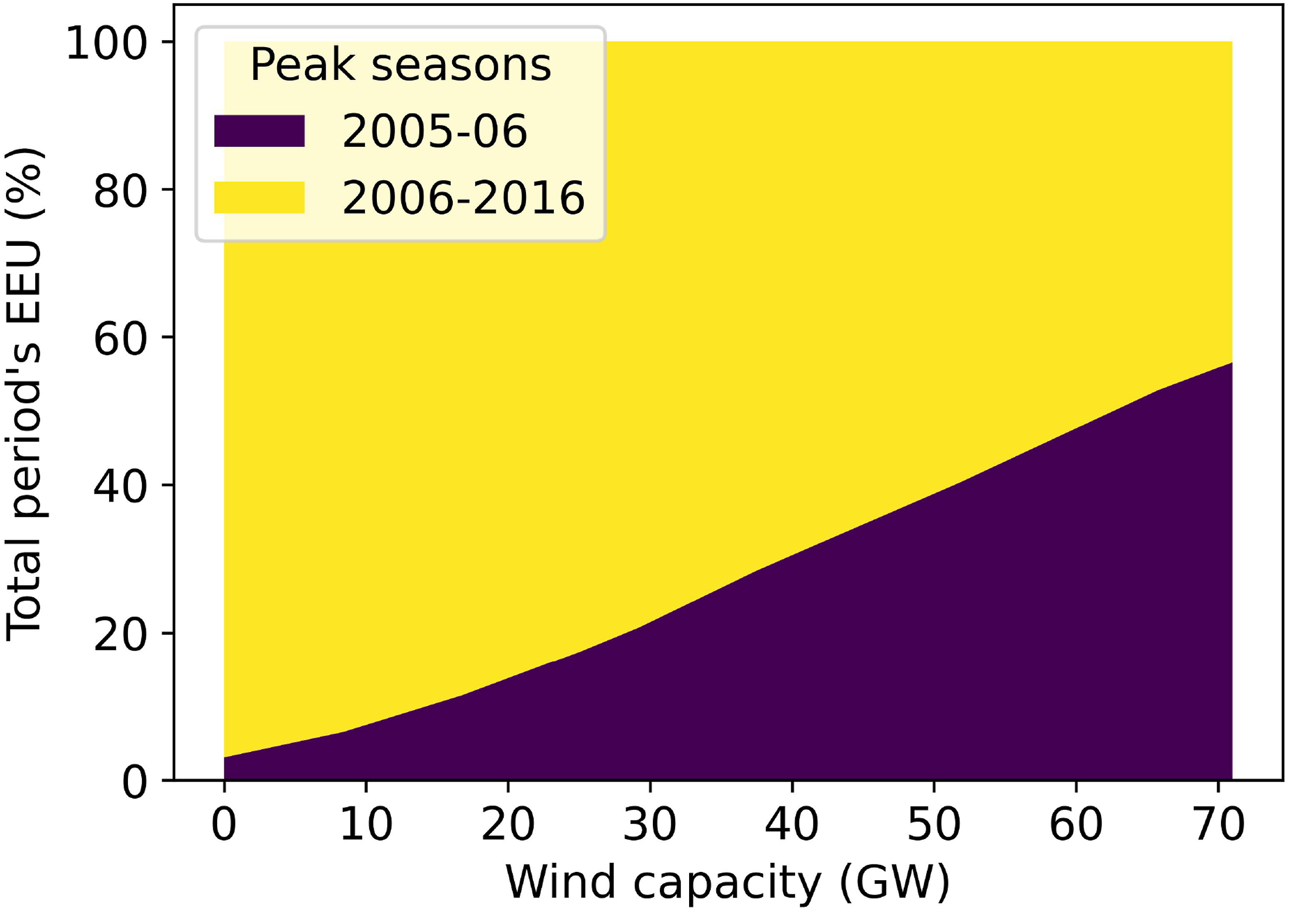

As a further illustration based on the experiment in this paper, Figure 4 presents the same analysis as Figure 2(b), except with the data from winter 2005-6 omitted^IV. At high wind penetrations, the estimated probability of very severe outcomes is then much lower than if data from that outlier winter are included.

Figure 4.

Probability distribution of Energy Unserved (same experiment as Figure 2(b) except that data from 2005-6 are omitted).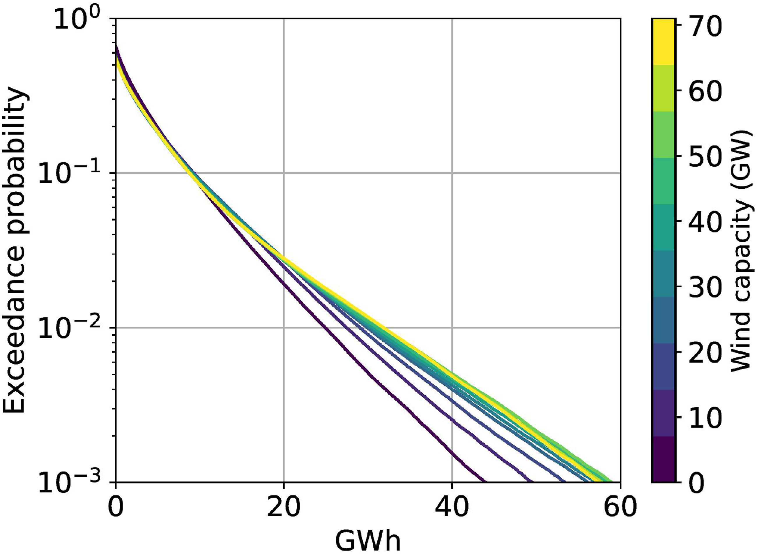

A particular manifestation of this will be in estimating tail event metrics such as VaR or CVaR of energy unserved with a high threshold - for instance in assessing what a one in n year outcome is. Even if one assumes that past weather is statistically representative of the relevant future year, by definition one will pick up a relevant weather year on average once every n years. Historic data will thus be very sparse, and estimates of such metrics (not conditional on particular weather) will be speculative.

Another key issue of uncertainty management is interconnection across very wide (continental scale) areas. As GB is an island system, this manifests as undersea connections to Ireland, Norway and the main continental European system. The level of interconnection between GB and other systems is forecast to rise rapidly; for instance one scenario study by the system operator has a minimum of 20 GW of connections to other systems on GB peak demand which is currently a little over 50 GW, making interconnector support a key consideration in evaluating adequacy risk.²¹ However there will be considerable uncertainty in any statistical characterisation of available support from other systems, due to the volume of model assumptions and data involved in continental scale assessments, and when carrying out a study knowledge of other systems almost certainly being poorer than knowledge of one’s own. The need to bring interconnection into assessments is recognised in other systems, as discussed in¹.

Decision support for capacity procurement

There is broad recognition that planning for system adequacy needs to recognise the changing needs of present and future systems with high renewable penetrations.¹ In particular, it is necessary to recognise that if the profile of supply and demand changes in a system, then it may be difficult to track this using a small set of single-number metrics – this paper has demonstrated by numerical experiment how this can be the case in a system with increasing penetration of renewable generation. Decision support approaches must both be transparent to the decision maker and not oversimplify the situation.

Historically, resource adequacy standards have tended to be set in terms of a single metric, usually a variant of LOLE – either the expected number of days on which there is a shortfall (the classic LOLE standard in N America being 0.1 days/year LOLE²²), or the expected number of hours of shortfall (e.g. the GB standard of 3 h/year LOLE; this metric is usually referred to in N America as Loss of Load Hours, LOLH, though in Europe is more commonly referred to as LOLE). The IEEE Resource Adequacy Working Group has provided a full discussion of variants of the LOLE metric.²³

There is thus a tension between the need to reflect the increasing complexity of patterns of supply and demand, and the natural desire to have simple, transparent criteria for use in supporting procurement decisions. The structure of working in this more complex environment would be simpler if there is a single ‘controlling mind’ (i.e. a point of decision making in a single organisation, maybe with the decision vested in a single individual) which is able to take judgments as to how to balance different aspects of risk profile in a decision on capacity procurement. In that case, standard approaches to uncertainty management and multi-criteria decision analysis could then be used to handle the issues described.

However when there is an industry and policy need for a clearly defined standard, one must seek appropriate compromises which reflect the changing nature of power systems and are sufficiently grounded in the relevant decision science; there is unlikely to be one definitive best approach here applicable in all situations. A further consideration is what actually can be estimated confidently – in particular, in many systems it may be possible to make confident estimates of risk profile conditional on a particular weather year and on a statistical characterisation of available support from interconnectors, these being the principal sources of uncertainty in risk model outputs.

One basis for a solution could therefore be to set a public facing risk target, for use in capacity procurement, conditional on a single given weather and interconnector scenario, or an assumption that the available time series data characterise fully the range of future possibilities that might be faced. This would allow performance of alternative resource portfolios to be compared, but it might be necessary to check against other possible interconnector or weather scenarios that the outcome is likely to be robust. It may further be necessary to adjust either the risk target or scenario choice from time to time, in order to maintain an appropriate level of risk as the portfolio of technologies develops. A related challenge is that supply capacity is not a simple additive commodity of the kind that is traded in standard auctions; a full discussion of the consequence of this may be found in³.

It may also be necessary to make some special consideration of very extreme situations. If it is deemed infeasible to assign probabilities to events which are too sparse in the historic record, then these might be treated through scenario analysis – however if this means that there is a probability model used for some classes of event, but the events which really matter are excluded from this model, there might be logical gap in the framework.

Another situation might be where weather beyond a certain degree of severity introduces distinct failure modes which are not seen at all in less extreme, but still severe, conditions, for instance those of Texas in 2021.²⁴ A further example is the severe cold and snow in GB in 1962-62,²⁵ which would bring very substantial changes in demand patterns over an extended period of months if it occurred again. Apart from any difficulties with assigning probabilities or mean return times, such conditions might require bespoke studies of effect of temperature and snowfall on demand and the power system, going well beyond the modelling that suffices for more normal circumstances.

Finally we note that the transparency of metrics and visualisations for decision makers is a significant issue. Standard indices such as LOLE and EEU are sometimes regarded outside the specialist modelling community as as being hard to understand, and inside that specialist community there is recognition of limits on the information that they contain. It is likely that non-specialists will find some additional metrics such as CVaR more difficult still to understand, so it is vital to take appropriate care in communicating the information that they contain. It may be, however, that visualisations of probability distributions are easier to communicate in that they contain all the information on estimated statistics of a particular quantity, though initially some might find the overt presentation of probability distributions intimidating.

Relation to wider issues of project and policy appraisal

The questions discussed in this paper should also be seen in the wider context of decision analysis and project appraisal. Indeed this area of resource adequacy and capacity procurement often provides a very good exemplar of wider issues, in that with a fairly simple system model (at least for a single power system area), it presents a range of subtle statistical issues.

The master guide for such analysis in the public and regulated sector in GB is the HM Treasury Green Book²⁶; while this is explicitly about appraisal and evaluation of policies and projects in central government, it is very influential on decision analysis in wider contexts. One key principle is that categories of assessment in an appraisal should be monetised if possible; if monetisation is not possible they should be quantified on a different scale, and if quantification is not possible they should be assessed qualitatively.

There is no dispute that RA risk is subject to quantification, albeit with significant caveats on whether confident estimates can be made without conditioning on assumptions about weather and interconnector support. However, as mentioned earlier in this article, monetising RA risk is much more doubtful – and the standard monetisation in terms of expected energy unserved multiplied by a (fixed, survey based, averaged over customers) per-MWh value of lost load, tends to recommend an unacceptably low level of reliability. In addition to this top-down argument, there are bottom-up arguments against averaging interests of all customers including that disconnections do not discriminate between customers with different interests.

One could go beyond the standard monetisation by making the VOLL dependent on the depth and length of shortfall, and more generally by eliciting decision maker judgments as to how the economic value should be considered; or by considering variability of economic damage about the mean. However, this still runs into problems with scope: does one only include direct economic damage? Or does one wish to include in decision analysis wider issues such as the need for wider economic and societal confidence in a reliable electricity supply? The latter is likely to be of interest to high level decision makers.

This in turn is a wider example of the issue in appraisals of managing imprecisely defined concepts such as social value, environmental capital and cultural value; energy security may be regarded as an example of the former. There will usually then be uncertainty arising from questions of scope, and of the way that any monetisation is conceptualised. This means that uncertainty in monetisations goes beyond considerations of input, parameter and modelling uncertainty to uncertainty in the conceptualisation (essentially that equally reasonable and expert people might come up with different broad approaches). The problems with bringing such disparate criteria together into a single number score has been noted previously in an energy context by Hammond and co-authors.^27,28 A very prominent example in the wider GB infrastructure sector is the business case underpinning the present HS2 high speed rail project, in which many factors are combined into a single monetary CBA.²⁹

Going back to the specific case of resource adequacy, consequence is clearly quantifiable, and relative economic consequence between different scenarios is likely also be quantifiable – but on the latter, questions of scope might mean that this is naturally a multicriteria comparison. The problem comes with the final step of bringing everything together into a single line item of money, when procurement costs and reliability are not fully commensurate. In this and a very wide range of case studies in other domains, we would recommend the following:

• If monetisation is used, it should come with a sufficiently broad quantification of uncertainty, including consequences of social value etc. being imprecisely defined quantities;

• In parallel with monetisation, a multicriteria analysis should be performed, recognising where quantities are not fully commensurate, that is they cannot naturally be brought together in the same line item of money;

• Visualisations such as a red-amber-green representation of the different options against the range of criteria may be very helpful in presentation to decision makers.

Conclusions

This paper has critically discussed a range of risk model outputs as a basis for decision analysis on capacity procurement, starting with the current standard approach (monetising risk as EEU multiplied by VOLL), and moving on to alternatives such as risk averse metrics and wider visualisations of risk profile. There are concerns in principle from a decision analytic perspective with using expected money as a utility function, and other practical issues include uncertainty in estimation of risk metrics or distributions of outcome, and whether metrics summarise sufficiently broadly the risk profile as relevant to the decision question under study.

There is natural interest in use of risk-averse metrics such as Conditional Value-at-Risk (CVaR). However these might not capture all aspects of risk profile that are of interest, for instance not distinguishing between situations where more/fewer days of less/more severe shortfall lead to the same distribution of outcome. To obtain a comprehensive picture of the risk profile of a system, it thus seems necessary to visualise a range of distributions of outcome measures, rather than using single number metrics.

However, as commented earlier, providing such visualisations is likely not to provide the basis for a transparent standard, or target risk level, which might be on the basis of a single metric with a set level that is occasionally revised according to changing profile of resources; or alternatively, as discussed in³⁰, having targets for different metrics all of which must be met. Any such metric-based approach should also be supplemented by assessment of wider aspects of risk profile, for instance through examining distributions of outcome metrics, to ensure that nothing significant is missed by reducing a complex situation to single numbers.

While technical aspects of uncertainty quantification are out of scope for this paper, it must be remembered that sufficient assessment of uncertainty in model-based (probabilistic) predictions must be made. This arises both from inevitably sparse data on rare severe conditions, and from modelling challenges such as assessing the contribution of interconnection to other systems on continental scale. It is also necessary to have a systematic means of combining broad uncertainty management with decision analysis; one possible framework is a Bayesian decision support system as described in³¹, and any alternative would require similar functionality for combining a wide range of uncertainties.

Footnotes

Acknowledgements

The authors acknowledge discussions with A. Dobbie, H. Wynn, S. Zachary, and members of the IEEE RAWG and the RA activities of ESIG, EPRI and G-PST. They also acknowledge meetings in which Colin Gibson and Andrew Wright provided advice about decision maker interests based on their industry experience. Author Chris Dent further expresses gratitude to the late Colin Gibson for exchanges throughout CD’s career in energy systems, from which he learned much about power system planning and operation.

Declaration of conflicting interests

The author(s) declared no potential conflicts of interest with respect to the research, authorship, and/or publication of this article.

Funding

The author(s) disclosed receipt of the following financial support for the research, authorship, and/or publication of this article: CJD, AS, JQS, ALW and XY from the Alan Turing Institute `Towards Turing 2.0' programme under EPSRC Grant EP/W037211/1; CJD, JQS and ALW from the Turing Fellow project ‘Managing Uncertainty in Government Modelling’; NS a PhD scholarship from the Mexican Conacyt funding council. CJD, JQS and ALW also acknowledge Turing Fellowships from the Turing Institute; and CJD and JQS would like to thank the Isaac Newton Institute for Mathematical Sciences for support and hospitality during the programme Mathematical and Statistical Foundations of Data Driven Engineering when work on this paper was undertaken (supported by EPSRC Grant Number EP/R014604/1), associated with which CJD was partially supported by a grant from the Simons Foundation. CJD further acknowledges a grant from the International Centre for Mathematical Sciences under its Knowledge Exchange Catalyst scheme to work with the Global Power System Transformation consortium.

ORCID iD

Chris J Dent

Notes

Appendix

References

Stenclik

Bloom

Cole

, et al. Quantifying risk in an uncertain future: the evolution of resource adequacy. IEEE Power Energy Mag 2021; 19(6): 29–36. DOI: 10.1109/MPE.2021.3104076.

Keane

Milligan

Dent

, et al. Capacity value of wind power. IEEE Trans Power Syst 2011; 26: 564–572. DOI: 10.1109/TPWRS.2010.2062543.

Zachary

Wilson

Dent

. The integration of variable generation and storage into electricity capacity markets. Energy J 2022; 43(4): 231–250.

ACER. Decision 23-2020: on the methodology for calculating VOLL, CONE, and the reliability standard. [Online] Available: https://extranet.acer.europa.eu/Official_documents/Acts_of_the_Agency/Pages/Individual-decision.aspx, 2020 (accessed 4 Feb 2023).

Self

. Nonsense on stilts: cost-benefit analysis and the roskill commission. Polit Q 1970; 41(3): 249–260.

da Costa

Thomé

Garcia

, et al. Reliability-constrained power system expansion planning: a stochastic risk-averse optimization approach. IEEE Trans Power Syst 2021; 36(1): 97–106. DOI: 10.1109/TPWRS.2020.3007974.

Sheehy

Edwards

Dent

, et al. Impact of high wind penetration on variability of unserved energy in power system adequacy. In International Conference on Probabilistic Methods Applied to Power Systems. Beijing, China: PMAPS, October 2016, 14, pp. 161–206. doi:10.1109/PMAPS.2016.7764199.

Burke

. GB security of supply – international study on standards and implementation. IEEE Resource Adequacy Working Group, 2016, Available at: https://cmte.ieee.org/pes-rawg/meetings/ (accessed 17 Aug 2023).

Smith

. Bayesian decision analysis. Cambridge: CUP, 2010.

10.

Singh

Jirutitijaroen

Mitra

. Electric power grid reliability evaluation models and methods. Hoboken: Wiley/IEEE, 2019.

11.

Wilson

Zachary

. Using extreme value theory for the estimation of risk metrics for capacity adequacy assessment. Pre-print, 2019. Available at: https://arxiv.org/abs/1907.13050.

12.

UK Government . Capacity market. [Online] Available: https://www.gov.uk/government/collections/electricity-market-reform-capacity-market (accessed 4 Feb 2023).

13.

Bothwell

Hobbs

. Crediting wind and solar renewables in electricity capacity markets: the effects of alternative definitions upon market efficiency. Energy J 2017; 38(SI1): 173–188.

14.

Davies

. National Grid makes urgent call for companies to reduce electricity usage. Guardian Newspaper 2015, Available at: https://www.theguardian.com/business/2015/nov/04/national-grid-issues-urgent-call-for-extra-power (accessed 21 Aug 2023).

15.

Grigg

Wong

Albrecht

, et al. The IEEE Reliability Test System-1996. A report prepared by the reliability test system task force of the application of probability methods subcommittee. IEEE Trans Power Syst. 1999; 14(3): 1010–1020.

16.

Pfenninger

Staffell

. Renewables ninja. Available at: https://www.renewables.ninja/ (2015, accessed 6 Nov 2022).

17.

Sanchez

. Power system adequacy: on two-area models and the capacity procurement decision process. PhD Thesis. University of Edinburgh, 2023. Available at: https://era.ed.ac.uk/handle/1842/39744.

18.

Rockafellar

Uryasev

. Optimization of conditional value-at-risk. J Risk 2000; 2: 21–41.

19.

Zachary

Dent

. Probability theory of capacity value of additional generation. Proc IMechE Pt O: J Risk and Reliability 2012; 226(1): 33–43.

20.

Zachary

. Scheduling and dimensioning of heterogeneous energy stores, with applications to future GB storage needs. Preprint available at: https://arxiv.org/abs/2112.00102 (2023, accessed 17 Aug 2023).

21.

National Grid ESO . Network options assessment for interconnectors. Available at: https://www.nationalgrideso.com/research-and-publications/network-options-assessment-noa/noa-interconnectors (2022, accessed 17 Aug 2023).

22.

Billinton

Chu

. Early history on the application of probability methods in the evaluation of generating capacity requirements. IEEE LOLEWG Presentation 2014, Available at: https://cmte.ieee.org/pes-rawg/meetings/ (accessed 18 Aug 2023).

23.

Stephen

Tindemans

Fazio

et al. Clarifying the interpretation and use of the LOLE resource adequacy metric. In 2022 International Conference on Probabilistic Methods Applied to Power Systems (PMAPS), Manchester, UK, 12-15 June 2022.

24.

University of

Texas at Austin. The timeline and events of the February 2021 Texas electric grid blackouts. Available at: https://energy.utexas.edu/research/ercot-blackout-2021 (2021, accessed 18 Aug 2023).

25.

Royal Meteorological Society . The Big Freeze of 1963: one of the coldest winters on record. Available at: https://www.rmets.org/metmatters/big-freeze-1963-one-coldest-winters-record (2013, accessed 18 Aug 2023).

26.

HM Treasury . The Green Book: appraisal and evaluation in central government. Available at: https://www.gov.uk/government/publications/the-green-book-appraisal-and-evaluation-in-central-governent/the-green-book-2020 (2022, accessed 17 Aug 2023).

27.

Allen

Hammond

Harajli

, et al. Integrated appraisal of micro-generators: methods and applications. Proceedings of the Institution of Civil Engineers - Energy 2008; 161(2): 73–86.

28.

Hammond

Jones

O’Grady

. Environmental life cycle assessment (LCA) of energy systems. In: Chou

Wei

Yan

(eds). Handbook of Clean Energy Systems. Sustainability of Energy Systems). Wiley, 2015, vol vol. 6, pp. 1–26.

29.

HS2 Ltd . Economic Case for HS2: updated appraisal of transport user benefits and wider economic benefits. Available at: https://assets.publishing.service.gov.uk/government/uploads/system/uploads/attachment_data/file/3650/hs2-economic-case-appraisal-update.pdf (2012, accessed 21 Aug 2023).

30.

Stenclik

. New resource adequacy criteria for the energy transition. Energy Systems Integration Group Technical Report 2024, Available at: https://www.esig.energy/new-resource-adequacy-criteria/ (accessed 19 August 2024).

31.

Volodina

Sonenberg

Smith

et al. Propagating uncertainty in a network of energy models. In International Conference on Probabilistic Methods Applied to Power Systems (PMAPS), Manchester, UK, 12-15 June 2022.

Resource adequacy and capacity Procurement: Metrics and decision support analysis

Abstract

Keywords

Introduction

Standard picture of decision analysis for capacity procurement

Risk modelling for resource adequacy

Non-sequential model

Time sequential model

Decision analysis for capacity procurement

Consequences of choice of VOLL

Beyond the conventional framework

Background and multicriteria formulation

Data for examples

Risk averse metrics

Background

Example

Visualisations for decision makers

Discussion

Statistical issues

Decision support for capacity procurement

Relation to wider issues of project and policy appraisal

Conclusions

Footnotes

Acknowledgements

Declaration of conflicting interests

Funding

ORCID iD

Notes

Appendix

References