Sage Journals: Discover world-class research

Abstract

Production engine pass-off testing is a compulsory technique adopted to ensure that each engine meets the required performance criteria before entering into service. Gas turbine performance analysis greatly supports this process and substantial economic benefits can be achieved if an effective and efficient analysis is attained. This paper presents the use of an integrated method to enable engine health assessment using real pass-off test data of production engines obtained over a year. The proposed method is based on a well-established diagnostic technique enhanced for a highly-complex problem of a three-spool turbofan engine. It makes use of a modified optimization algorithm for the evaluation of the overall engine performance in the presence of component degradation, as well as, sensor noise and bias. The developed method is validated using simulated data extracted from a representative adapted engine performance model. The results demonstrate that the method is successful for 82% of the fault scenarios considered. Next, the pass-off test data are analyzed in two stages. Initially, correlation and trend analyses are conducted using the available measurements to obtain diagnostic information from the raw data. Subsequently, the method is utilized to predict the condition of 264 production turbofan engines undergoing a compulsory pass-off test.

Keywords

Engine modelling/simulation engine performance engine testing gas turbine performance

Introduction

Background

In the recent years of aviation, modern turbofan engines have driven the majority of commercial aircraft. Consequently, their ability to perform effectively is considered to be of vital importance to assure engine cost-effectiveness, safety and reliability. Large civil turbofan engines require 3 to 7 years of design and development before entering service. After the initial phase and before delivering an engine to a customer, each production engine must undergo a specific acceptance test, also known as pass-off test.¹ Production pass-off testing is a technique adopted to assure that each engine meets the predefined performance criteria based on which an engine can be accepted or rejected by the customer. Amongst numerous performance criteria, the most important is the ability of the engine to produce a specific amount of thrust within operating limits and a guaranteed Specific Fuel Consumption (SFC), which determines the acceptability of an engine as well as the engine’s selling price.

During pass-off testing, specific parameters are measured at certain stations along the engine’s gas path.² The measured parameters are then compared with specific predefined limits, which determine whether the engine can be accepted or not. Production jet engines may show variabilities during these tests.³ The investigation and identification of the root causes of variability, which can correspond to genuine changes in components and/or measurement errors, require an efficient way to estimate and analyze the real engine performance. The goal of gas turbine diagnostic methods is the detection of the aforementioned phenomena and the accurate estimation of the real condition of the engine.

Gas turbine performance modeling and analysis

Gas turbine performance simulation is an important tool that assists the design and performance of gas turbine engines. Several simulation tools, such as the Rolls-Royce Aero-engine Performance (RRAP), Pratt and Whitney’s State of Art Performance Programming (SOAPP) and Turbomatch (Cranfield University), have been developed and are widely used for gas turbine performance simulation and analysis. The parameters used for engine modelling and analysis can be classified into those measured along the gas path and on the testbed, and performance parameters.² The simulation tools can run in two different modes for both modelling and analysis, known as synthesis and its inverse process, analysis mode.^4,5 The accurate determination of the overall performance when the simulations are running in analysis mode is far more challenging than the synthesis mode.⁵ The complexity of the analysis has been discussed thoroughly in Zedda and Singh² and Provost.⁶

The correct functioning of a gas turbine engine is a result of the effective performance of the gas path components. As the engine operates, individual engine parts and mainly aerodynamic components that perform at different environmental conditions and power settings, are susceptible to degradation. It is clear that, in the presence of a degraded component, the overall engine performance is affected.⁷ A review of different deterioration mechanisms is provided by Zaita et al.⁸ Correspondingly to the inevitable component deterioration, measurement instrumentation is also susceptible to degradation, which is associated with a reduction in measurement accuracy. Measurement uncertainty arises due to random errors and bias in the measurements and can have a major impact on the overall analysis.^1,9 The variability in pass-off tests can be a consequence of measurement uncertainty or deficient calibration, genuine changes in components due to variations in manufacturing processes for production engines, and component degradation for engines that have been overhauled.

Review of GPA techniques

A variety of methods for gas path analysis has been proposed and applied in academia and industry. The first techniques were introduced by Urban,¹⁰ who established a linear relationship between the performance and measured parameters. It is based on the fundamental assumption of the existence of linearity for small parameter deviations¹¹ and expressed as

Δ x = C^{- 1} Δ z

(1)

where

Δ z

is the measurement deviation vector,

Δ x

is the component parameter deviation vector and C the System Matrix. This formulation, which has been adopted by various tools in the industry,^12,13 is only for the special case where the number of sensors and unknown health parameters is identical. The adoption of a different formulation is essential for overdetermined and underdetermined estimation problems.¹⁴

Next, Escher¹⁵ proposed non-linear models for diagnostic purposes targeting to improve engine condition prediction accuracy. The formulation of the diagnostic exercise is still based on the minimization of an error function⁴ that allows the inclusion of systematic measurement errors and noise in the state vector. The simplest approach contains the minimization of an error with respect to a Least Squares (LS)¹¹ or a Weighted Least Squares (WLS) error function, first introduced by Doel.¹³

Kalman Filter (KF) first introduced by Kalman,¹⁶ is considered to be a generalization of the WLS approach in the context of diagnostics. Ganguli¹⁷ stated that the disadvantage of this method is the inevitable ‘smearing’ effects observed in the state vector. In order to tackle this phenomenon, a modified version of the KF was proposed by Provost.^6,18 This technique was adopted by Rolls-Royce in the diagnostic tool widely known as the Generalized Ground-based Monitoring System (COMPASS).¹² Additionally, KF allows diagnostics at transients in contrast to the previous methods. A detailed comparison of different diagnostic methods can be found in Mathioudakis and Kamboukos^11,19 and Li.²⁰

Scope of present work

Identifying at an early stage the trends of a given engine data set, entangled amongst the general scatter and noise, is very demanding. The main challenges are associated with the limited number of available measurements and the high levels of correlation between them. The redundancy between measured and performance parameters increases the complexity in the investigation of specific patterns and the evaluation of relationships amongst the data. This makes the discussed problem multi-dimensional.

In appreciation of the requirement for a cost-effective and accurate evaluation of the condition of the engine,¹⁴ this paper introduces a diagnostic method, capable of evaluating the condition of an engine based on typical pass-off measured data. It is based on the utilization of an engine performance model, capable of matching a set of measured parameters by adapting the component health parameters and by including a sensor biases matrix in the numerical formulation of the method. The present method can identify the root causes of variability and estimate the condition of the engine and instrumentation given a linear System Matrix which relates health parameters and sensor biases to measured outputs and a measurement vector as an input. This is achieved via a well-established diagnostic formulation appropriately modified for the highly-complex problem of a three-spool turbofan engine.

The main advantages of this method are first, its capability to assess the performance of the engine and measurement instrumentation using a limited number of measurements and second, that the model does not require a priori data to be trained. This is achieved by enhancing a well-established optimization approach with a least-absolute error objective function, the ‘Concentrator’, which enables the potential to focus on a limited number of components.

The effectiveness of the method is demonstrated in a set of different simulated test cases; test cases containing only component faults, only sensor faults and a combination of component and sensor faults. Next, the integrated methodology is applied towards the analysis of a set of real test data obtained over a year from approximately 300 production three-spool engines, undergoing a compulsory pass-off test.

Methodology

Engine performance simulation

The diagnostic method presented here relies on the existence of an engine performance model. The engine model is developed using Turbomatch,²¹ developed by Cranfield University. It is designed based on a modular design concept, capable of simulating different engine configurations.

The performance of the whole engine is evaluated by solving mass and energy balance between the various engine components expressed via discrete component map characteristics. The code solves a system of non-linear equations using a Newton Raphson (NR) method. The engine model configuration used in this study is based on a modern three-spool high by-pass ratio turbofan design. The engine model has simulated the fan using two different components with separate characteristics representing the core (root) and the fan tip respectively.

Measurements and health indices selection

Engines undergoing pass off testing in ground test facilities typically measure the rotational speed of each spool, thrust, airflow, fuel flow as well as total and static pressures and temperatures at specific locations of the engine. The component parameters indicating engine performance cannot be measured directly and hence, are determined based on the discussed measurements.

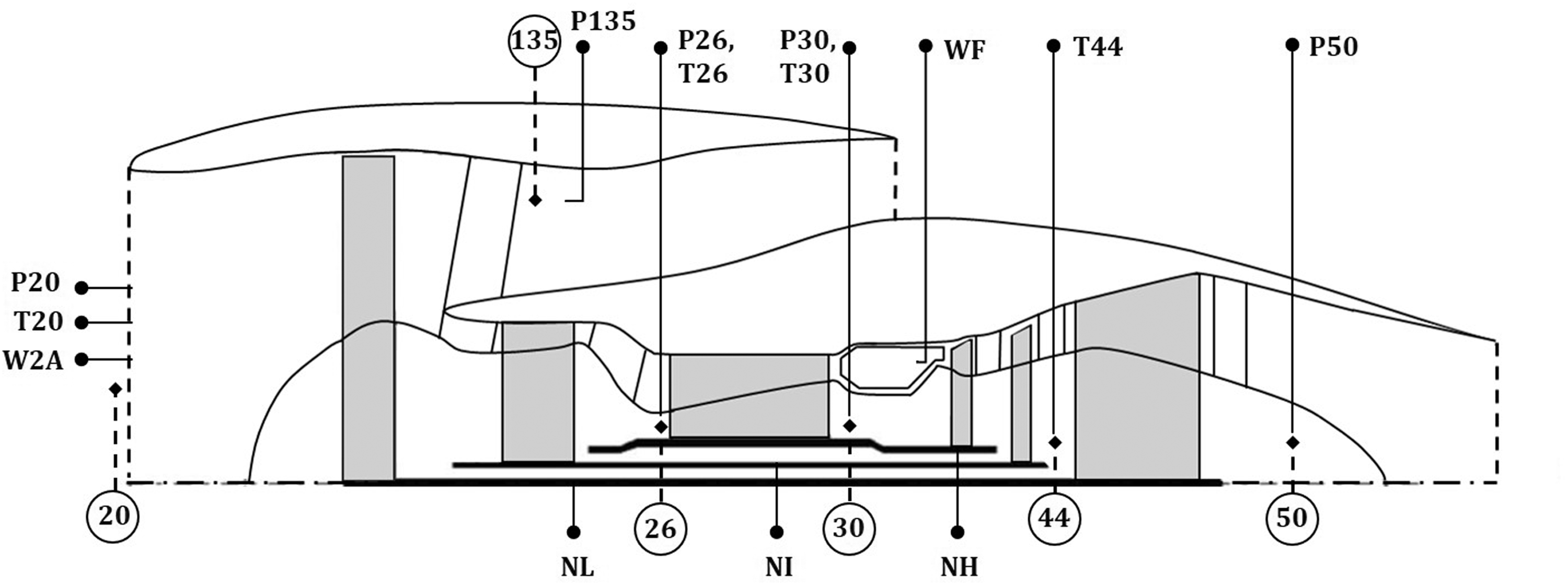
For the turbofan engine considered in the present work, the engine stations and available measurement are illustrated in Figure 1. Table 1(a) and (b) presents the available measurements; gas path measurements and operating conditions during pass-off testing. The Net Thrust ( $F_{N}$ ) is a power setting parameter, which is constant for all the engines during the pass-off test. Table 1(c) outlines the performance parameters capable of reflecting hardware changes. The parameters annotated with an asterisk (*) are directly measured during this test. The rest of the parameters are evaluated using an engine performance model running in analysis mode.

Figure 1.

Pass-off available measurements and station numbering (generic image inspired from GasTurb engine schematics).

Table 1.

Total pass-off test parameters (measured and calculated).

(a) Measured parameters			(b) Ambient and operating conditions			(c) Calculated parameters
No.	Parameters	Notation	No.	Parameters	Notation	No.	Parameters	Notation
1*	Fan Tip Exit Total Pressure	$P 135$	1*	Ambient Temperature	$T 0$	1	Fan Tip Efficiency	$η_{FAN, TIP}$
2*	HPC Entry Total Pressure	$P 26$	2*	Ambient Pressure	$P 0$	2	Fan Tip Capacity	$Γ_{FAN, TIP}$
3*	HPC Entry Total Temperature	$T 26$	3*	Relative Humidity	$RH 0$	3	IPC Efficiency	$η_{IPC}$
4*	HPC Exit Total Pressure	$P 30$	4*	Fuel Heating Value	$FHV$	4	IPC Capacity	$Γ_{IPC}$
5*	HPC Exit Total Temperature	$T 30$	5	Net Thrust	$F_{N}$	5	HPC Efficiency	$η_{HPC}$
6*	LPT Inlet Total Temperature	$TGT$				6	HPC Capacity	$Γ_{HPC}$
7	LPT Exit Total Pressure	$P 50$				7	HPT Efficiency	$η_{HPT}$
8*	Engine Inlet Airflow	$W 2 A$				8	HPT Capacity	$Γ_{HPT}$
9*	Engine Fuel Flow	$WFE$				9	IPT Efficiency	$η_{IPT}$
10*	LP Shaft Rotational Speed	$NL$				10	IPT Capacity	$Γ_{IPT}$
11*	IP Shaft Rotational Speed	$NI$				11	LPT Efficiency	$η_{LPT}$
12*	HP Shaft Rotational Speed	$NH$				12	LPT Capacity	$Γ_{LPT}$

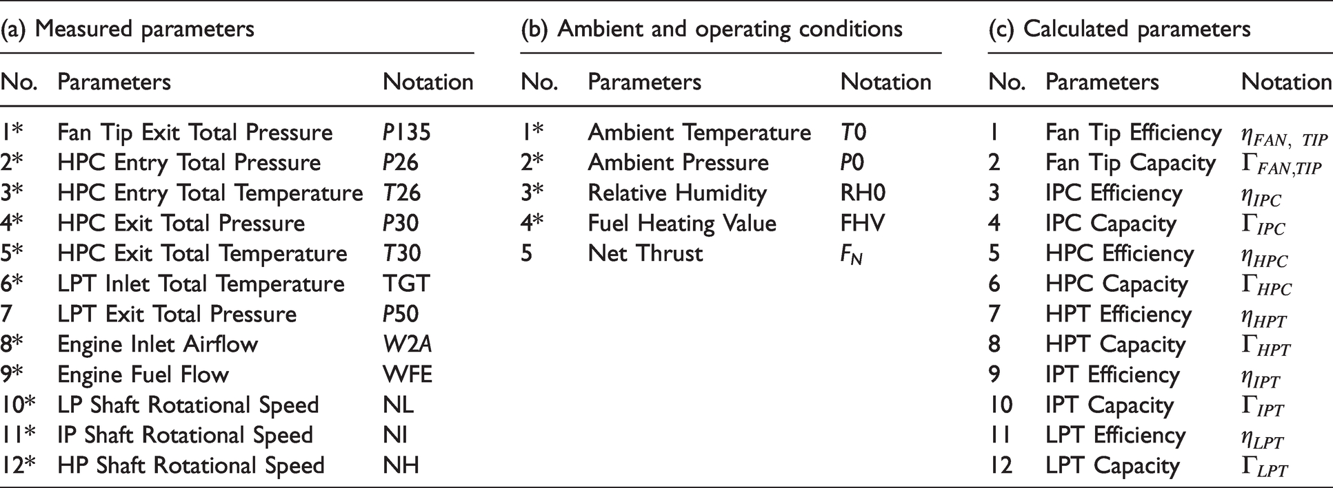
The available measurements are first corrected to standard ambient and operating conditions.¹ They are then expressed as a deviation from a reference engine, corresponding to the engine at nominal conditions. A key driver to the successful evaluation of the condition of the engine is the selection of a cost-effective set of measurements that can provide the maximum possible information. Several studies have been reported in the literature where different techniques are used for optimal measurement selection.^22,23 The present measurement subset is considered representative for today’s turbofan engines undergoing a pass-off test and hence, will be used as a reference subset in this paper. Table 1(a) and (b) presents a standard set of measured data during pass-off testing.

Diagnostic method

Formulation of diagnostic method

The proposed diagnostic method aims to evaluate the condition of the engine and measurement instrumentation, represented with a deviation vector of performance parameters $Δ x$ , based on a given set of measurements $Δ z$ , expressed as deltas, by formulating an optimization problem. The method accounts for both component changes and sensor biases and is based on the fundamental relationship

Δ z = C Δ x + v

(2)

where

Δ z

is a column vector

(m x 1)

of the measured parameters in a deviation form, C the System Matrix

(m x n)

Δ x

a column vector

(n x 1)

including the performance parameters in a deviation form and v is a column vector

(m x 1)

of noise included in the measured parameters.

The System Matrix C is extracted by conducting a sensitivity analysis using the representative engine model in Turbomatch.²¹ The sensitivity of the dependent parameters is evaluated by applying small changes in the independent parameters. A change of 1% in every parameter is selected in the present analysis. The generation of C is based on the assumption of existing linearity between the dependent and independent parameters – an assumption valid for a narrow range of performance deviation of $\pm$ 3%.¹ The resulting changes are then expressed as a deviation from a reference engine ( $Δ z = \frac{Z - Z_{Ref}}{Z_{Ref}} \cdot 100$ %). The matrix C comprises three independent matrices; component exchange rates (Table 1(c)), environmental exchange rates (Table 1(b)) and identity matrix resembling the sensor biases (Table 1(a)) and is represented as a two-dimensional Jacobian matrix. The resulting System Matrix C is presented in Appendix 2.

The available measurements m are limited in such tests and hence, the number of the performance parameters and sensor biases n will be greater than the number of the measured parameters (n > m). Specifically, there are n = 27 including component changes and sensor biases and m = 11 available measurements. As a result, the proposed system is under-determined.²⁴ Subsequently, an infinite number of solutions can be obtained for the vector $Δ \hat{x}$ and hence, an optimization technique is adopted to solve

Δ \hat{z} = C Δ \hat{x}

(3)

$Δ \hat{x}$ the state vector including component changes and sensor biases (Table 1(a) and (b)) and $Δ \hat{z}$ the estimated measurement deviation vector.

Selection of objective function

The discussed estimation technique is based on minimizing an error function, expressed in a form of a deviation of the estimated measurements and the input measurement vector

ϵ = | Δ z - Δ \hat{z} |

(4)

The domain comprises 11 equations – measurements and 27 unknowns – performance parameters and sensor biases. A Single-Objective (SO) optimization technique is adopted in this work. Specifically, the built-in MATLAB fmincon function is selected.²⁵ The selected interior-point algorithm is based on minimizing a multivariable function subjected to various constraints, as outlined in equation (5)

minimize f (x) subject to lb \leq x \leq ub

(5)

where

f

is the selected objective function and lb and ub are the lower and upper bounds, respectively.

Performance parameters are appropriately bounded (lb,ub), based on engineering judgment and prior knowledge regarding the expected variation in pass-off testing. A range of $\pm$ 3% is selected for this work. This is due to the fact that the current methodology is based on the assumption of a linear relationship between measured and calculated parameters for the range of [-3%, +3%].¹ Additionally, the highest recorded deviation during the pass-off testing is +3%. The present research investigates two different objective functions.

The first objective function that was selected is based on a least-squares minimization (L2-norm) and it is defined as

minimize f_{1} = \sum_{i = 1}^{m} {[\frac{Δ {\hat{z}}_{i} - Δ z_{i}}{Δ z_{i}}]}^{2}

(6)

The second objective function that was considered is a least absolute function (L1-norm) and it is defined as

minimize f_{2} = \sum_{i = 1}^{m} |\frac{Δ {\hat{z}}_{i} - Δ z_{i}}{Δ z_{i}}|

(7)

where

Δ \hat{z}

the predicted measurement vector and

Δ z

the measurement vector used as an input.

‘Concentrator’

A disadvantage observed when using the proposed method is that the estimated state vector $Δ \hat{x}$ included only non-zero coefficients. This tendency of the technique to ‘smear’ the variability in all the potential effects may result in an overestimation of the irrelevant or negligible changes. It can also result in an underestimation of dominant faults of components and sensors that may be overwhelmed due to this effect, also reported in.⁴

In order to overcome this limitation, Provost^6,18 presented an enhancement to the KF estimator, the so-called ‘Concentrator’. On the basis of this method,⁶ an alternative approach of this method is presented in this work.

It aims to guide the state vector to a limited number of component changes and sensor biases, corresponding to the dominant effects producing the observed variability. This is done by detecting the insignificant effects and removing them from the problem while maintaining the most relevant ones in the optimization process. This methodology is outlined in Figure 2 and is based on an iterative optimization procedure. The diagnostic method uses a measurement deviation vector recorded during pass-off testing as an input (11 measurements) and a System Matrix C extracted using a representative engine model (27 state variables). The iterative process is outlined below.

Figure 2.

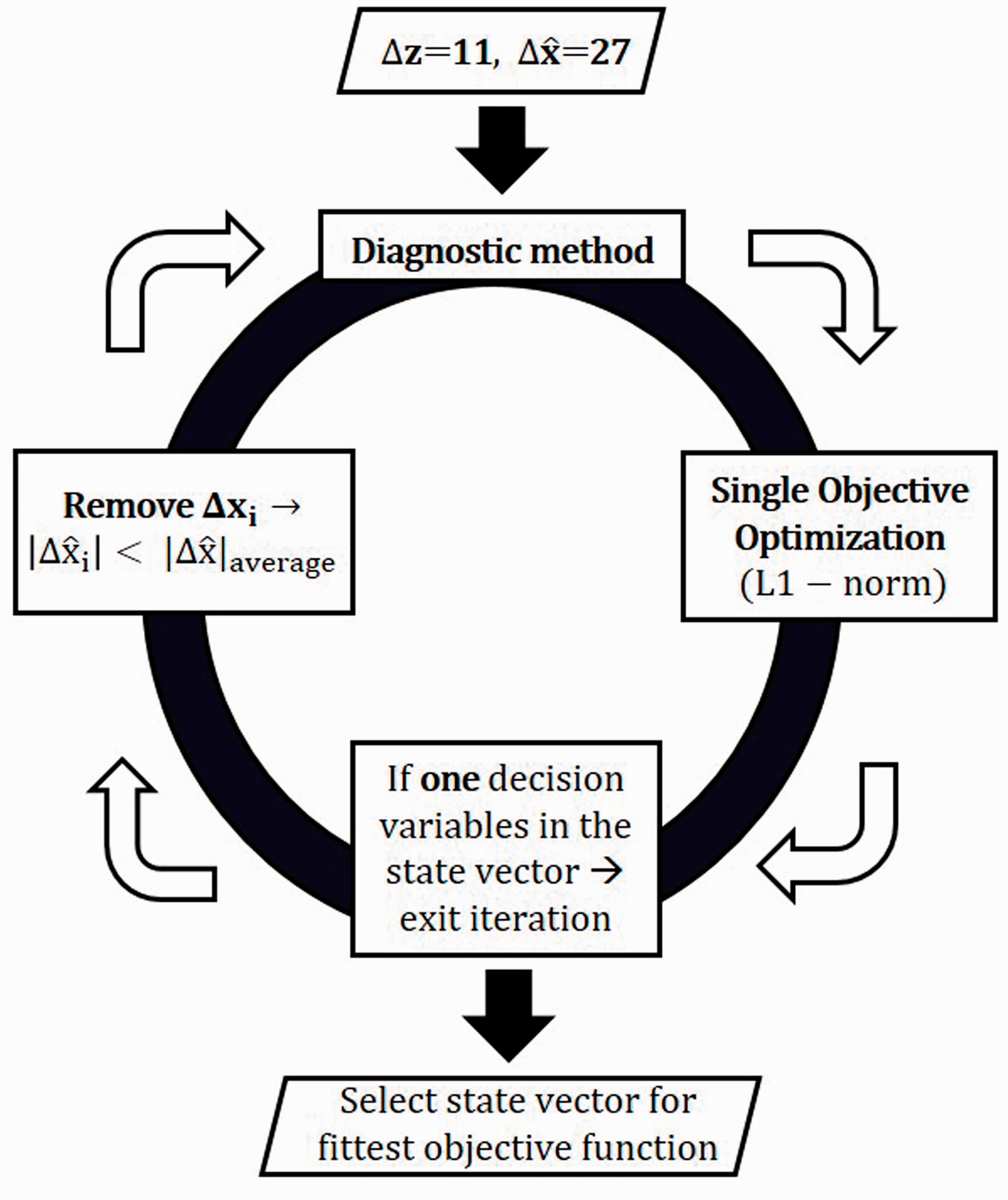
Schematic representation of the diagnostic process.

The optimizer initially runs with all the parameters, bounded with a [-3%; +3%]. Subsequently, the resulting state vector $Δ \hat{x}$ will contain 27 non-zero coefficients.

The objective function (L1-norm) is evaluated.

The absolute value of all the parameters in the state vector $Δ \hat{x}$ is calculated and sorted in descending order.

In order to start the ‘Concentrator’, the calculated coefficients are classified into two groups representing the ‘highest’ and ‘lowest’ coefficients. As ‘highest’ we refer to coefficients greater than the average value in the obtained state vector $(| Δ {\hat{x}}_{i} | \geq {| Δ \hat{x} |}_{average}$ ), which are kept in the optimizer. On the other hand, the ‘lowest’ coefficients corresponding to $|Δ {\hat{x}}_{i}| < {| Δ \hat{x} |}_{average}$ are removed from the optimizer by setting their boundaries to zero.

The optimizer re-runs with the parameters that have been selected in Step 4. A new state vector $Δ \hat{x}$ and hence, the corresponding value of the objective function is calculated.

The process continues iteratively until only one parameter remains in the model.

At each iteration, a different structure of the estimated fault parameters is constructed based on Step 4. The best structure is selected by comparing the values of the objective functions evaluated at each iteration. Thus, the state vector $Δ \hat{x}$ corresponding to the minimum objective function is the optimal structure of estimated fault parameters.

The obtained answer will go through a final modification. The elements in the best answer $Δ \hat{x}$ that are below a predefined value ( $\pm$ 0.5%) are excluded from the solution. This is done in order to result in a final estimate $Δ \hat{x}$ that includes only the dominant component changes and/or sensor biases.

Validation

The proposed estimation techniques; the SO algorithm and the modified version of the ‘Concentrator’ originally developed by Provost,⁶ have to be validated before applying them to the real engine data. The representative engine model is used in order to generate a population of different scenarios that are able to reproduce the effect of engine component and sensor faults.

The engine model first runs at Design Point (DP), representing the ‘reference’ engine. The fault scenarios are generated by applying one or more component degradations and re-running the model with respect to a predefined value of degradation. This is done by altering the efficiency and capacity scaling factors of the main turbo-machinery components. The measured parameters (Table 1(a)) are then extracted from the model, corrected for environmental conditions and expressed as a deviation $Δ z$ from the reference engine (DP simulation). In order to simulate sensor biases, one or more errors in the form of a percentage change are applied to the resulting measurement deviation vector. Noise is added to the simulated cases with a standard deviation approach for each one of the measurements.

Single-component changes and sensor biases are simulated first in order to compare the two objective functions considered. This is done by altering only one factor in each simulation. The magnitude of the simulated changes is selected to be +1% and -1%. The single-component changes and sensor biases are equal to the number of elements in the state vector (n = 27). Thus, the total number of single simulated changes is 54 (both +1% and −1%).

Next, it has been demonstrated that the complexity of the gas turbine engine together with the measurement uncertainty may lead to multiple component changes and sensor biases occurring simultaneously.¹ For this reason, pairs of component changes and sensor biases are simulated. It is clear that the number of available combinations is relatively high. Specifically, the number of pairwise combinations for a + 1% change in each effect is equal to 351 $((\begin{matrix} 27 \\ 2 \end{matrix}) = \frac{27!}{2! (27 - 2)!} = 351)$ .

Before proceeding to the evaluation of the effectiveness of the method, an example of a single component change is presented to illustrate the performance of the method. Table 2 outlines a typical output of the diagnostic method, for an indicative case of a + 1% change in the fan capacity with the rest of the parameters remaining unchanged. The output of the method is a state vector $(Δ \hat{x})$ , comprising all the possible component, environmental changes and sensor biases (1st column). Columns (a-d) represent the output of the diagnostic method for the two objective functions L2-norm ( $f_{1}$ ), L1-norm ( $f_{2}$ ) (Section “Selection of objective function”) when the ‘Concentrator’ is deactivated and activated respectively.

Table 2.

Typical diagnostic output in %.

$Δ \hat{x}$	Fault scenario	Diagnostic output
		SO L1-norm	SO L2-norm	Concentrator L1-norm	Concentrator L2-norm
		(a)	(b)	(c)	(d)
* $Γ_{FAN}$	1.0	0.4	0.18	1.0	1.0
$η_{FAN}$	0	−0.11	−0.14	0	0
$Γ_{IPC}$	0	−0.01	−0.01	0	0
$η_{IPC}$	0	−0.04	−0.05	0	0
$Γ_{HPC}$	0	0.01	0.01	0	0
$η_{HPC}$	0	−0.01	−0.01	0	0
$Γ_{HPT}$	0	−0.01	−0.05	0	0
$η_{HPT}$	0	−0.01	0	0	0
$Γ_{IPT}$	0	0	0	0	0
$η_{IPT}$	0	−0.03	−0.04	0	0
$Γ_{LPT}$	0	0.03	0.04	0	0
$η_{LPT}$	0	−0.11	−0.14	0	0
$T 0$	0	0	0	0	0
$P 0$	0	−0.01	−0.04	0	0
$F_{N}$	0	0.02	−0.03	0	0
P135	0	−0.01	−0.02	0	0
P26	0	−0.01	0	0	0
T26	0	0	0.01	0	0
P30	0	0.01	0.03	0	0
T30	0	−0.01	0	0	0
TGT	0	−0.03	0.02	0	0
P50	0	−0.01	0	0	0
W2A	0	−0.02	−0.01	0	0
WFE	0	0.19	0.1	0	0
NL	0	−0.19	−0.25	0	0
NI	0	0.02	0.05	0	0
NH	0	0.02	0.04	0	0

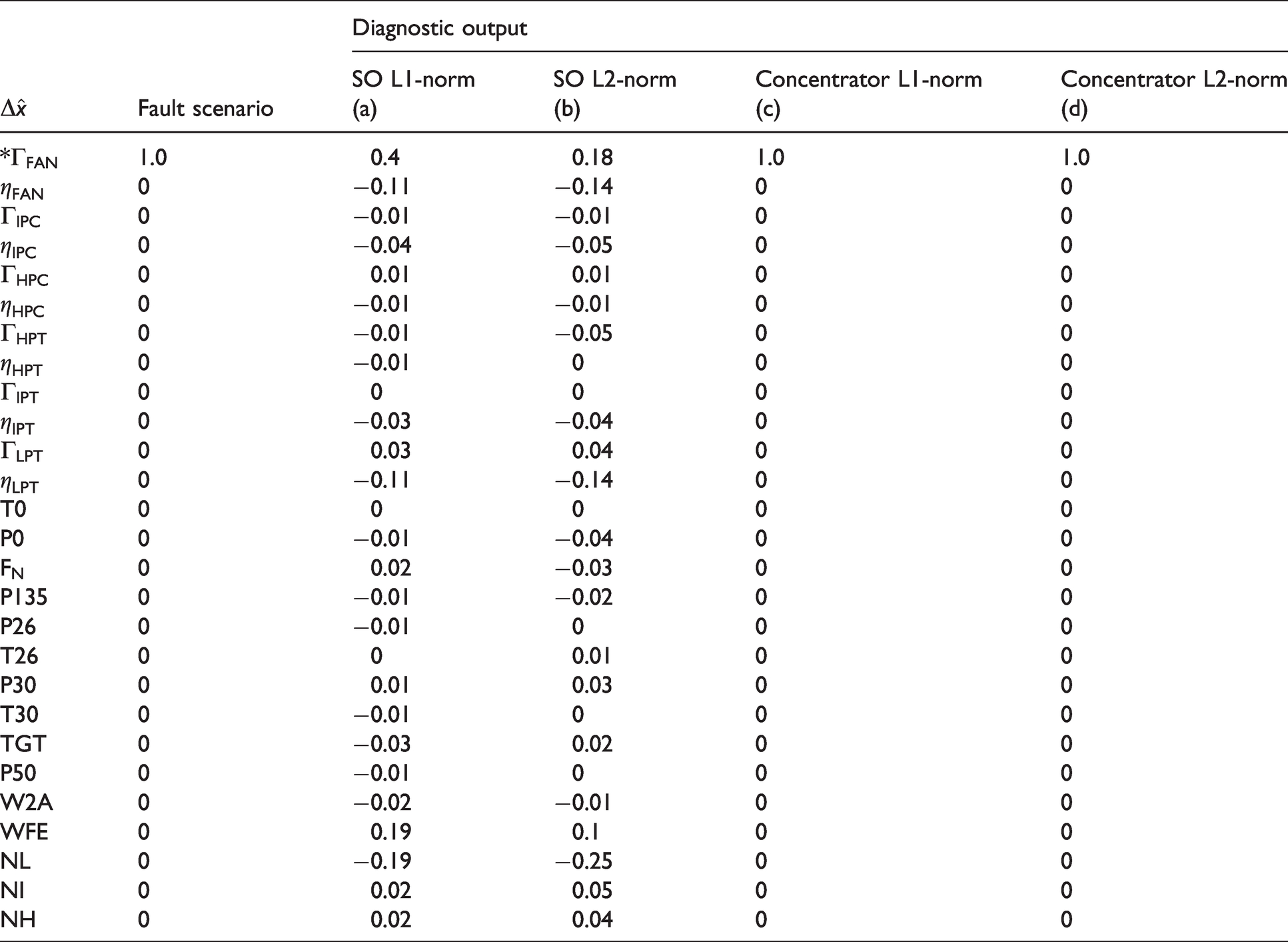
The utilization of the L1-norm objective function (a) estimates a 0.4% fan capacity while the rest of the parameters in the state vector remain less than 0.2%. The method is not able to predict the magnitude of the fault, as the predicted value is far from +1%. On the other hand, the L2-norm (b) objective function predicts a fan capacity of 0.18%. Moreover, the NL bias estimate produced by the L2-norm is larger than the estimate produced for the true parameter shifted (fan capacity). Specifically, the NL bias estimated is -0.25%. This indicates that the method is incapable of locating the fault and estimating the correct magnitude. This phenomenon is also reported in Stephen.²⁶ For both objective functions considered, the state vector includes non-zero parameters as both norms tend to spread the effect of a single component change to all the parameters in the state vector (‘smearing’ effect). It is noted, however, that this phenomenon is more obvious for the L2-norm function. When the ‘Concentrator’ is activated, the discussed ‘smearing’ effect is eliminated, and the method predicts a change of 0.92% and 0.82% for the L1-norm and L2-norm objective function, respectively (Columns c, d). At the same time, the rest of the parameters in the state vector are zero.

Simulated case: Single component changes and sensor biases – Comparison of L1 and L2

In this section, the two selected objective functions are compared. For simplicity purposes, only single component changes and sensor biases are presented.

Table 3 outlines 27 different fault scenarios and the predictions for them when the ‘Concentrator’ is deactivated. Each row of the table corresponds to a different simulated scenario. When the ‘Concentrator’ is deactivated almost all the parameters in the state vector are non-zero. In order to avoid very large tables, Table 3 presents only the parameter that changes in each simulation while the rest of the parameters in the state vector are not printed. A third column referred to as the ‘Other Change’ is added and corresponds to parameters in the state vector that are greater than the estimated change of the parameter subject to the fault change. For instance, for a simulated change of +1.0% in fan capacity ${(Γ}_{FAN}),$ if another parameter appears higher in the state vector, this parameters will be noted as ‘Other Change’ and this will indicate that the fault scenario is not observable.

Table 3.

L1-norm and L2-norm SO algorithm comparison: Estimated state vector by varying health parameters and sensor biases by 1% independently expressed in %.

$Δ \hat{x}$	Fault scenario	Diagnostic output
		SO L1-norm	SO L2-norm	Other change L1-norm	Other change L2-norm
		(a)	(b)	(c)	(d)
$Γ_{FAN}$	1.0	0.4	0.18	None	NL
$η_{FAN}$	1.0	0.23	0.23	None	$η_{LPT}$
$Γ_{IPC}$	1.0	0.22	0.16	NI	NI
$η_{IPC}$	1.0	0.24	0.21	None	None
$Γ_{HPC}$	1.0	0.31	0.26	None	None
$η_{HPC}$	1.0	0.22	0.22	$Γ_{HPC}$	$Γ_{HPC}$
$Γ_{HPT}$	1.0	0.7	0.44	None	None
$η_{HPT}$	1.0	0.37	0.3	None	None
$Γ_{IPT}$	1.0	0.48	0.4	None	None
$η_{IPT}$	1.0	0.39	0.28	None	None
$Γ_{LPT}$	1.0	0.29	0.26	None	None
$η_{LPT}$	1.0	0.24	0.25	$Γ_{FAN}$	$Γ_{FAN}$
$T 0$	1.0	0.29	0.55	None	NL
$P 0$	1.0	0.81	0.7	None	None
$F_{N}$	1.0	0.31	0.26	None	None
P135	1.0	0.7	0.58	None	None
P26	1.0	0.45	0.35	None	$Γ_{HPT}$
T26	1.0	0.66	0.58	None	None
P30	1.0	0.58	0.52	None	None
T30	1.0	0.76	0.7	None	None
TGT	1.0	0.75	0.75	None	None
P50	1.0	0.46	0.34	None	None
W2A	1.0	0.66	0.64	None	None
WFE	1.0	0.71	0.63	None	None
NL	1.0	0.69	0.62	None	None
NI	1.0	0.4	0.18	None	None
NH	1.0	0.23	0.23	None	None

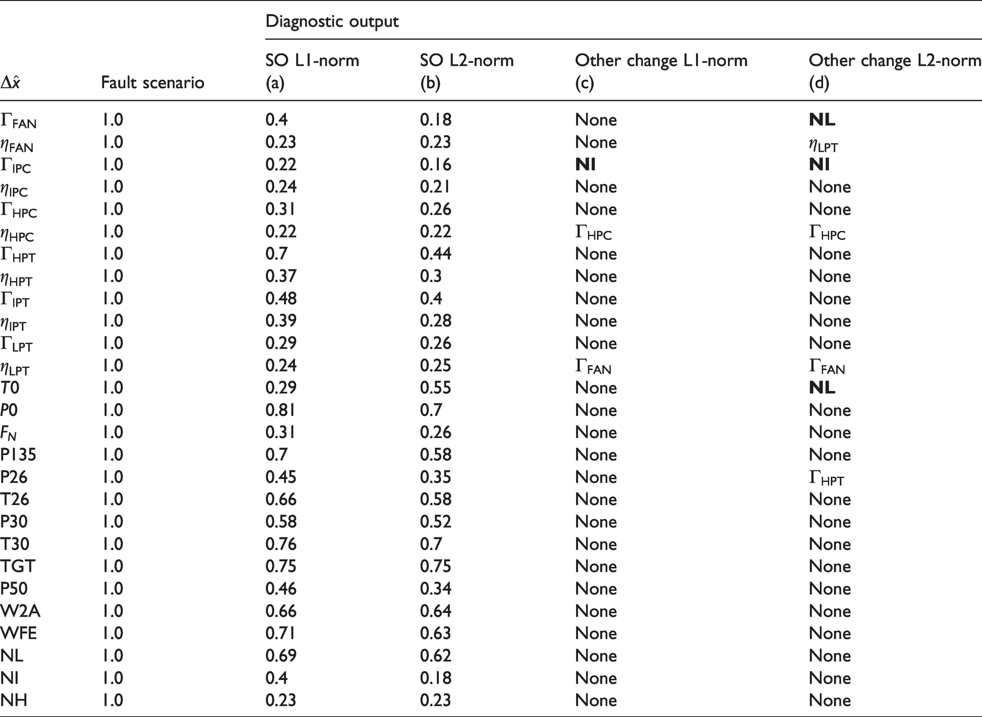
The predictions using the L1-norm are closer to the simulated magnitude compared to the L2-norm. Additionally, when using the L2-norm the system becomes less observable. This is explained by the fact that in 30% of the simulated cases, the faulty components are overwhelmed by others. As a result, the L2-norm is unable to capture the simulated changes and hence, it is concluded that the L1-norm is superior.

The same fault scenarios are examined with the ‘Concentrator’ activated. The L1-norm objective function is used for both the SO approach and the enhancement of the algorithm with the ‘Concentrator’.

Figure 3 illustrates a comparison between the optimization algorithms. Single Objective (SO) and Concentrator correspond to the diagnostic model when the ‘Concentrator’ is deactivated and activated, respectively. The results are presented as a percentage deviation from the reference engine operating in nominal conditions. It is observed that the predictions that were diverging from the applied fault (+1%) in Table 3, have now reached the optimum value for the health parameters (Figure 3(a)). On the other hand, it can be seen in Figure 3(b) that the sensor biases are less observable. This can be explained by the fact that the simulated change is small and hence, it can be easily overwhelmed by the noise added to the simulated data. It is noted, however, that the root-mean-square (RMS) error relative to the simulated fault scenarios for the sensor biases is estimated at 0.0175 and hence, the predictions from the diagnostic model are considered adequate.

Figure 3.

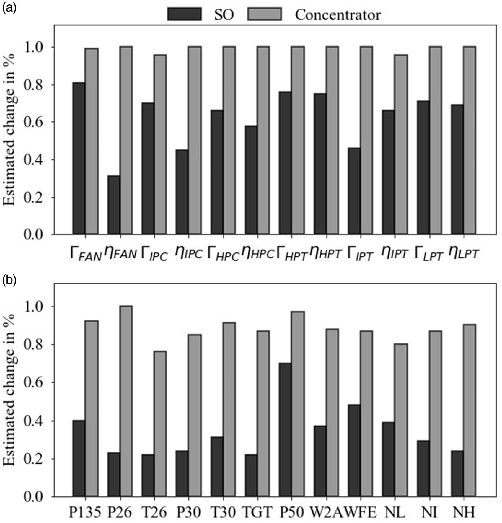
Comparison of the estimated (a) health parameters and (b) sensor biases of the L1-norm SO algorithm with the ‘Concentrator’.

Simulated case: Pairs of component changes and/or sensor biases

Having selected the most suitable objective function (L1-norm), the effectiveness of the tool is investigated for simulated combinations of component changes and sensor biases. For this demonstration, component changes and sensor biases were simulated in pairs. Specifically, 66 pairs of component changes and 156 pairs of both component changes and sensor biases were simulated. The magnitude of the simulated change is +1% for both parameters in the pair. Of the 222 pairs of simulated changes, the ‘Concentrator’ successfully detected 174 (78.4%). As successful detection, we refer to its capability of distinguishing the ‘faulty’ components or sensors while simultaneously matching the magnitude of the simulated change. The remaining 48 pairs (21.6%) are characterized as a ‘failure’ in the diagnostic process. With the term ‘failure’ we refer to two failure categories. The first one is that the analysis fails to locate the faulty components and hence, the calculated component changes and sensor biases differ from the simulated ones. The second one is that despite the fact that the faulty components are correctly located, there are significant differences in the magnitudes of the analyzed changes of one or both parameters of the pair compared to the simulated ones. Additionally, the same analysis was done using the L2-norm. The failure rate, in this case, is 29.6%.

The pairs of component changes were more difficult to analyze. Specifically, of the 66 pairs of component changes 39 pairs were successfully identified. The combinations of pairs of component changes are calculated based on $(\begin{matrix} Component Parameters \\ 2 \end{matrix}) = (\begin{matrix} 12 \\ 2 \end{matrix}) = 66$ .

On the contrary, pairs that consist of one simulated component change and one simulated sensor bias are more observable. Specifically, out of the 156 pairs, the analysis successfully detected 135 (86.5%). This demonstration was repeated for the 156 pairs of component changes and sensor biases using different signs; component changes are simulated with +1% and sensor biases with -1%. Out of the 156 pairs of simulated changes, the analysis successfully detected 135 (86.5%). The key conclusion regarding the validation of the diagnostic method is that out of the 405 simulated changes, 333 (82%) simulated changes were successfully detected. The same simulated changes are almost undetectable without the ‘Concentrator’. As a result, the 82% success in detection of the faulty components indicates that the performance of the tool is acceptable. For this reason, the analysis can be now used to examine the root causes of variability in the real pass-off test data.

Application of the method to real engine pass-off test data

This section examines a given set of available pass-off test data and uses the developed diagnostic method to evaluate the condition of the engines and identify the root causes of variability observed in the data. Figure 4 presents the SFC variation for the data set considered. It is observed that the SFC engine-to-engine variation may be significant with respect to the pass-off test predefined limits.

Figure 4.

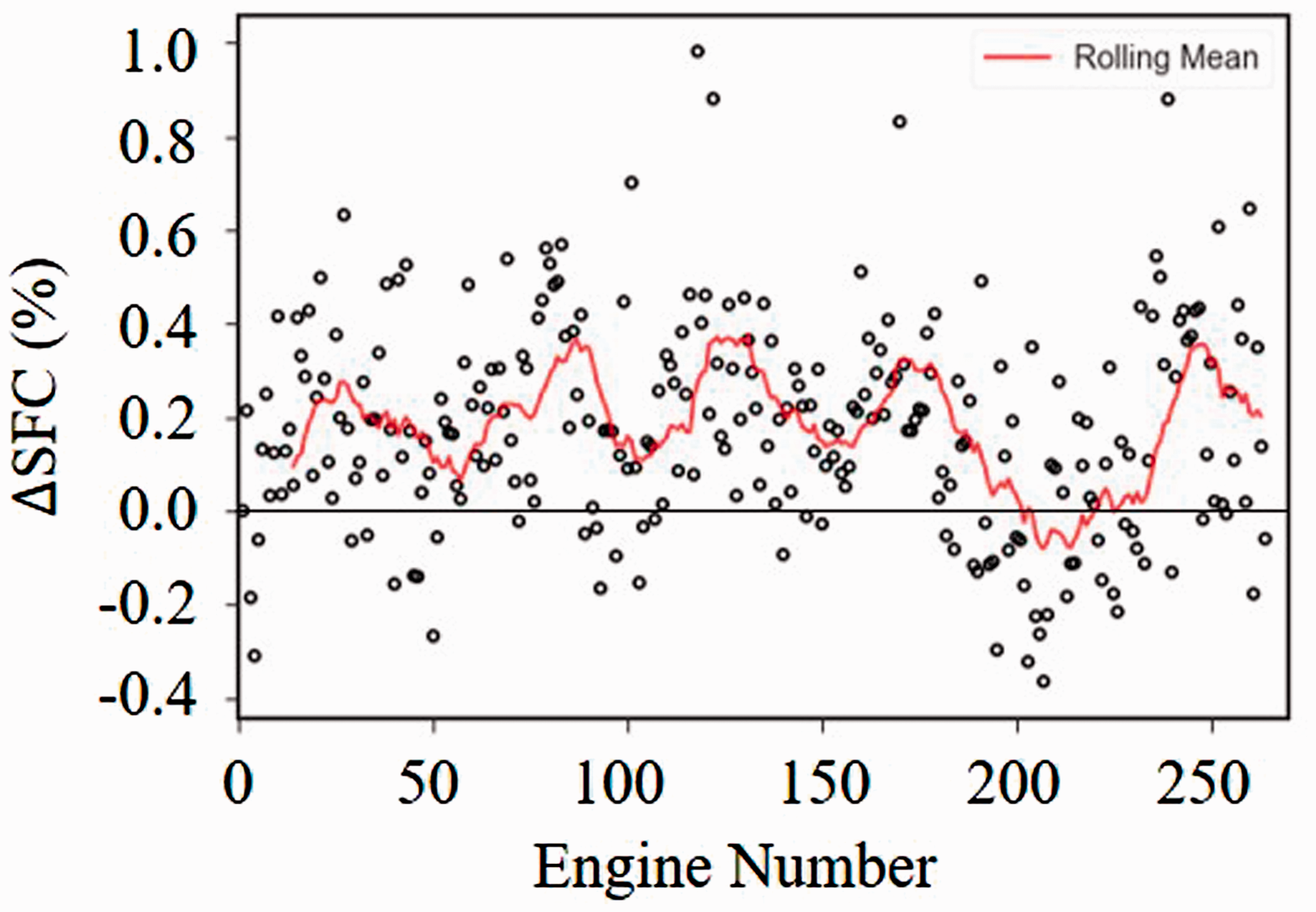
ΔSFC over engine number.

The observed variabilities are not critical to the pass-off process. However, understanding the behaviour of the engine population is considered to be of vital importance. The observed variability can be a direct outcome of, among others, genuine changes in components, caused by variations in the manufacturing process, or component degradation, or measurement noise and biases which propagate in the performance calculations.

The main factors generating noise are associated with weather conditions (humidity, wind, rain, and fog), atmospheric pollution, stabilization times and running history. It is therefore realized that the accurate performance analysis is difficult to be achieved due to the simultaneous presence of the aforementioned effects. First, the available measurements are corrected for the inlet conditions and are expressed as a deviation from a reference engine to reduce the variation in the raw data.

Pass-off real test data analysis

Initially, the simpler approach is to use the available data, measured and calculated parameters to conduct a correlation and trend analysis in order to get a better understanding of the inter-relationships between the data. Correlation analysis aims to evaluate the level of correlation between two variables x and y. The degree of correlation between the two variables is represented by a specific correlation coefficient, also known as the Pearson coefficient. The Pearson coefficient is defined as the ratio of the covariance of two variables (x, y) to sx and sy, the standard deviations of x and y, respectively (equation (8))

rx, y = \frac{Cov (X, Y)}{sx sy}

(8)

This equation can be applied to all the pairs in the available data. The output of this process is a symmetric matrix comprising the level of all the possible pairwise correlations. The obtained coefficients can range from −1 to +1. Off-diagonal correlation coefficients greater than 0.7 need to be examined.⁴ The pass-off test data correlations are outlined in Table 4, where only the lower triangular is printed.

Table 4.

Pearson correlation matrix for pass-off test data.

	NH	NI	NL	P135	P26	P30	P50	SFC	T26	T30	WFE	W2A	$η_{FAN, TIP}$	$η_{IPC}$	$η_{HPC}$	$η_{HPT}$	$η_{IPT}$	$η_{LPT}$
NH	1
NI	0.13	1
NL	−0.08	0.02	1
P135	0.01	0.13	0.24	1
P26	−0.68	−0.01	0.01	−0.01	1
P30	0.65	0.11	−0.14	−0.03	−0.2	1
P50	−0.24	0.1	0.19	−0.02	0.21	−0.36	1
SFC	−0.34	0.01	0.17	0.21	0.35	−0.32	0.05	1
T26	−0.19	0.02	−0.15	−0.07	0.38	0.09	−0.1	0.28	1
T30	0.53	0.15	−0.18	0.04	−0.09	0.72	−0.32	0.08	0.27	1
WFE	−0.34	0.01	0.17	0.21	0.34	−0.31	0.04	1	0.29	0.08	1
W2A	0.3	−0.01	−0.01	0.27	−0.13	0.47	−0.66	0.13	0.1	0.47	0.14	1
$η_{FAN, TIP}$	−0.25	0.04	0.23	0.85	0.03	−0.4	0.2	0.15	−0.16	−0.31	0.15	0.06	1
$η_{IPC}$	−0.23	−0.02	0.16	0.07	0.25	−0.21	0.24	−0.07	−0.8	−0.32	−0.07	−0.18	0.18	1
$η_{HPC}$	0.08	−0.04	−0.07	−0.1	−0.24	0.05	−0.12	−0.08	0.66	−0.14	−0.08	0.02	−0.12	−0.85	1
$η_{HPT}$	0.66	0.11	0.03	0.02	−0.46	0.62	−0.2	−0.37	−0.62	0.52	−0.37	0.29	−0.18	0.36	−0.54	1
$η_{IPT}$	0.1	0.03	−0.15	−0.17	0.19	0.46	−0.17	−0.09	0.86	0.38	−0.08	0.18	−0.33	−0.78	0.69	−0.29	1
$η_{LPT}$	0.51	0.1	0.47	0.04	−0.26	0.69	−0.09	−0.53	−0.17	0.29	−0.52	0.23	−0.17	0.01	0.03	0.58	0.23	1

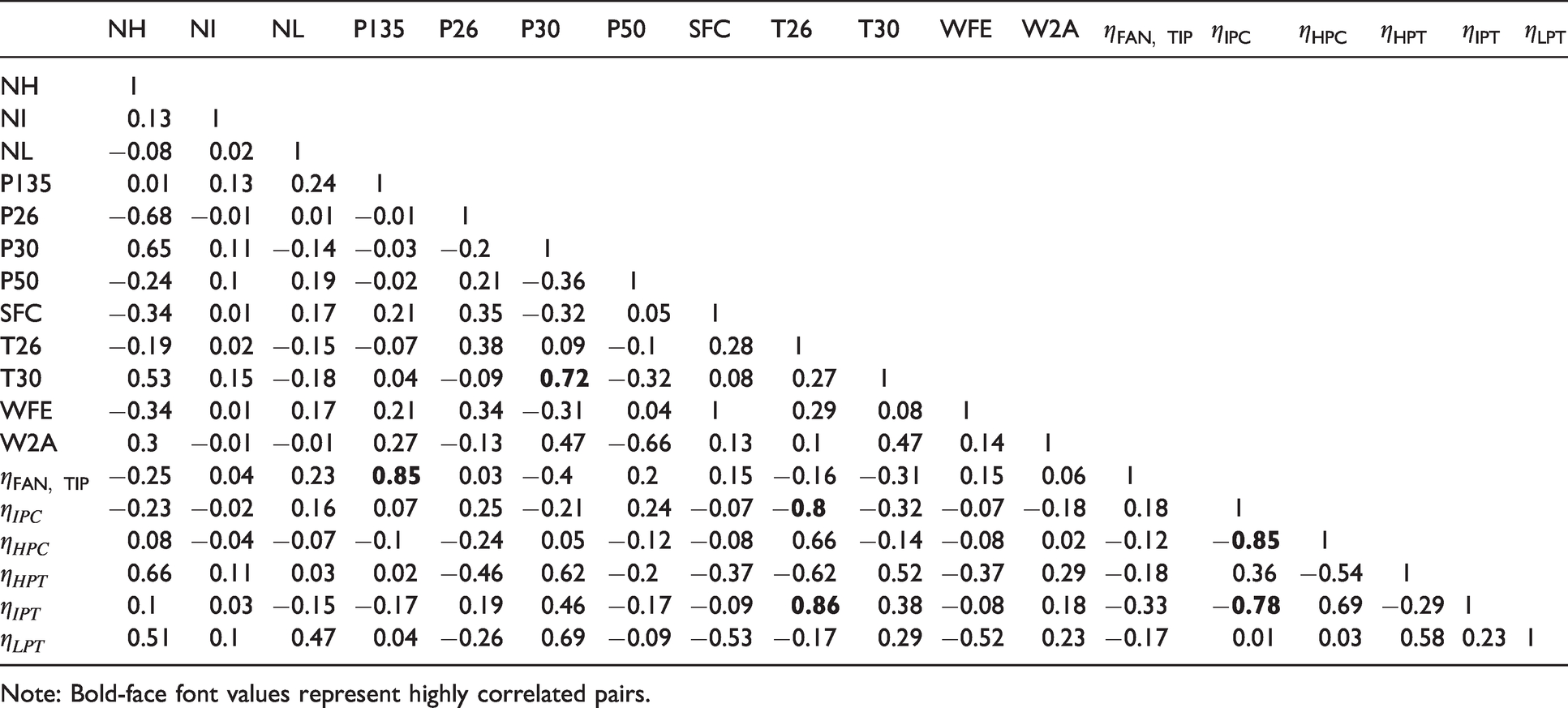
Note: Bold-face font values represent highly correlated pairs.

From Table 4, the high correlation of the fan tip exit total pressure P135 with the fan tip efficiency is expected. On the contrary, a correlation that should be considered is the P30 with LPT efficiency. This is not obvious and it should be further examined. Moreover, the T26 measurement is crucial as it is involved in the calculation of the core efficiencies. The correlations calculated indicate that as T26 increases, the Intermediate-Pressure Turbine (IPT) efficiency increases (corr = 0.86) and Intermediate-Pressure Compressor (IPC) efficiency decreases (corr=−0.8). This ‘reciprocal’ change in the gas path component efficiencies needs to be further examined.

Next, in order to accept an engine during pass-off testing, the performance parameters are monitored by analyzing their behaviour and trends. Different visualization techniques are being used, amongst them trend plots^27,28 and Cumulative Sum (CUSUM) plots.^29,30

Trend plots represent the mean engine performance and general scatter for each engine over a time period. They can be used in order to detect changes in components or measurement errors. The resulting performance trends allow the identification of changes in component performance or measurement instrumentation. The figures presented here represent the most useful trends. The measurements are first corrected to standard ambient and operating conditions¹ and the deviations are calculated relative to the nominal engine. Given a set of measurements, the engine performance model in ‘Analysis Mode’ is used to calculate the efficiencies of the gas path components.

A first important observation that can provide useful information is the detection of measurements that are constantly shifted. In Figure 5, it is observed that the HPC Inlet Total Temperature (T26) is constantly shifted by 1-1.5% from the reference engine. This is an important indication as a shift in measurement trends can be associated with an error in this measurement or fault in the corresponding components (IP spool). Specifically, this can be related to inadequate calibration of this sensor, leading to repeated readings of temperatures above the real one. Correspondingly, this can be also related to a change in the IPC efficiency resulting in higher exit temperatures and pressures. The same trend is observed for the HPC Outlet Total Pressure (P30) with a step-change in the deviation of this measurement around engine 200 (Figure 6).

Figure 5.

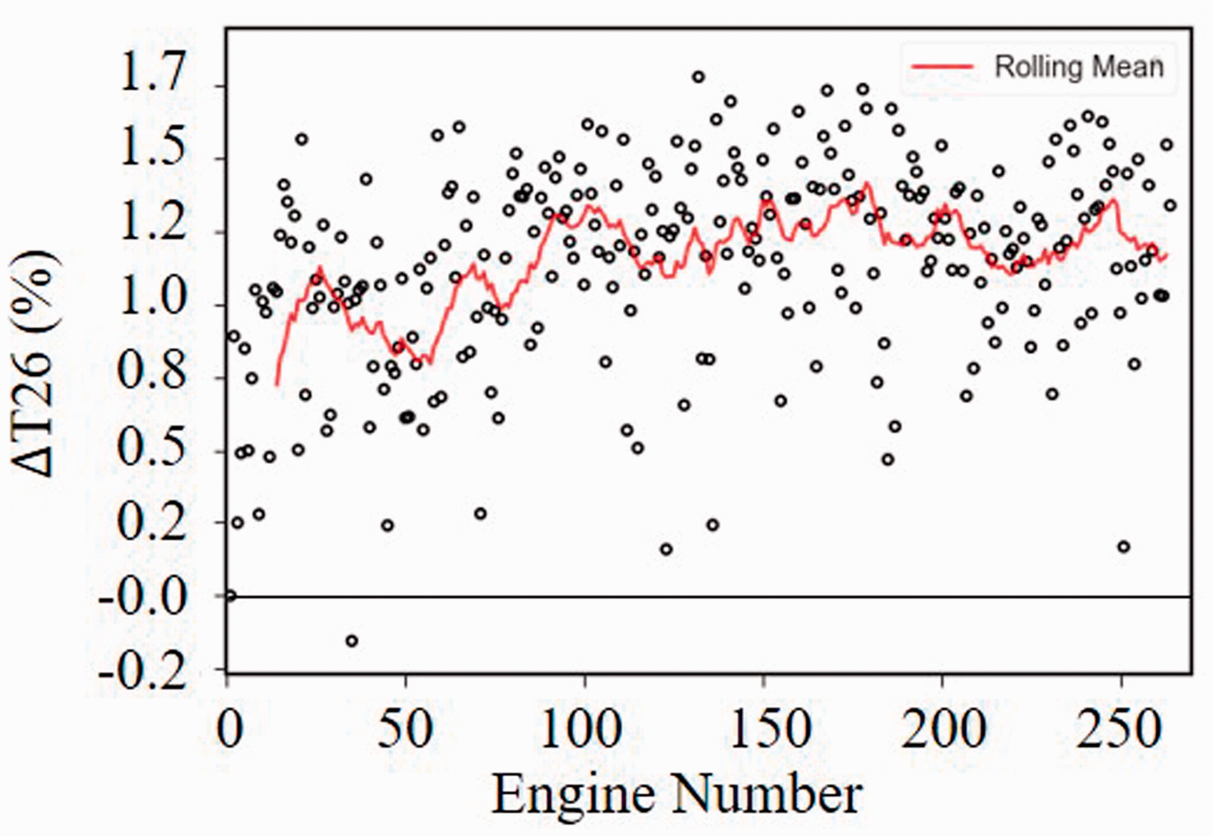
ΔT26 over engine number.

Figure 6.

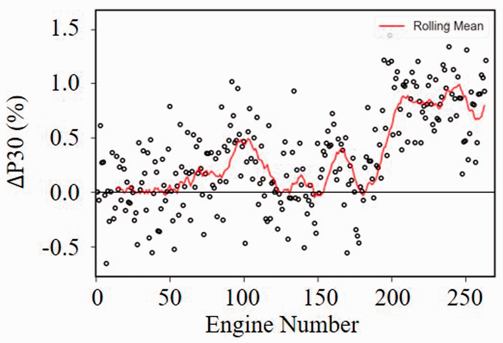
ΔP30 over engine number.

Another important observation that can be extracted from trend plots is the existence of potential step-changes. A step-change indicates that after a specific number of tests, there was a change/error in that specific recording. This can be often related to a change in slave set or to an unexpected error in measurement equipment. This concept can be clearly seen in Figure 7 where the deviation of LPT Exit Total Pressure (P50) ranges from -0.7% to 0.5% for the first 220 engines. An unexpected change is observed in the 221st engine, as the deviation increases instantly to approximately −1.5%. Similarly, a clear step-change is seen in the trend of the airflow (W2A) for the same observation (221st) (Figure 8). Specifically, before the step-change, the airflow was very close to the reference engine (−0.3%, 0.3%), while after the step the absolute deviation increases instantly to ≈ −1%. These two changes happening simultaneously can be explained by a change in the slave set. Testbed slave equipment includes both an intake and a nozzle. As a result, a change in slave set or its insufficient calibration will affect both measurements.

Figure 7.

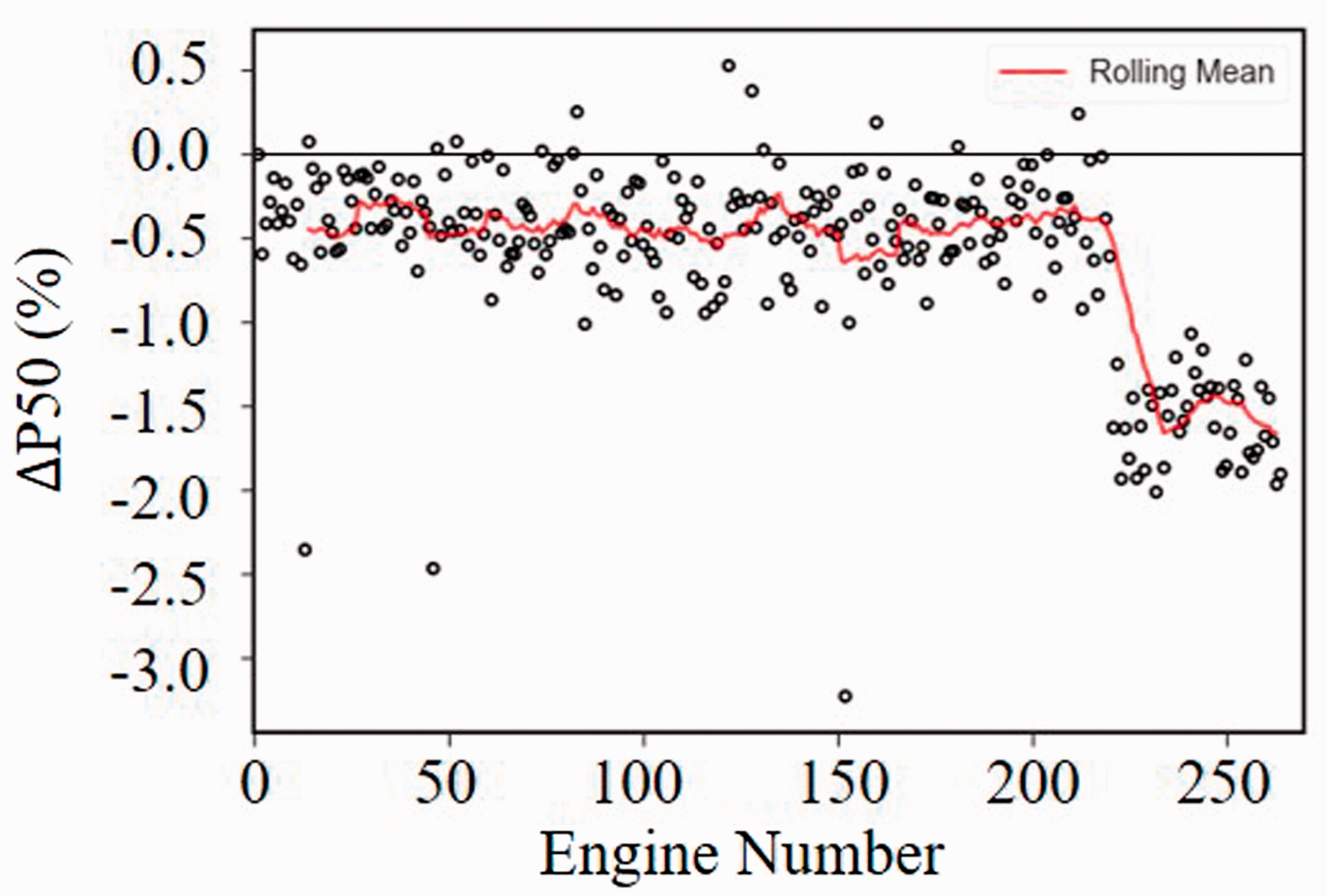
ΔP50 over engine number.

Figure 8.

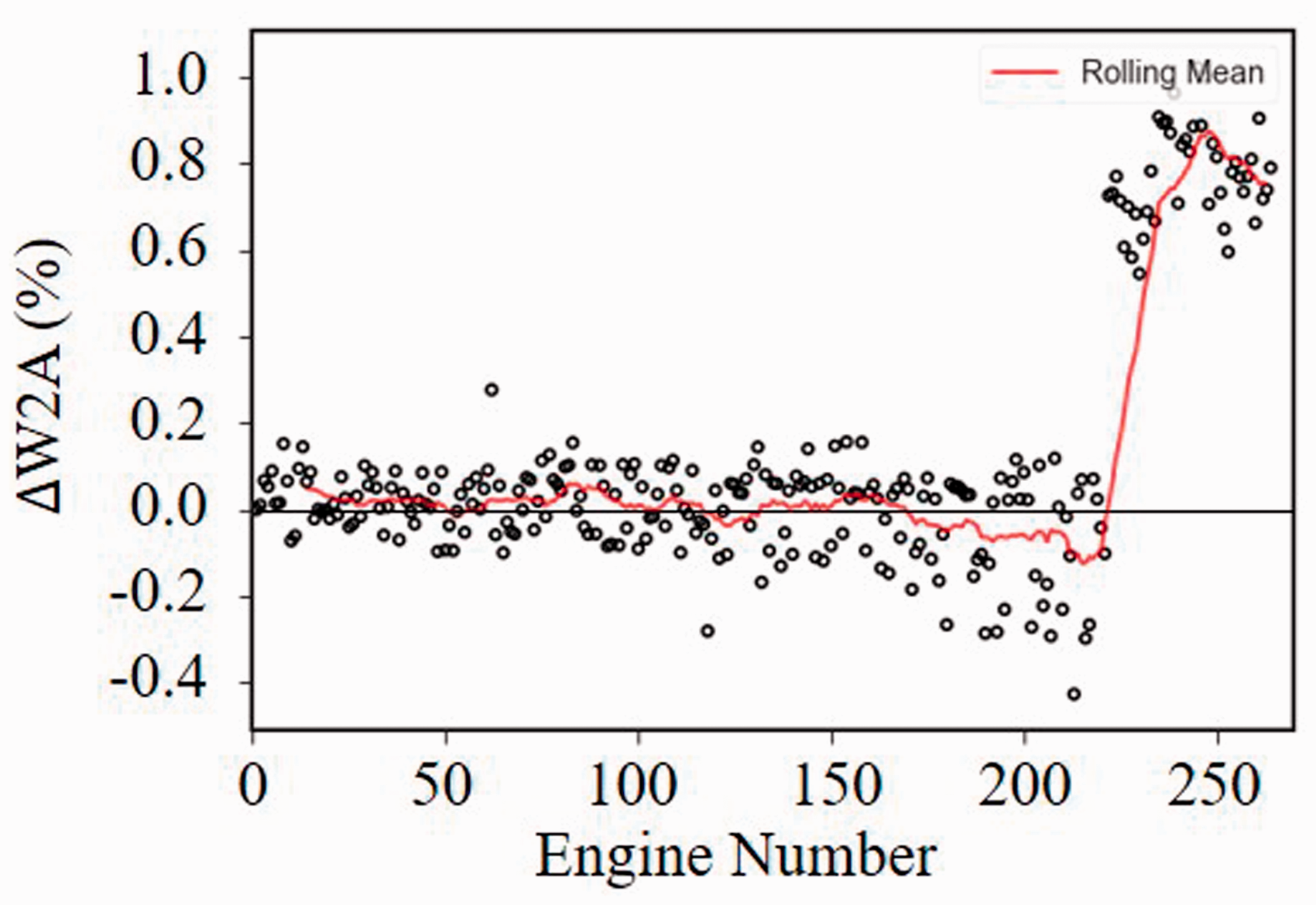
ΔW2A over engine number.

The apparent ‘reciprocal’ component changes are usually associated with single measurement errors.¹ The discussed concept can be observed in Figures 9 and 10, where IPC efficiency is repeatedly lower than the zero-deviation line (≈−1.8%) and IPT efficiency is repeatedly calculated high (≈+2%). This can also be seen in the correlation analysis, as the IPC and IPT efficiencies are highly correlated. The observed ‘reciprocal’ changes in conjunction with the shifted T26 measurement indicate that there is a measurement error.

Figure 9.

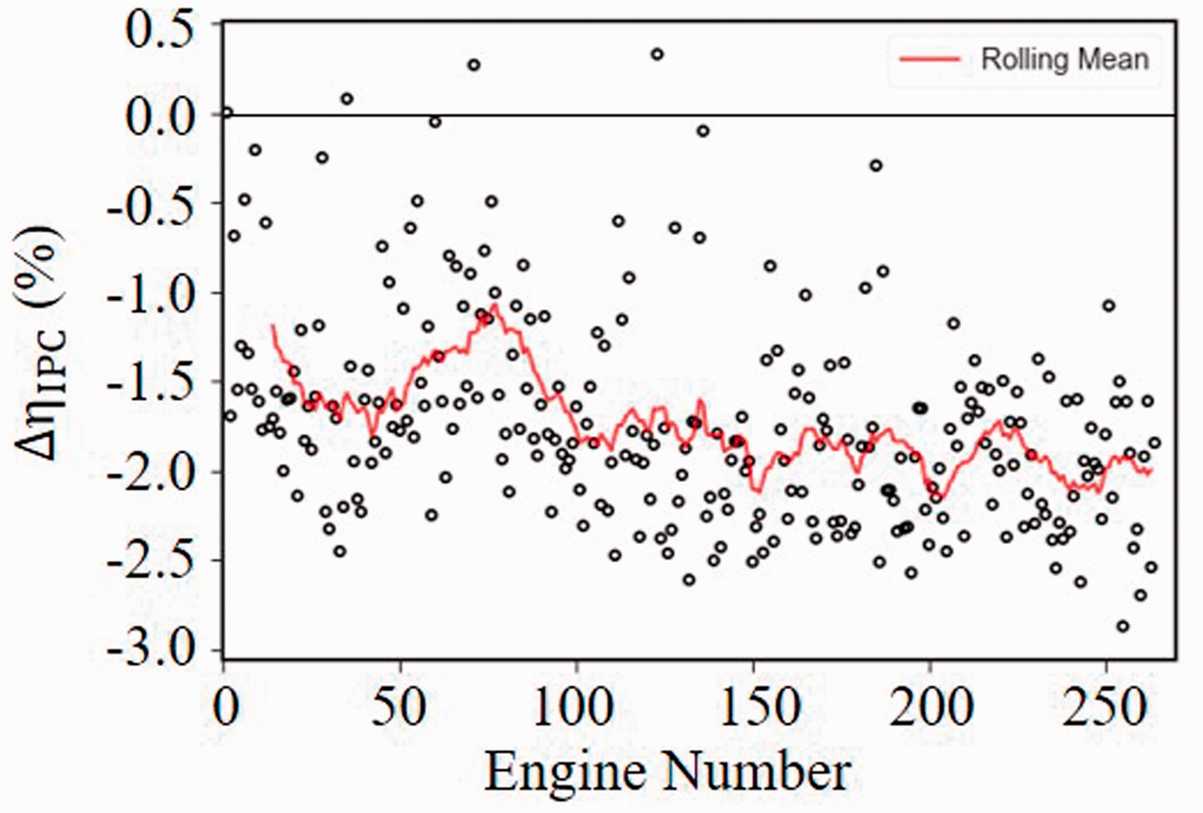
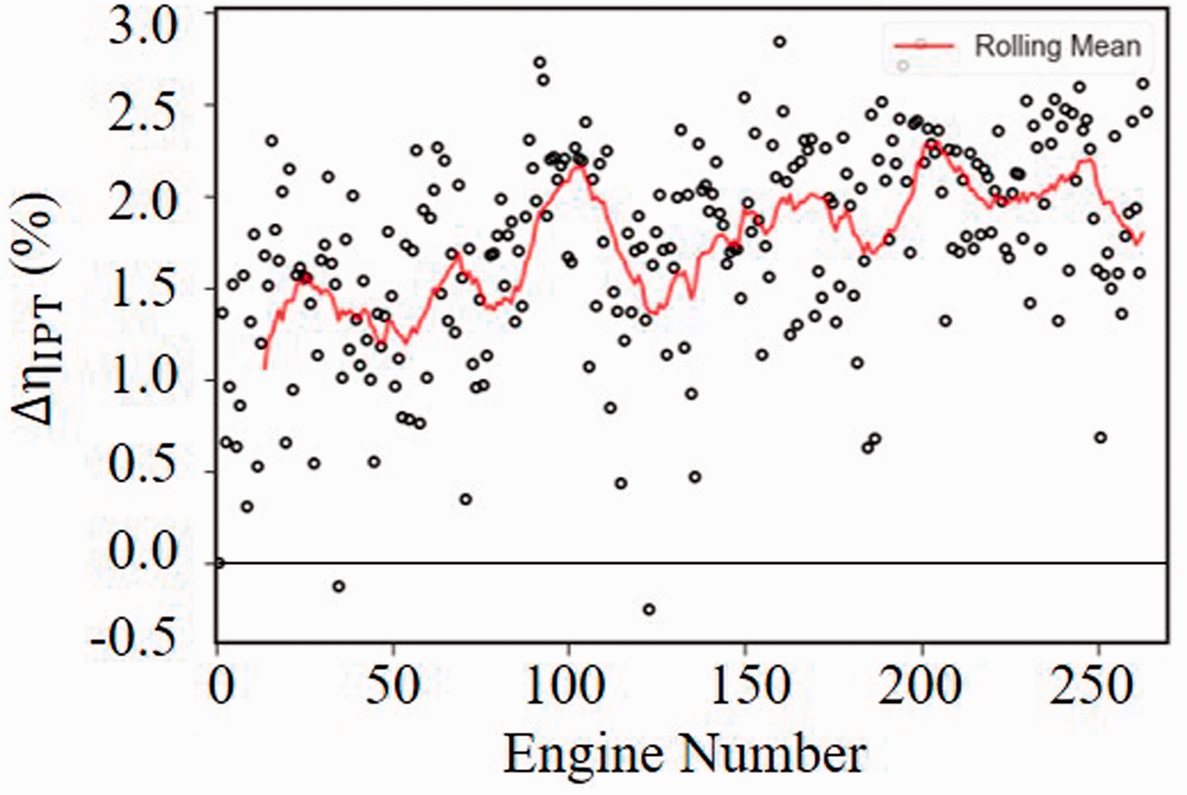
$Δ η_{IPC}$ over engine number.

Figure 10.

Δ $η_{IPT}$ over engine number.

Diagnostics results

The presented diagnostic method is applied to investigate the condition of 264 engines undergoing a pass-off test. Each production engine is tested once and hence optimization is carried out individually for each of the engines. Major assumptions in the current approach are that the engine model created is representative and that all the engines are identical in principle and hence, that the System Matrix C is derived correctly for all of them. The initial point for the optimization algorithm is selected to be a zero-vector representing the ‘datum’ component and sensor condition. For matters of interpretation, the results from the diagnostic tool are illustrated using scatter plots instead of the typical output file (Table 2).

The results of the analysis corresponding to the estimated measurement deviation are plotted for each engine recorded during the pass-off test. Estimated deltas equal to zero represent measurements and component parameters that remain unchanged.

Figure 11 outlines the predictions for the T26 measurement. The estimated bias for this measurement lies within the range of [0.6%, 1.8%] for all the engines. This indicates that the sensor is constantly reading higher than the reference value of T26. The measurement bias extracted from the diagnostic tool is ≈ 1.5%. Thus, the reference value of T26 is shifted. This error will later propagate in the calculation of the component efficiencies related to T26. Specifically, the IPC efficiency will be falsely calculated lower than the reference value, based on the calculations done using simulations in Analysis Mode. Similarly, the HPC efficiency will be calculated high while HPT will be calculated low and IPT will be calculated high. These trends in the core component efficiencies were also shown in the trend plots (Figures 9 and 10) and correlation analysis (Table 4). The main conclusion regarding the estimated error in T26 measurement is that in reality, the ‘reciprocal’ changes discussed earlier – four efficiencies shifted simultaneously – is an outcome of the propagation of the erroneous measurement in the calculation of those.

Figure 11.

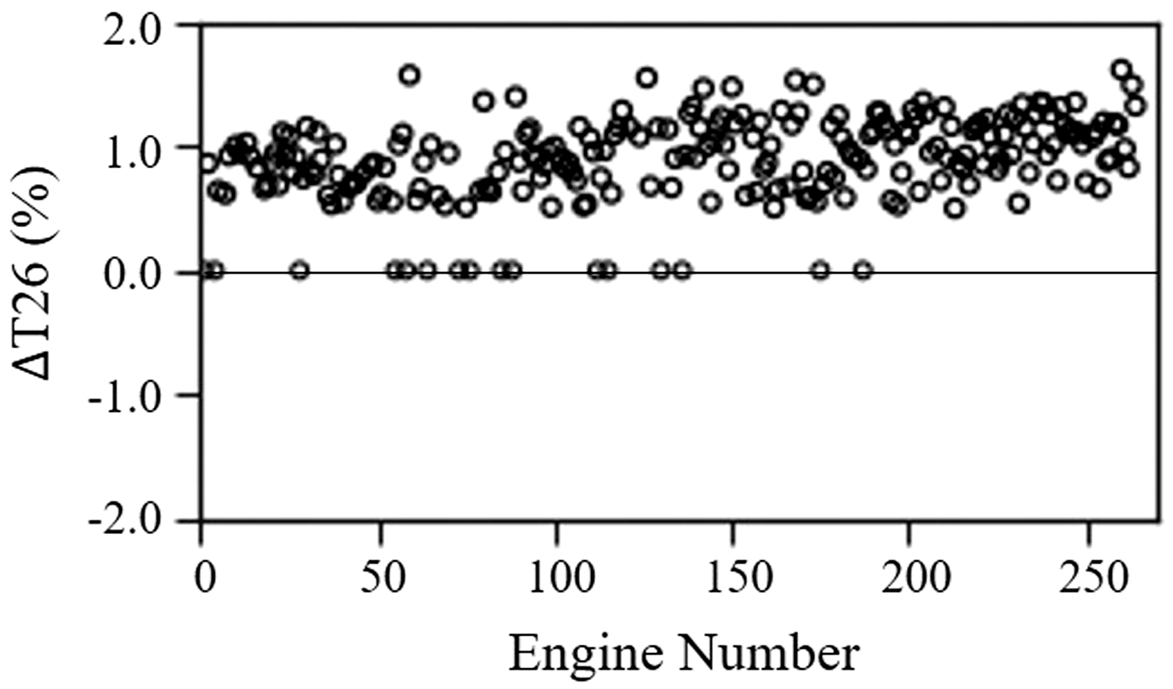
Diagnostic method results – estimated measurement error for T26.

Figure 12 illustrates the estimated measurement deviation for W2A. It is observed that the airflow appears to be consistently reading high after the 221st engine. The 221st engine corresponds to the beginning of the ‘step-change’ observed in Figures 7 and 8. This means that the actual airflow is lower than the measured one. Based on simulations running in the analysis mode, the calculated parameters, which are highly affected by airflow measurement, are the velocity and discharge coefficient of the by-pass nozzle. A W2A sensor that is reading falsely high will result in an increased velocity coefficient and a decreased discharge coefficient.

Figure 12.

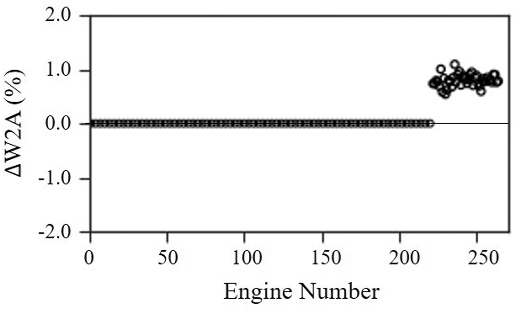
Diagnostic method results – estimated measurement error for W2A.

Although P50 is not measured during pass-off testing, analysis for P50 is included for completeness. P50 frequently appears to be read low (≈ −0.6%) before the step-change (Figure 13). It is noted however that after the step-change (221st observation), all the engines are affected by a P50 measurement shift of ≈ −1.6%. This means that the sensor is constantly reading lower than the real measurement after the step-change, and hence all the calculated parameters that are expressed as a function of P50 will be calculated wrong. A sudden shift in P50 bias may be a consequence of a change in the slave set (hot nozzle) or a change in calibration. As a result, the main conclusion regarding the P50 measurement is that after the 221st observation, the measurement is shifted.

Figure 13.

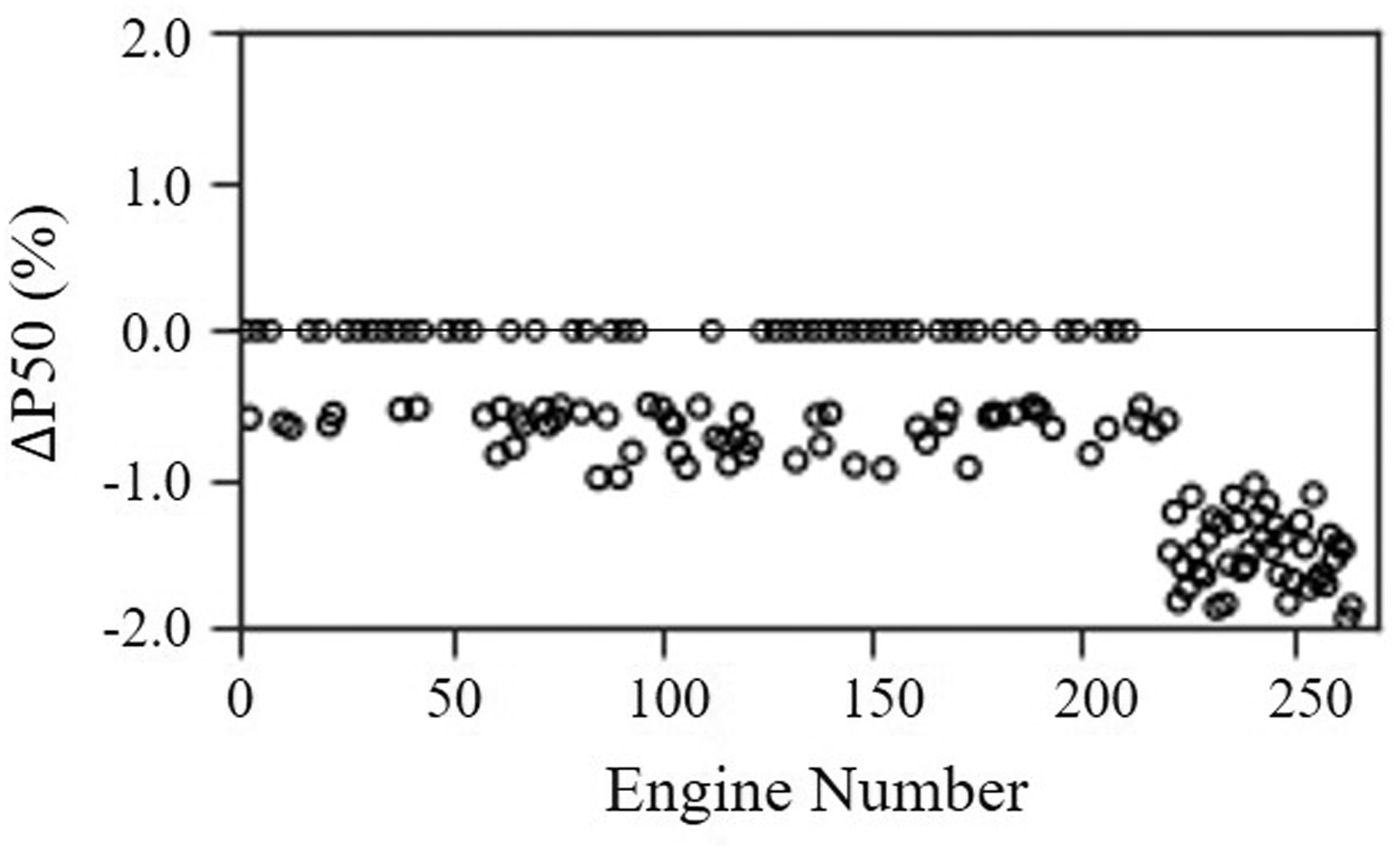
Diagnostic method results – estimated measurement error for P50.

It is noted that the simultaneous shift of both P50 and W2A is worth further examination as it can be an outcome of two possible conditions. Firstly, it can be a result of a change in the slave set. As previously stated, a slave set consists of a nozzle and an intake and hence, a change of slave set if not properly calibrated, can produce errors in both measurements. Secondly, in modern turbofan engines, P50 is often calculated based on the Analysis Mode instead of measuring it directly during pass-off testing. Assuming that this is the case, if W2A is erroneously read high, then the PR and the fan efficiency will also be calculated high. The fan will appear to absorb more power than the real. Therefore, the LP turbine will appear to have a higher specific work than the actual. This will result in calculating a P50 that is lower than the real one, which is the trend that we observe in the analysis. The reciprocal change of P50 and W2A strengthen the argument that P50 is calculated.

Additionally, Figures 14 and 15 show the estimated deltas for P30 and HPT capacity. After the 160^th observation, some production engines appear to have a P30 measurement error (≈ +1.2%) or P30 and some engines appear to be degraded, as HPT capacity is estimated low (≈ -1%). This trend indicates that the HPT capacity progressively reduces, and it might be worth investigating this change further.

Figure 14.

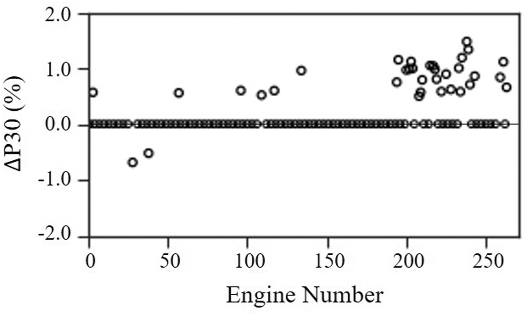
Diagnostic method results – estimated measurement error for P30.

Figure 15.

Diagnostic method results – estimated performance deterioration for HPT capacity.

Conclusions

In this paper, real pass-off test data from 264 three-spool turbofan engines were analyzed. Initially, a trend and correlation analysis was performed using the real data was performed. Next, a diagnostic method using a single objective optimization approach was implemented using a least-square-error (L2-norm) and a least-absolute-error type (L1-norm). The L1-norm was proven to be superior. It was shown that the utilization of this technique resulted in undesirable ‘smearing’ effects. For this reason, an enhanced method based on an alternative approach to the well-known Concentrator was proposed. This modification enables the potential to focus the optimizer onto a limited number of potential component changes and hence, eliminate the aforementioned effects. The method was shown to perform well and successfully predicted 82% out of the 405 simulated fault scenarios. The main advantages of the method are associated with the capability to account for both component degradation and sensor biases using only a limited number of measurements, without the necessity of a priori knowledge.

The proposed method was then applied to the production pass-off test data obtained for around 300 ‘identical’ engines. Although the observed variabilities were not critical to the pass-off process, understanding the behaviour of the population and the engine-to-engine scatter is considered of utmost importance. The variability observed during pass-off testing can be a consequence of many effects, such as genuine changes in engine components, measurement uncertainty, variability in day conditions which are not fully corrected out, changes in engine testbeds. The main conclusion from the analysis is that the engines that were showing variabilities during the pass-off process, were not subject to any component degradation. Instead, measurements that were used for the calculation of the overall engine performance were found to be erratic.

Although the present method was demonstrated on data from three-spool turbofan engines and a specific measurement subset, it can be used for different configurations and applications. It can be used for testbed data and pass-off test data analysis for new production engines or engines that have been overhauled. Additionally, it can be used for monitoring the deterioration of the performance of an engine during on-wing operation or testbed data and support maintenance planning.

Footnotes

Acknowledgements

The authors would like to express their gratitude to Rolls-Royce plc. for permission to publish the paper.

Declaration of Conflicting Interests

The author(s) declared no potential conflicts of interest with respect to the research, authorship, and/or publication of this article.

Funding

The author(s) received no financial support for the research, authorship, and/or publication of this article.

ORCID iD

Chana Anna Saias

References

Walsh

Fletcher

Gas turbine performance. 2nd ed. Great Britain: Blackwell Science Ltd, 2004.

Zedda

Singh

Gas turbine engine and sensor fault diagnosis using optimization techniques. J Propul Power 2002; 18: 1019–1025.

Marx

Kotulla

Kando

, et al. Comparison and synthesis of performance and aerodynamic modeling of a pass-off turbofan engine test cell. In: Proceedings of the ASME turbo expo 2015: turbine technical conference and exposition. Volume 1: Aircraft engine; fans and blowers; marine, Montreal, Quebec, Canada, 15–19 June 2015. New York: ASME.

Marinai

Gas path diagnostics and prognostics for aero-engines using fuzzy logic and time series analysis. PhD Thesis, Cranfield University, UK, 2004.

Kurzke

Halliwell

Model based performance analysis. In: Propulsion and power. Cham: Springer, 2018.

Provost

MJ.

The use of optimal estimation techniques in the analysis of gas turbines. PhD Thesis, Cranfield University, UK, 1994.

Kurz

Brun

Degradation in gas turbine systems. ASME J Eng Gas Turbines Power 2001; 123: 70–77.

Zaita

Buley

Karlsons

Performance deterioration modeling in aircraft gas turbine engines. ASME J Eng Gas Turbines Power 1998; 120: 344–439.

Dewallef

Romessis

Léonard

, et al. Combining classification techniques with Kalman filters for aircraft engine diagnostics. ASME J Eng Gas Turbines Power 2006; 128: 281–287.

10.

Urban

LA.

Gas path analysis applied to turbine engine condition monitoring. J Aircraft 1973; 10: 400–406.

11.

Mathioudakis

Kamboukos

Comparison of linear and nonlinear gas turbine performance diagnostics. ASME J Eng Gas Turbines Power 2005; 127: 49–56.

12.

Provost

MJ.

COMPASS: a generalized ground based monitoring system. In: AGARD conference preprint, Nr 448, 1988.

13.

Doel

DL.

TEMPER—a gas-path analysis tool for commercial jet engines. ASME J Eng Gas Turbines Power 1994; 116: 82–89.

14.

Volponi

AJ.

Gas turbine engine health management: past, present, and future trends. ASME J Eng Gas Turbines Power 2014; 136: 051201.

15.

Escher

PC.

Pythia: a n object-oriented gas path analysis computer program for general applications. PhD Thesis, Cranfield University, UK, 1995.

16.

Kalman

RE.

A new approach to linear filtering and prediction problems. ASME J Basic Eng 1960; 82: 35–45.

17.

Ganguli

Gas turbine diagnostics: signal processing and fault isolation. 1st ed. Boca Raton, FL: CRC Press, 2012.

18.

Provost

Nevell

DA.

Data processing system using a Kalman filter. US Patent 5105372A, 1992.

19.

Mathioudakis

Kamboukos

Assessment of the effectiveness of gas path diagnostics schemes. ASME J Eng Gas Turbines Power 2006; 128: 57–63.

20.

YG.

Performance-analysis-based gas turbine diagnostics: a review. Proc IMechE, Part A: J Power and Energy 2002; 216: 363–377.

21.

MacMillan

WL.

Development of a modular type computer program for the calculation of gas turbine. PhD Thesis, Cranfield University, UK, 1974.

22.

Stamatis

Mathioudakis

Papailiou

Optimal measurements and health indices selection for gas turbine performance status and fault diagnosis. ASME J Eng Gas Turbines Power 1992; 114: 209–216.

23.

Jasmani

Y-G

Ariffin

Measurement selections for multicomponent gas path diagnostics using analytical approach and measurement subset concept. ASME J Eng Gas Turbines Power 2011; 133: 05.

24.

Mathioudakis

Kamboukos

Stamatis

Turbofan performance deterioration tracking using non-linear models and optimization techniques. ASME J Turbomach 2002; 124: 580–573.

25.

Byrd

Hribar

Nocedal

An interior point algorithm for large-scale nonlinear programming. SIAM J Optim 1999; 9: 877–900.

26.

Stephen

BA.

Method. Patent EP2239642A2, UK, 2013.

27.

Aretakis

Roumeliotis

Alexiou

, et al. Turbofan engine health assessment from flight data. ASME J Eng Gas Turbines Power 2015; 137: 10.

28.

Koskoletos

Aretakis

Alexiou

, et al. Evaluation of aircraft engine gas path diagnostic methods through ProDiMES. ASME J Eng Gas Turbines Power 2018; 140: 121016.

29.

Larsson

Åslund

Frisk

, et al. Fault tolerant supervision of an industrial gas turbine. In: Proceedings of the ASME turbo expo 2013: turbine technical conference and exposition. Volume 4: Ceramics; concentrating solar power plants; controls, diagnostics and instrumentation; education; electric power; fans and blowers, San Antonio, TX, USA, 3–7 June 2013. New York: ASME.

30.

MF, Palme T, MG. A novel approach for gas turbine condition monitoring combining CUSUM technique and artificial neural network. In: Proceedings of the ASME turbo expo 2009: power for land, sea, and air, Orlando, FL, USA, 8–12 June 2009, pp. 567–574. New York: ASME.

Three-spool turbofan pass-off test data analysis using an optimization-based diagnostic technique

Abstract

Keywords

Introduction

Background

Gas turbine performance modeling and analysis

Review of GPA techniques

Scope of present work

Methodology

Engine performance simulation

Measurements and health indices selection

Diagnostic method

Formulation of diagnostic method

Selection of objective function

‘Concentrator’

Validation

Simulated case: Single component changes and sensor biases – Comparison of L1 and L2

Simulated case: Pairs of component changes and/or sensor biases

Application of the method to real engine pass-off test data

Pass-off real test data analysis

Diagnostics results

Conclusions

Footnotes

Acknowledgements

Declaration of Conflicting Interests

Funding

ORCID iD

References