Influence of fluid-structure interaction modelling on the stress and fatigue life evaluation of a gas turbine blade

Abstract

A computational method of fluid-structure coupling is implemented to predict the fatigue response of a high-pressure turbine blade. Two coupling levels, herein referred to as a “fully coupled” and “decoupled” methods are implemented to investigate the influence of multi-physics interaction on the 3 D stress state and fatigue response of a turbine blade. In the fully-coupled approach, the solutions of the fluid-flow and the solid-domain finite element problem are obtained concurrently, while in the decoupled approach, the independently computed aerodynamic forces are unilaterally transferred as boundary conditions in the subsequent finite element solution. In both cases, a three-dimensional unsteady stator-rotor aerodynamic configuration is modelled to depict a forced-vibration loading of high-cycle failure mode. Also analyzed is the low-cycle phenomenon which arises due to the mean stresses of the rotational load of the rotating turbine wheel. The coupling between the fluid and solid domains (fully-coupled approach) provides a form of damping which reduces the amplitude of fluctuation of the stress history, as opposed to the decoupled case with a resultant higher amplitude stress fluctuation. While the stress amplitude is higher in the decoupled case, the fatigue life-limiting condition is found to be significantly influenced by the higher mean stresses in the fully-coupled method. The differences between the two approaches are further explained considering three key fatigue parameters; mean stress, multiaxiality stress state and the stress ratio factors. The study shows that the influence of the coupling between the fluid and structures domain is an important factor in estimating the fatigue stress history.

Background

Gas turbine blades operate in a severe condition of high-pressure and temperature and as such, resonant vibrations are likely to occur with the newer designs incorporating the use of thinner airfoil profiles rotating at near sonic tip speed. ¹ The ensemble influence of the unsteady aerodynamics can induce some high-frequency, low-amplitude induced stresses. At resonance conditions, the stress magnitude increases proportionately with significant inelastic strains induced. The demand for improved component efficiencies therefore means that the components are designed optimally for reduced weight and higher blade loading leading to a closer axial spacing of the airfoils. These extreme design conditions therefore imply that the components are operating near their aeromechanical limits with increased risk of fatigue failure. The fatigue failures are mainly in the form of low-cycle and high-cycle fatigue conditions, and possibly creep with extended operation in high temperature and stress environment. In addition to fatigue failure, any form of external damage can also induce stress concentration at notch-like sites, and with the high rotation and temperature experienced at operating loads, is able to cause rapid failure of the blades. Nicholas ² presented a review on the high-cycle fatigue modes of gas turbine engine blades. Thus, the relevant structural issues present a unique problem case as the load pattern and the stress distributions are due to a complex interplay of aerodynamic, thermal and static structural loads. By its very nature, such problems lie in the domain of a coupled field analytical approach.

Of interest in this study is the influence of a coupled field simulation methodology on the stress and fatigue life evaluation of a gas turbine blade. Given that fatigue is the dominant failure mode observed for these components, its consideration in this study is limited to the dominant modes of high-cycle and low-cycle fatigue phenomena. In relation to the high-cycle failure mode, the unsteady aerodynamic of the stator-rotor configuration is able to excite the blade in one of its vibration modes, Fleeter et al. ³ A typical flow field is characterized by three-dimensional secondary flow features leading to spanwise pressure gradient in the blade. For a turbine stage profile running in a choked flow condition, the unsteady Mach wave can lead to a high amplitude pressure fluctuation within intra blade row passages and on the downstream components. Correspondingly, for the low-cycle fatigue condition, the material response is characterized by repeated cyclic hardening and softening, as evident on the cyclic hysteresis loop. Previously, research efforts have been focused on understanding this complex failure modes. Hou et al. ⁴ presented a combined low-cycle and high-cycle fatigue for nickel-based turbine blade single crystal material. The life estimation model was based on a power law crystallographic model, again, taking into consideration the resolved shear stress under first-order vibration loading. The high frequency low-amplitude stresses from the unsteady aerodynamics were not considered in their study. Bernstein and Allen ⁵ presented a fatigue analysis of a cracked turbine blade. The cracks were observed along the leading edge and mid-chord regions of the airfoil pressure and suction surfaces, and were attributed to the severe stresses induced during the start-up and shut-down cycle operation, which are typical low-cycle fatigue inducing phenomena. The cracks noticeable on the pressure side were explained in relation to the complex biaxial stress state estimated at the mid-chord section where the maximum principal stress state was shown as the dominant parameter influencing the crack propagation direction.

Prior to the implementation of the elaborate fatigue life tool, an accurate estimation of the response input stress history is important. It is necessary that after each start-stop cycle, the operator understands the need for scheduled servicing following a certain number of operating hours. The underlying assumption here, is that the numerical interaction between the thermal, aerodynamic and rotational loads, for which a typical turbine blades operate in, affect the stress response of the blades. The interplay of these loading conditions is difficult to replicate in a typical laboratory test environment. However, with increasing computing power, the associated loading conditions can be analyzed on a finite element basis, enabling designers to have a prior knowledge of possible notched-like locations of high-stress concentrations. In addition, the recent improvements in the development of these solvers, enable a close-to-ideal model to be replicated in a way to help the further understanding of the dominant damage modes at the design phase. This is important given that for a critical component such as the high-pressure turbine blade, an inaccurate life estimation can lead to an overly expensive designs, or that due to underutilization of remaining useful life, Halford et al. ⁶

In this study, a numerical approach of fluid-structure interaction is implemented to investigate the influence of multi-physics coupling on the load response and fatigue life of high-pressure turbine blade. Fluid-Structure Interaction (FSI) is a multidisciplinary solution approach which considers the interaction between the two fields of fluid and structural response. Such complex formulation of the interaction between the two-fields have been aided by the separate development of the finite element and computational fluid dynamics codes, previously allowing them to be treated separately without any form of multi-physics interaction. Although studies have been performed highlighting the application of fluid-structure interactions to turbine blade problems, ¹ very little information exist on the influence of this higher-fidelity and computationally expensive approach on the solution procedure, nonetheless, in relation to fatigue life estimation. Two numerical approaches are formulated herein, referred to as a “decoupled” and “fully-coupled” method, depending on the order of interaction between the fluid and solid domain fields. In the fully-coupled method, the solutions of the solid mechanics equations and the compressible fluid solution are obtained simultaneously. The decoupled (one-way) method is the classical analytical approach where the fluid pressure loads are computed initially, and subsequently transferred to a solid domain finite element approach for the estimation of stresses in a separate analysis. A significant parameter often not considered in this approach is the clear estimation of the effects of the unsteady flow fields on blade vibrational levels and vice versa. The method calculates the aerodynamic forcing and damping terms independently, and the resulting aerodynamic forces are subsequently applied as load boundary conditions in the follow-up structural analyses. The assumption of this approach is based on previous understanding that the mode shapes remain unchanged in the case of lightly damped turbomachinery blades.^7,8 This current work therefore shows that even for low-aspect ratio profiles, typical of a high-pressure turbine blade, the effect of multi-physics interaction is essential in the estimation of stress history prior to an elaborate fatigue life estimation.

Fluid-structure interaction (FSI) and modelling approach

The interplay of the loading conditions of an engine blade can be described using the numerical approach of fluid-structure interaction. Fluid-structure interaction describes a field of multi-physics coupling with mutual interaction between the fluid and the solid domain, Bazilevs et al. ⁹ A review of its application on the aeroelastic investigation for turbomachinery applications was given by Marshall and Imregun. ⁸ In a typical turbine stage, the interaction of these high-amplitude unsteady pressure signals with the displacement from the rotational load, is able to feedback some damping to the overall blade response which can only be predicted in a fully coupled, fluid-structure model framework. As reported by Srinivasan, ¹⁰ the loading condition of a turbine blade requires the simultaneous coupling of the flow governing equations to that of the finite element structural model. This is based on the understanding that the extent of the aerodynamic damping superimposed on that from the non-aerodynamic sources would result in the prediction of the true stress state of the blades. This approach is therefore formulated in this study, analyzing a full 3-D unsteady transient flow and solid domain under a fully-coupled simulation framework. This is illustrated in the flow chart of Figure 1.

Figure 1.

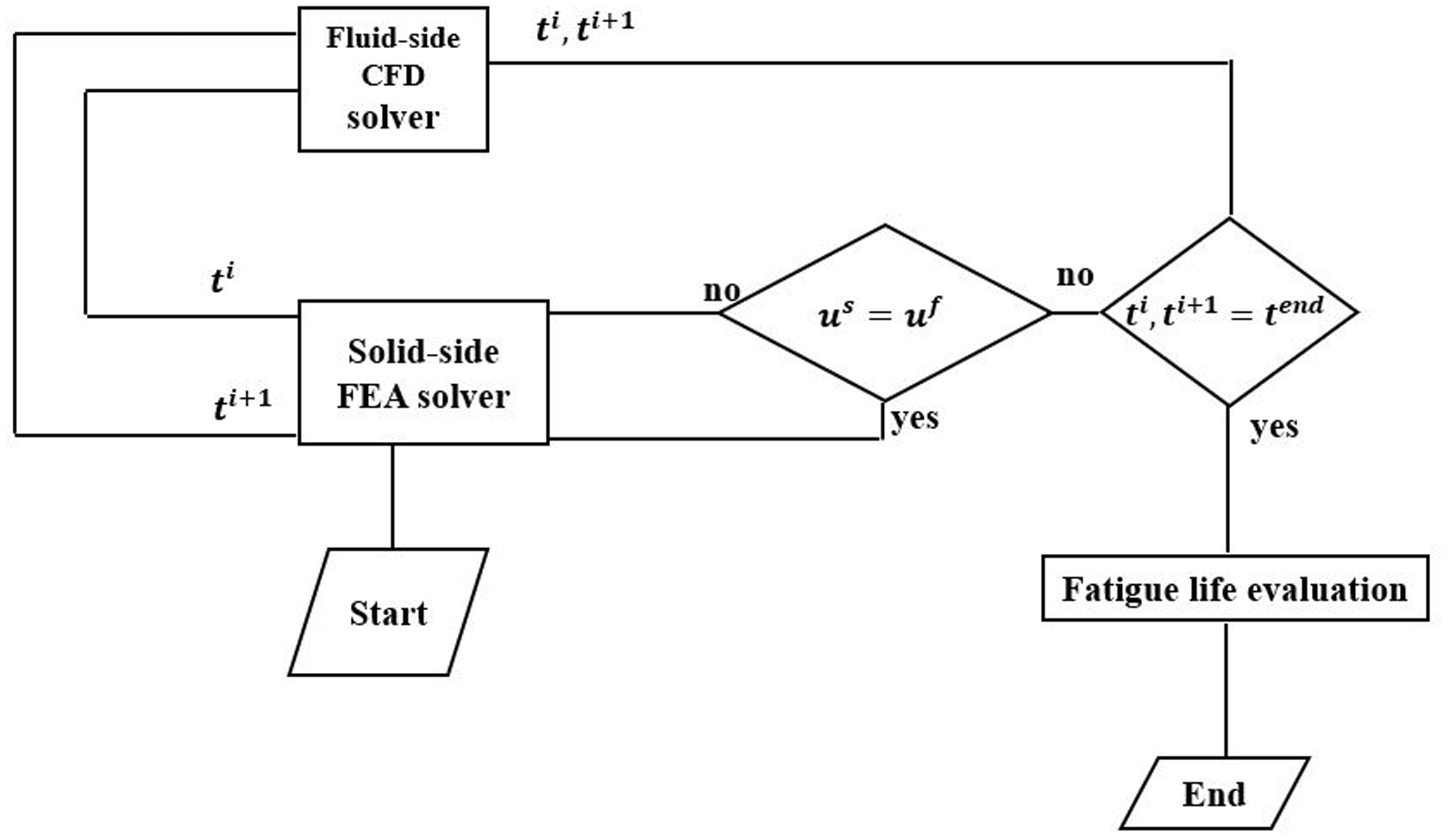
Fully coupled simulation approach.

In the fully-coupled method, the fatigue life input stress history is obtained through a simultaneous solution of the blade structural equation of motion and that of the fluid flow. The fluid and solid side meshes at the interface boundary are updated via feedback loops ( $t^i,t^{i+1})$ that couple the two solvers per solution timestep. A maximum of 10-coupling steps is implemented to ensure that the transfer of variables between the solvers satisfy the requirement of conservation and compatibility conditions at the interface. This is invariably a tight coupling procedure and the formulation allows for an automatic inclusion of the aerodynamic damping term, which is often separately estimated in the unilateral data transfer approach of the decoupled method. The only difficulty associated with the fully coupled method is the longer computation time that is required to obtain a fully converged solution, given that a minimum level of 3-iterations is necessary to ensure a tight convergence per solution timestep. There is also the need for constant updating of the fluid-and solid-side meshes at each solution step.

In the implemented fully coupled method of this work, the structural deformations induce a moving boundary in the fluid domain and vice versa. It is therefore necessary that the fluid mesh be formulated to match the current position of the solid interface at each solution step. Following the method stated in Dinkler et al., ¹¹ the use of an iso-parametric space-time element enables the specification of mesh displacement at arbitrary location, for which case, the fluid model can move with the structure. Therefore, the need for maintaining compatibility at the fluid-solid interface is ensured through an iterative multi-stepping of solution variables for each time step. Also, in order to avoid the distortion of the fluid-side elements, a specification of an element-wise constant stiffness distribution as a function of the smallest edge length of each element was implemented.

An additional requirement is the need to maintain the kinematic compatibility condition at the fluid-solid interface. At the fluid-solid interface, the kinematic condition assumes the continuity of the velocity field at the interface. For a viscous flow case, this is represented in the form:

$$T_r{\left(U^s\right)}_{|\mathrm{\Gamma }}=T_r{\left(U^f\right)}_{|\mathrm{\Gamma }}$$

(1)

And for an inviscid flow case;

$$T_r{\left(U^s.n\right)}_{|\mathrm{\Gamma }}=T_r{\left(U^f.n\right)}_{|\mathrm{\Gamma }}$$

(2)

where “ $T_r$ ” is the trace operation signifying the restriction applied to the interface, and “ $U^f$ ” is the surface variable at the fluid interface. “ $U^s$ ” is the corresponding variable on the solid-domain interface, and $n$ is the unit normal vector. Similarly, in maintaining the energy balance at the interface boundary, the related dynamic conditions are maintained through the relation:

$$d_f=d_s$$

(3)

$$n_f.{\tau }_f=-n_s.{\tau }_s$$

(4)

where $d_f,d_s$ are the respective fluid-side and solid-side displacement conditions. Also, ${\tau }_{f,}{\tau }_s$ are the shear stress tensors in the fluid and solid-side models, and $n_f,n_s$ are the unit normal vectors pointing outwards from the fluid and solid domains, respectively. The benefit of the implemented method is that the separate gauss integration points can be chosen independently for the fluid and solid stiffness matrices. The method ensures energy conservation in the fluid-solid interface, Γ, through its computation of surface traction (moments and forces) parameters.

In the second analysis method of decoupled (one-way) approach (Figure 2), the unsteady aerodynamic analysis is performed independently, and the estimated pressure fields are transferred as boundary conditions to the solid finite element model. The method is performed without any feedback loop between the two fields as the two solutions are obtained separately. The argument in support of this method is its simplicity in implementation as most commercially available solvers have this capability. The method is readily implemented with reduced computational time, given that no sub-cycling within each timestep is required to ensure conservation and compatibility condition, as is required of the two-way method. As such, the decoupled method allows the use of separate solvers without the need in formulating an interface/coupling algorithm to couple the independent codes. ⁶ The decoupled approach as implemented in the current analyses involves a single execution of the fluid and solid-side model equations.

Figure 2.

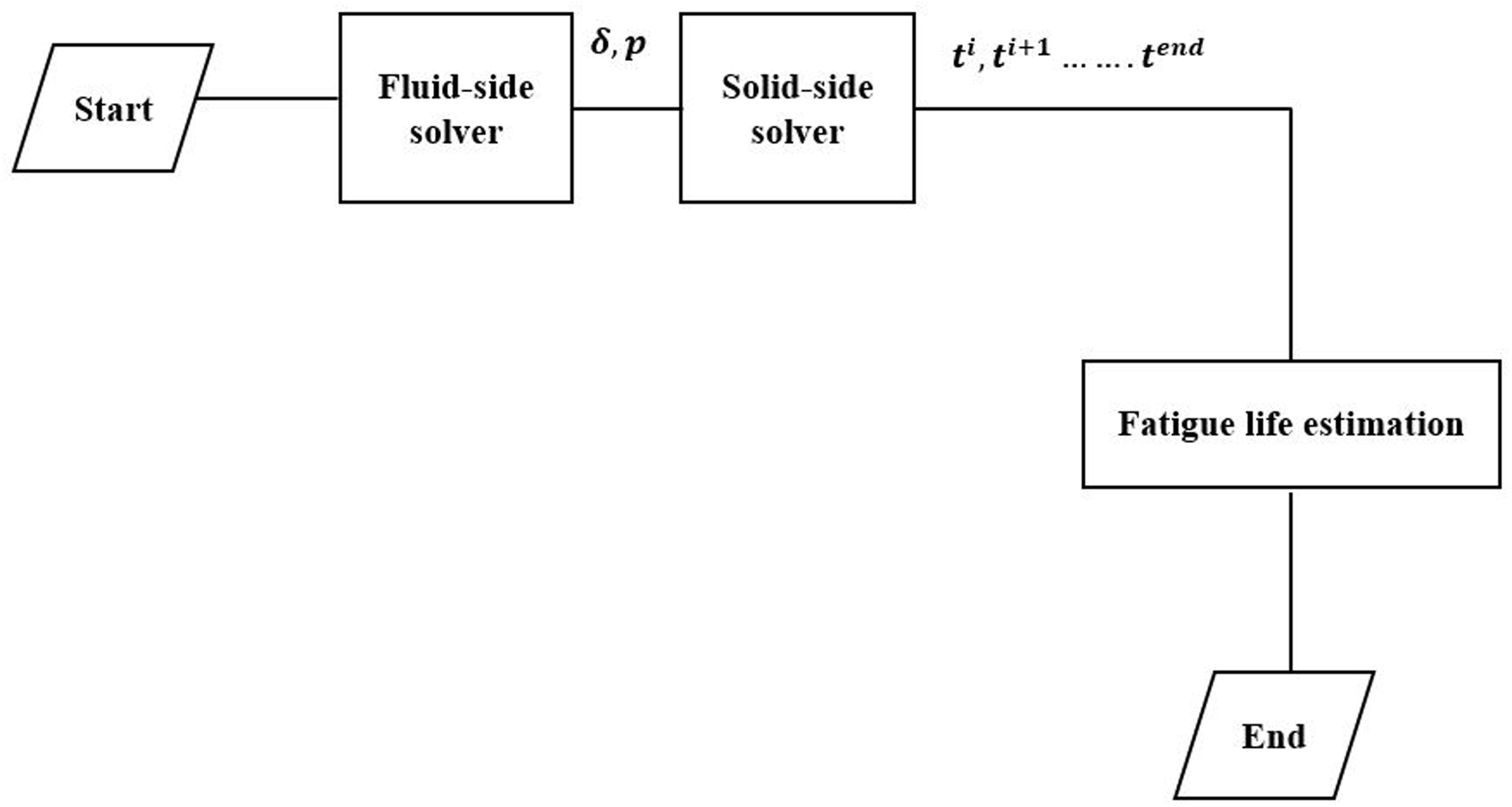
Decoupled solution method.

As shown in Figure 2, a key parameter in this approach is the accurate estimation of the aerodynamic damping term. The total damping sources on a turbine wheel is mainly of three types; mechanical, aerodynamic and material. The mechanical damping sources are the friction dampers, and this is not considered in the current study, as only the blade airfoil model is analyzed without the fir-tree attachment. The material sources are from the implemented temperature properties of stainless steel 304LC. Correspondingly, the aerodynamic damping source was estimated using the log-decrement method of the form;

$${\zeta }_{\mathit{aero}}=\frac{\delta }{\sqrt{4\pi +{\delta }^2}}$$

(5)

where $\delta$ is the log-decrement value obtained by averaging the peaks and successive peak values of the unsteady pressure signal. A similar method for estimating the damping of a turbomachinery blade undergoing multiple vibration modes was reported in Gottfried and Fleeter. ¹² Using the above correlations, the decoupled approach estimated an averaged aerodynamic damping coefficient of 0.006. from the unsteady pressure signals.

Solver implementation

Fluid flow formulation

The fluid-side computations of this work were implemented using the CFX package. Herein, the flow governing partial differential equations are solved using the finite volume approach to transform the relevant equations into balance equations over a structured mesh cell element. With the use of the Gauss divergence theorem, the volume integrals of the divergence of the diffusion and convection terms are transformed into surface integrals over the elements. The conservative property of the method is ensured through the computation of the surface fluxes at the element faces. An extensive discussion and derivation of this method was given in Hirsch ¹³ and Moukalled et al. ¹⁴ For a scalar flow variable $\mathrm{\varnothing }$ , the generic conservation equation can be represented in the form;

$$\frac{\partial \left(\rho \mathrm{\varnothing }\right)}{\partial t}+\nabla .\left(\rho V\mathrm{\varnothing }\right)=\nabla .\left({\mathrm{\Gamma }}^{\varphi }\nabla \mathrm{\varnothing }\right)+Q^{\varphi }$$

(6)

In its current form, the above equation requires the fluxes to be differentiable which makes it restrictive as compared to its integral representation. However, this derivative form allows it to be locally valid in any point in the flow domain. The terms on the left-hand side are the transient and convection terms, respectively. The respective terms on the right-hand side are the diffusion and source terms. A vertex-centered finite-volume is implemented which can handle any non-orthogonal regions of the mesh during the discretization of the diffusion term (viscous shear stresses). Although in a single-phase fluid problem of this formulation the diffusion term is not explicitly present, the presence of viscous shear stress from the turbulence closure models will clearly exhibit the characteristics of a diffusion flux. ¹³ As such, for the variation of flow variable, $\varphi$ over a cell face, the corresponding gradient term was solved using the least-squares approximation technique. At each solution iteration, the face average value of the scalar variable $\mathrm{ }\varphi$ was predicted from the gradient computation of the previous solution step. For the convection term, a high-resolution scheme was implemented using the Total Variational Framework (TVD) approach. This uses a combination of a high-order profile and a convection bounded criterion to prevent oscillatory behavior of the solution. Based on its formulation, the TVD framework preserves monotonicity by adding the product of an anti-diffusive flux and a flux limiter scheme to a diffusive first order upwind scheme. The procedure for its implementation in a finite volume solver was reported in Moukalled et al. ¹⁴ The specification of a wall condition on the blade surface sets the normal velocity at the wall to zero. This also reduces the convective flux to zero and as such, is eliminated from the algebraic equation. The transient term was matched in time using the second order upwind Euler scheme. The complete linearized systems of algebraic equations are solved using the iterative solver option with the algorithm repeatedly applied until a set limit of convergence is reached. The resulting linear equations from the discretization process was solved using the conjugate gradient method (a type of the iterative solution approach). The convergence criterion was set when changes between successive iterations reached 1e-04.

For the fully-coupled case, the stability of the coupled iteration was ensured by increasing the under-relaxation factor to 1, which conventionally implies a little under relaxation as was obtained from prior calculation on similar problem. Given the highly turbulent nature of turbine flows, the SST $k-\omega$ model was implemented. This was formulated to provide an improved pressure gradient performance, in comparison with the eddy-viscosity models. Similarly, the principal shear stress and the turbulent kinetic energy in the near wall, boundary layer region was modified by bounding the turbulent viscosity term from the proposed blending function of Menter. ¹⁵ A similar blending function to that of the eddy-viscosity model enables the $k-\omega$ to be able to model free-shear flows. In the current case of a compressible flow problem, the necessary boundary conditions to be imposed were set by the Mach number range of flow. Therefore, at the stator-inlet boundary, stagnation pressure and temperature values were imposed with the inlet treated as a Dirichlet boundary condition. The fluid transitions from static to stagnation state through an isentropic process, where the total-to-static pressure ratio is related to temperature ratio using the isentropic relation.

For the rotating rotor blade domain, the composition law sums the two velocity components, which are made of a relative component and the entrainment component. Given that the entrainment component has a negligible influence on the mass balance of the system, the corresponding continuity conservation equation remains unchanged in relation to the fixed (stationary) frame. However, for the momentum conservation equation, the inertia terms takes into account two forces on the right-hand side of the equation; the Coriolis force per unit mass $-2\left(\overrightarrow{\omega }\mathrm{ }\times \overrightarrow{V_r}\right)$ and the centrifugal force per unit mass $\left({\omega }^2\overrightarrow{R}\right)$ , where $\omega$ is the rotor angular speed, $V_r$ is the relative velocity in the rotor frame and $R$ is the position vector perpendicular to the axis of rotation. In a similar way, the energy conservation equation is modified to consider the work due to the centrifugal forces only. Coriolis forces have negligible impact on energy balance of the flow. The implemented solution considers the moving grid effect due to the solid-side displacement. The scalar conservative equation is modified to account for the relative flux vector which is obtained from the surface integral of the product of the scalar variable, unit normal vector and time-stepping parameter. The same approach is extended for a vector quantity, such as momentum, by introducing a relative convective flux tensor. ¹³

A domain interface condition was maintained at the periodic boundaries, as well as at the stator-rotor interface boundary. This was modelled to allow for changes in the frame of reference between the two domains. The interface condition was that of the Generic Grid Interface (GGI) mesh connection method, which allows for differing areas on both sides with mutually overlapping boundaries. Given that the stator-rotor interfaces do not exactly match due to the pitch angle differences, a multiple frame of reference (transient rotor-stator) boundary was implemented to account for the time-averaged interaction effects. This provides a circumferential averaging of the fluxes at the domain interface. In the current work, a single-passage analysis is performed in order to reduce the computational resources as required for a full wheel analysis. The formulation of a single passage analysis assumes that the test configuration exhibits cyclic symmetry with $N$ identical replicas that close to form a wheel with a phase-shifted periodic boundary condition. This enables a reference sector defined by a sector angle of $\beta =\frac{2\pi }{N}$ to be modelled. ¹⁶ As noted by Su et al., ¹⁷ this assumption allows for the simplification of the computation domain of the unsteady aerodynamic of the annular cascade to a single blade passage. These assumptions, however, are likely to be violated in models with significant amount of mistuning present between the component blades of the turbine wheel. ¹⁸

Solid-side finite element formulation

On the solid-side finite element model, the problem was formulated following a forced response procedure with the bounding equation of motion of the form:

$$\left[M\right]\left\{\ddot{x}\right\}+\left[C\right]\left\{\dot{x}\right\}+\left[k\right]\left\{x\right\}=\left[R\right]$$

(7)

This represents a system of differential equation of second-order with an applicable standard solution procedure of either the direct integration or the mode superposition techniques as described in Bathe. ¹⁹ In equation 7, the terms $\left[M\right],\mathrm{ }\left[k\right]$ are the mass and stiffness matrices, respectively, for a blade nodal number, $\mathrm{ }n,$ of a certain model eigenvector, $\left\{{\varphi }_i,n\right\}$ . The term $\left[R\right]=\left[F_A\right]+\left[F_R\right]$ represents the external forcing vector, and includes $F_R,\mathrm{ }$ the forcing vector to account for the coriolis effect due to the high rotational speed and $F_A$ , that of the unsteady aerodynamic forces. Due to the effect of rotation, the overall system stiffness matrix was represented in the form, $\left[K\right]=\left[k_{el}\right]+\left[k_r\right]+\left[k_l\right]+\left[k_g\right]$ . This accounts for the influence of the elastic, rotational, pre-strain and geometric stiffness terms, respectively. Also, the damping matrix $\left[C\right]=\left[c_{st}\right]+\left[c_r\right]+\left[c_{\mathit{aero}}\right]$ ; includes the effect of structural, damping and coriolis effect, and the aerodynamic damping effects. The structural damping terms are inherently estimated from the specified material conditions and rotational speed. The aerodynamic damping term was estimated from the monitored unsteady pressure signals on the rotor blade. The solid blade model in the finite element solver was discretized with the SOLDI227 tetrahedron element. This has ten nodes with five degrees of freedom per node. Being a multiphysics element, it also suitable for other coupled-field analyses such as the thermoplastic analysis with capability for creep strain and large deformation cases. ²⁰

The above equation of motion can be solved either through the direct integration (implicit or explicit solution approach) or the modal superposition methods. The required initial conditions are the displacement and velocity condition at time, t = 0, for a transient case. In the direct integration approach, the timestep specification has a significant role on in the selection of the numerical scheme. The choice of a reduced timestep would mean that higher frequency responses are not accurately resolved as these require longer period to fully integrate the stiffness in the equation of motion. On the other, higher timestep can lead to numerical instability of explicit solution schemes. As implemented in this study, the direct method offers no transformation of the equation of motion into a different form prior to the numerical integration process. The modal superposition method, however, is best suited for linear analysis while the direct integration methods (explicit and implicit schemes) are often used for nonlinear cases Noh and Bathe. ²¹ In the current analysis, an implicit backward Euler direct integration approach was adopted for the solution of the nonlinear finite element problem. By nature of its formulation, the implicit backward Euler scheme is capable of treating inertial problems and the modeling of such complex geometry as a turbine blade in three-dimension. ²² The method is unconditionally stable and involves the solution of structural stiffness for every timestep. The corresponding influence of the timestep selection is evident in the solution accuracy and does not affect the numerical stability of the solver, as opposed to its effect in explicit schemes. While this is true generally for implicit schemes, the current implementation with multi-physics interaction shows some instabilities in the predicted solution of the fully-coupled case, where a strong coupling is ensured between the fluid and solid-side equations. As noted by Liu et al., ²³ one of the attractive features of the backward Euler method is its wide applicability on linear and nonlinear analyses type problems.

Assuming the solution at prior timestep, $t=0$ is known, the model equation for the current timestep, $t+\Delta t$ , is formulated in the form;

$${\left[M\right]}^{t+\Delta t}\left\{\ddot{x}\right\}+{\left[C\right]}^{t+\Delta t}\left\{\dot{x}\right\}+{\left[K\right]}^{t+\Delta t}\left\{x\right\}={\left[R\right]}^{t+\Delta t}$$

(8)

The corresponding integration functions in terms of the displacement and velocity variable at time $t+\Delta t$ are given as;

$$t+\Delta tx={}^t\dot{x}+\frac{\Delta t^2}{2}t+\Delta t\dot{x}$$

(9)

$$t+\Delta t{}^{+\Delta }\dot{x}=\frac{1.5}{\Delta t}t+\Delta t{}^{+\Delta }x-\frac{2}{\Delta t}{}^{t}x+\frac{0.5}{\Delta t}t-\Delta t{}^{-\Delta }x\mathrm{ }\mathit{for}\mathrm{ }t>0$$

(10)

And

$$t+\Delta t{}^{+\Delta }\dot{x}=\frac{1.5}{\Delta t}\left(t+\Delta t{}^{+\Delta }x-{}^{\hspace{0.17em}}x\right)-0.5\left({}^t\dot{x}\right)+0.25\Delta t\left({}^t\ddot{x}\right)\mathrm{ }\mathit{for}\mathrm{ }t=0$$

(11)

The above equations have a local truncation error to the second-order. The discretize equation is therefore advanced in time using the Newton-Raphson iteration approach. The procedure of the Euler backward method is a two-step and self-starting algorithm which can also be linearized. Its implementation procedure is similar to that of the trapezoidal rule. ²³ For the corresponding boundary condition, the blade root was modelled as a fixed displacement boundary with $x_x,x_y,x_z=0$ . The body rotational velocity was defined at the body centroidal axis with a wheel radius of 246 mm, while the fluid-solid interface was defined as a surface boundary on the blade’s pressure and suction surfaces.

Test case

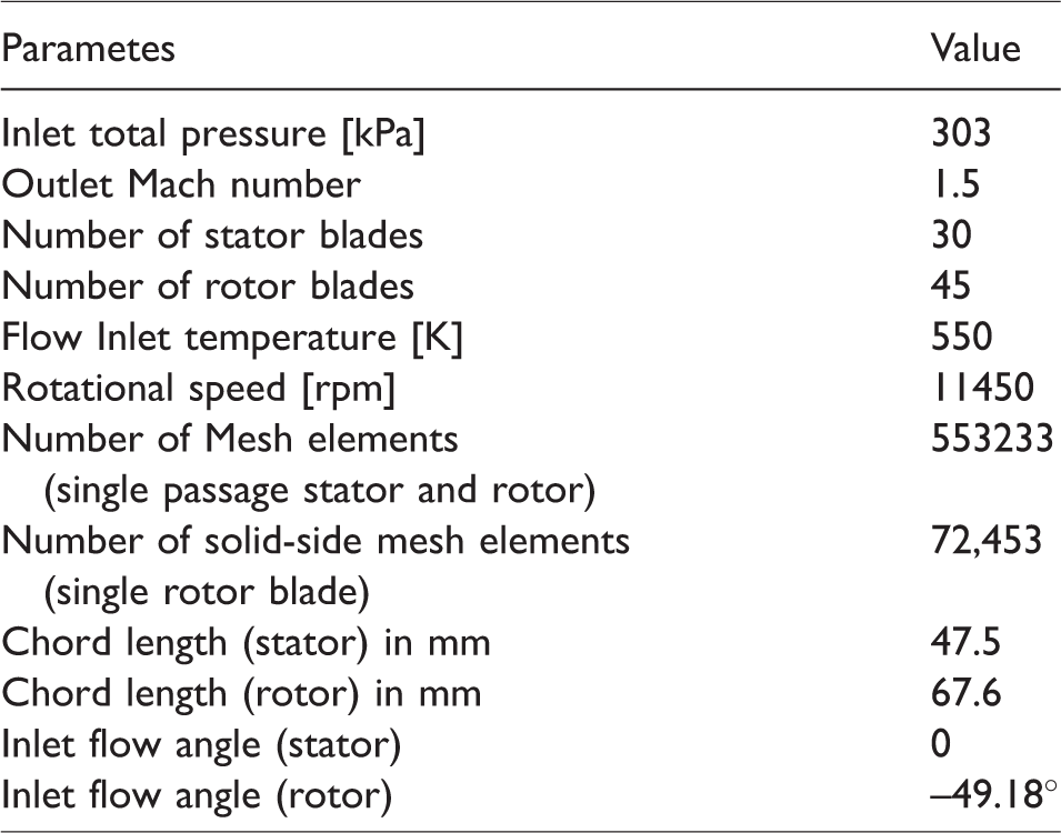
The test case considered for this numerical study is the turbine aerodynamic profile with experimental data obtained from Dunn et al. ²⁴ This is a stator-rotor configuration formulated to investigate the unsteady aerodynamics and heat transfer characteristics of a turbine stage. The operating conditions for the stage are shown in Table 1. The test case is a transonic flow model with oblique waves predicted at the stator-rotor blade row passage.

Table 1.

Vane blade Interaction (VBI) parameters.

Parametes	Value
Inlet total pressure [kPa]	303
Outlet Mach number	1.5
Number of stator blades	30
Number of rotor blades	45
Flow Inlet temperature [K]	550
Rotational speed [rpm]	11450
Number of Mesh elements (single passage stator and rotor)	553233
Number of solid-side mesh elements (single rotor blade)	72,453
Chord length (stator) in mm	47.5
Chord length (rotor) in mm	67.6
Inlet flow angle (stator)	0
Inlet flow angle (rotor)	–49.18°

The corresponding fluid domain meshes for the stator and rotor blades are shown in Figure 3. For picture clarity, the number of mesh points shown in the image is reduced from the actual points. A multi-block structures mesh was created using the ICEM CFD mesh package. An orthogonal grid arrangement was formulated near the blade wall surface for proper resolution of boundary layer flows to achieve a $y^{+}\sim 1$ . The flow state is marched in time until the solution residuals are below the set target of 1e-04. The converged solution state included a mass and energy balance checks at the inlet of the stator and rotor outlet.

Figure 3.

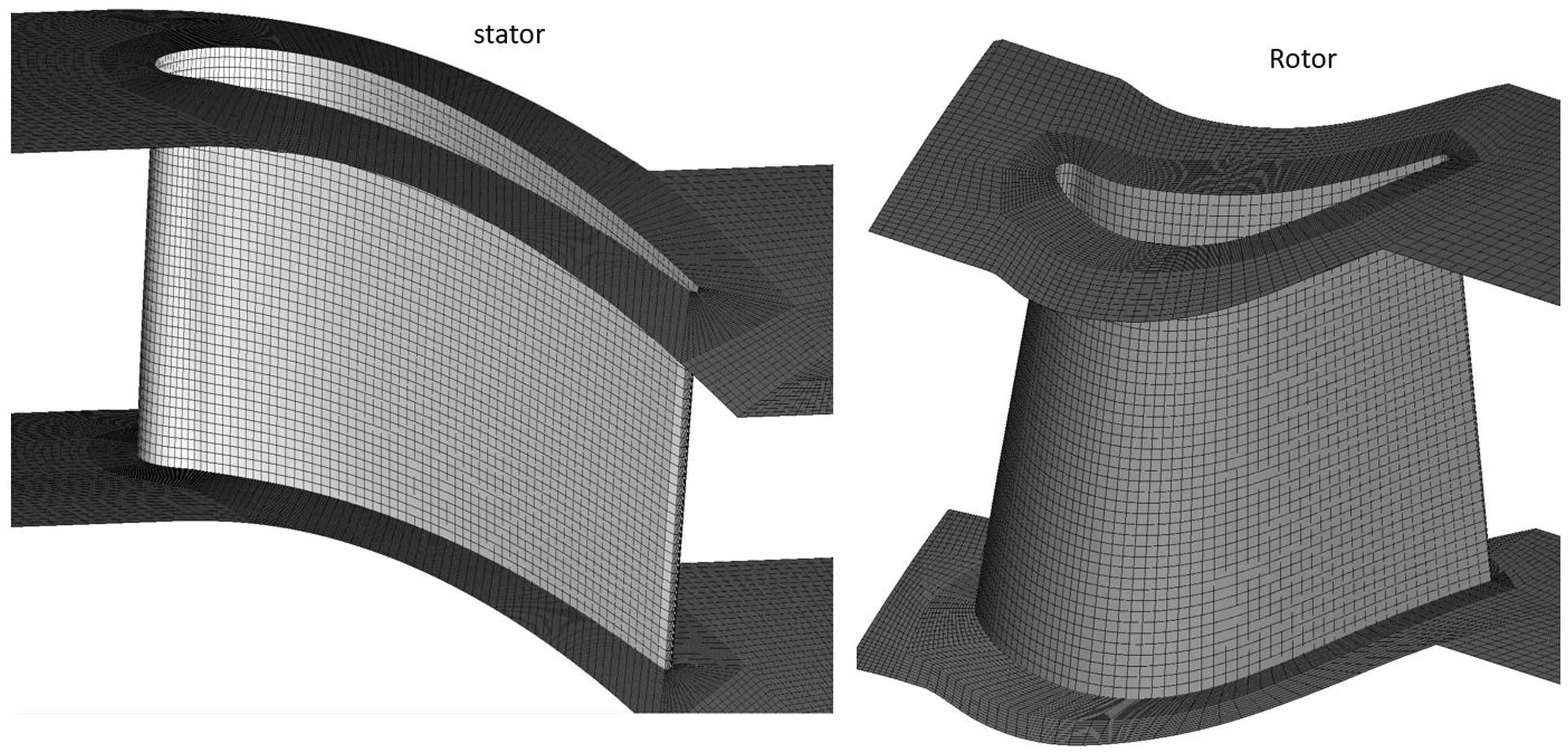
Stator and rotor blade mesh.

A mesh independent solution was used for the two simulation approaches and the final number of elements in the fluid and solid-side domains are shown in Table 1. This was obtained through a Grid convergence study by monitoring the area averaged quantity of the Turbulence Kinetic Energy (TKE) at the rotor outlet domain. The TKE measures the mean kinetic energy per unit mass of the flow unsteadiness.

Analytically, this was obtained through a measured root-mean square of the velocity fluctuations. The spatial convergence approach implemented follows the procedure outlined in Roache ²⁵ which is based on Richardson extrapolation. By using a mesh refinement factor of 1.5, starting from an initial mesh size of approximately 244,000 elements, the grid convergence index for the 3rd and 4th refinements was estimated as 0.91. By using the correlations presented in Slater, ²⁶ the estimated asymptotic convergence value of 0.66 was obtained for the 3rd mesh iteration of 553,233 elements. A value of asymptotic convergence value less than 1 indicates the solution are within the tolerance convergence limit. A fuller description of this grid convergence study was reported in previous publication by this author. ²⁷

Aerodynamic result

Figure 4 shows the velocity streamlines at 50% span position of the stator-rotor stage configuration. The direction of the rotor domain movement in relation to the stator domain is indicated by the arrow at the stator-rotor interface boundary. The order of the time plot is indicated by the numbering from 1∼4, representing the passing period as the rotor blade completely moves past a single stator passage. The rotor blades cross the wakes off the stator blade at periodic intervals determined by the reduced frequency and Strouhal number of the unsteadiness. For this configuration, the reduced frequency was estimated as 0.08, indicating a highly unsteady flow phenomenon, at a rotor chord length of 67 mm. Two specific regions of interest are marked with SB, indicating the formation of separation bubbles on the rotor pressure side and at the suction side of stator, near its trailing edge. As shown, the size of the bubble changes with the periodic movement of the rotor. At the third image, the blade has completed 1-stator pass and the formed separation zone moves upstream the blade passage. The reflected wave from the rotor passage also reduces the size of the separation in the stator domain, leading to early reattachment of the flow on the stator suction surface at the time where the rotor blade completes ½ of passing period. The accurate prediction of this unsteadiness is vital to the estimation of the vibrational forces and subsequent stress analysis

Figure 4.

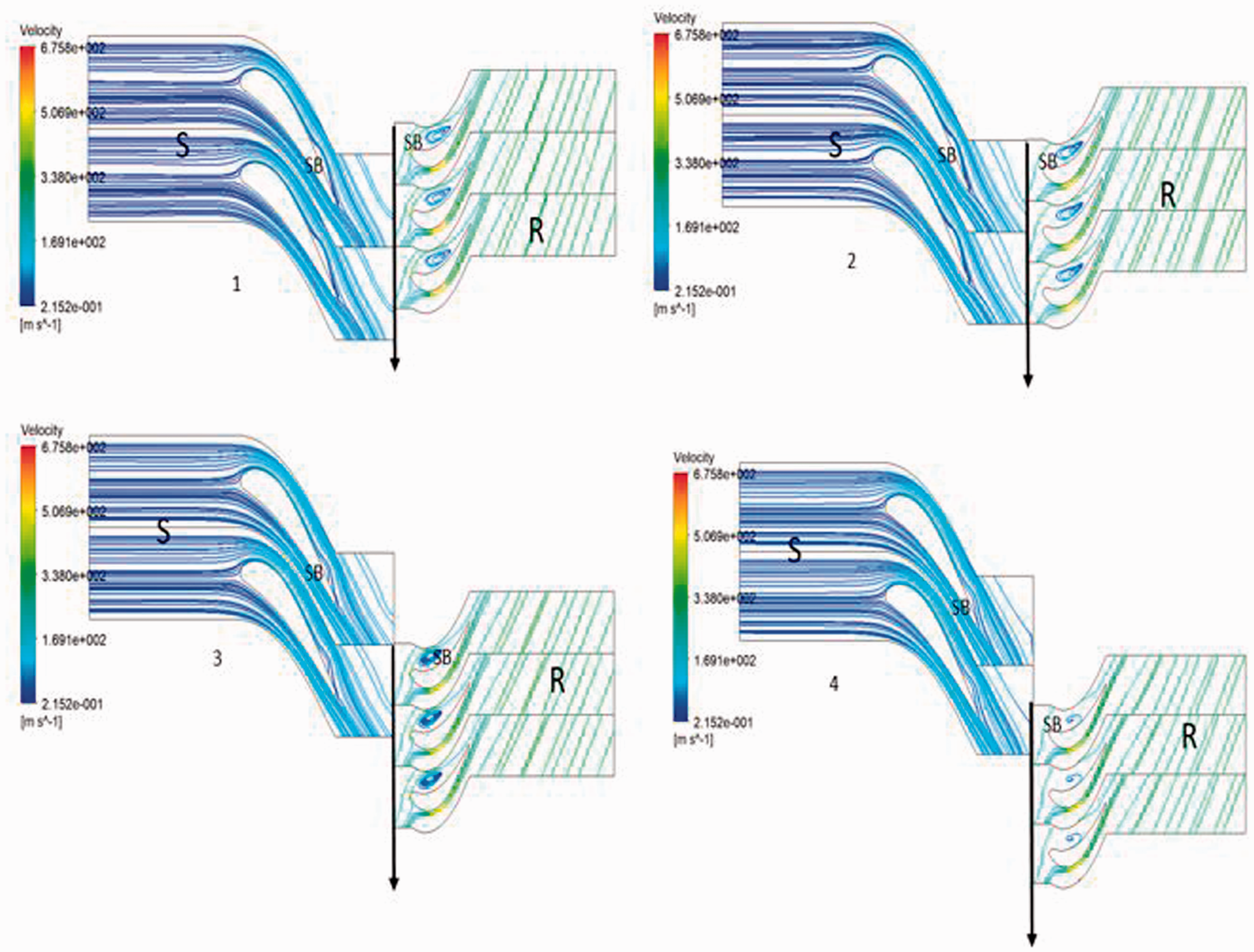
Velocity streamline plot at 50% span position.

Figure 5 shows the comparison of the coefficient of pressure estimation of this current study against the experimental data of Dunn et al. ²⁸ Also shown are the predicted non-dimensional heat transfer, Stanton number in comparison with experimental data. The unsteadiness in the suction surfaces of the rotor and stator blades is due to the noticeable oblique shock-wave in the passage. The shock-wave in the stator blade passage is an intra-blade row interaction case that is observed closed to the trailing edge between the suction and the pressure sides. These are convected downstream into the rotor domain, and with the high surface curvature of the of the rotor leading edge, resulted in a noticeable increase in the flow speed acting in addition to the domain axial velocity. The relative motion of the stator-rotor surface causes a periodically fluctuating flow, with significant unsteadiness in the pressure signals as shown in Figure 5. A similar stator-rotor interaction study on a closely spaced profile was reported in Allegret-Bourdon, ²⁹ where the presence of shock-waves in the flow-field showed a significant unsteadiness on the amplitude and the phase angle of the pressures values acting on the blade surface. This was also reported for this test case in the study by work Delaney et al. ³⁰

Figure 5.

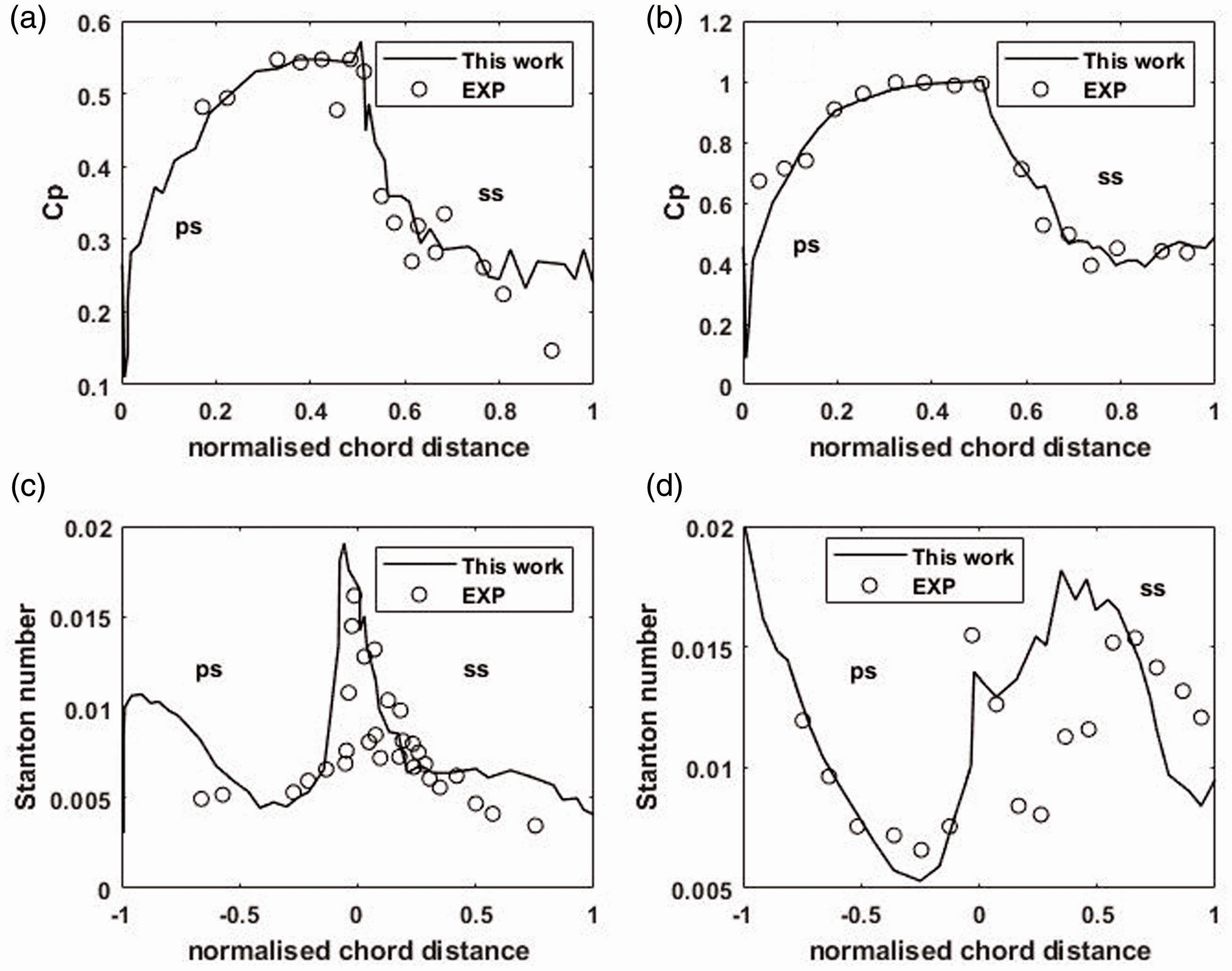
Pressure coefficient and heat transfer comparison with experimental data: (a) rotor blade coefficient of pressure, (b) stator blade coefficient of pressure, (c) stator blade heat transfer and (d) rotor blade heat transfer.

The above comparison serves to validate the solver capability in being able to predict the pressure distribution in relation to the experimental data. A fuller description of the flow field features was earlier reported in another report by this author. ²⁷

Results – transient response and stress profile

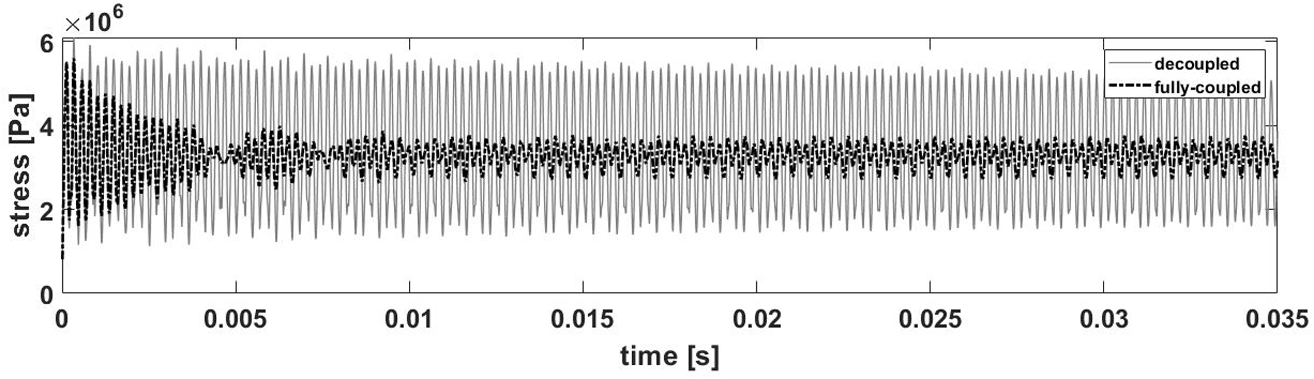
Figures 6 and 7 show the transient history of the maximum displacement and von Mises stress response at a node location of the rotor blade. For the von Mises stress case, the node location was at the root section on the suction side region of the blade. For the displacement history, the selected nodal point is the region of maximum displacement noticeable at the trailing edge near the 100% span location. These show the rotor blade response from the two simulation approaches with the decoupled case showing a higher amplitude of signal fluctuation than the prediction from the fully coupled method. This is shown for the low-cycle fatigue loading condition where the rotor blade is modelled taking into consideration the loading due to the high-rotational speed and the effect of unsteady pressure. The corresponding prediction depicting only the influence of pressure-only aerodynamic forces is shown in Figure 8. This also shows the overwhelming influence of the unsteady aerodynamic forces on the response history.

Figure 6.

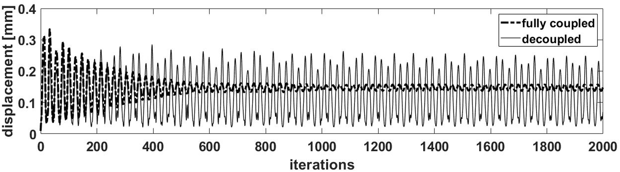
Displacement response for fully-coupled and decoupled solution approach.

Figure 7.

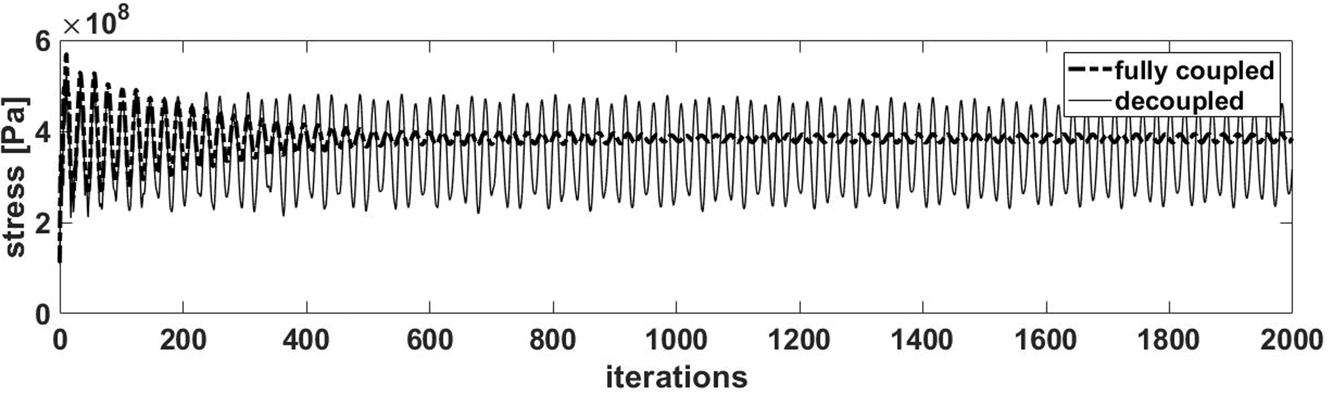
Stress history response for the fully-coupled and decoupled approach.

Figure 8.

Stress history from unsteady pressure loading.

The fully coupled case fluctuates with at a stress ratio $\mathrm{ }(R=\frac{{\sigma }_{\min }}{{\sigma }_{\max }}$ ) of 0.8 while the stress ratio of the decoupled approach is 0.5, with lower induced mean stresses. The material implemented in the finite element model is the steel alloy LC 304 material with yield stress of 250 MPa and an ultimate tensile strength of 460 MPa. For the fully coupled case stress history, the higher stress ratio (R) therefore depicts the presence of high mean stresses, which are largely due to the superimposed vibrational stresses of the unsteady pressure loading on the rotational load. Ideally, a stress ratio, R=–1 represents a fully reversed condition with low mean stresses induced. At the lower stress ratios, R∼0.1, the problem is mostly LCF dominant, depending on the amplitude of the induced mean stresses. Another relevant indicator of LCF or HCF failure mode was reported in Natchigall and Halford, ³¹ who used the parameter ( ${\Delta \epsilon }_p/{\Delta \epsilon }_e$ ) at the value = 0.1 to demarcate the point above which the mean stress effect should be considered. The presence of compressive mean stress is considered favorable for fatigue life improvement (as it enhances the fatigue life), while tensile mean stresses are more damaging and can lead to a significant reduction in fatigue life. In the case of the pressure-only stress response of Figure 8, the induced stresses are significantly below the material yield limit and as such, the ratio, $\mathrm{ }{\Delta \epsilon }_p/{\Delta \epsilon }_e$ is not able to give a true indication of the severity of the damage. However, in the loading profiles of Figure 7, the plastic-to-elastic strain ratio is above 0.2, indicating the need to consider mean stress effect in the fatigue life analyses. Boyce and Ritchie ³² investigated the influence of stress ratio on the fatigue threshold of an engine blade material. In using a fracture mechanics approach, it was shown that the high stress ratios resulted in a reduction in the threshold stress intensity factor and a faster crack growth rate for a given applied stress. This effect of stress ratio at near threshold levels was attributed to crack-closure phenomenon which is a characteristic of a roughness-induced mechanism on some turbine blade materials.

The 3 D contour plots of the displacement and stress distribution is shown in Figure 9. The maximum displacement is predicted at the tip of the blade for both cases of the decoupled or fully coupled method. This is at the trailing edge region of the blade due to the reduced material stiffness at this location. Similarly, the equivalent von Mises stress is radially distributed with a notch-like influence noticed at the root section of the suction side of the blade. This also shows the predominant load to be that of the centrifugal forces with a pulling effect in the radial direction. In both simulation approaches, the 3 D stress distribution on the rotor geometry were qualitatively similar, although the differing degree of the induced damage can only be closely observed in the monitored response history with noticeable differences in the amplitudes of fluctuation.

Figure 9.

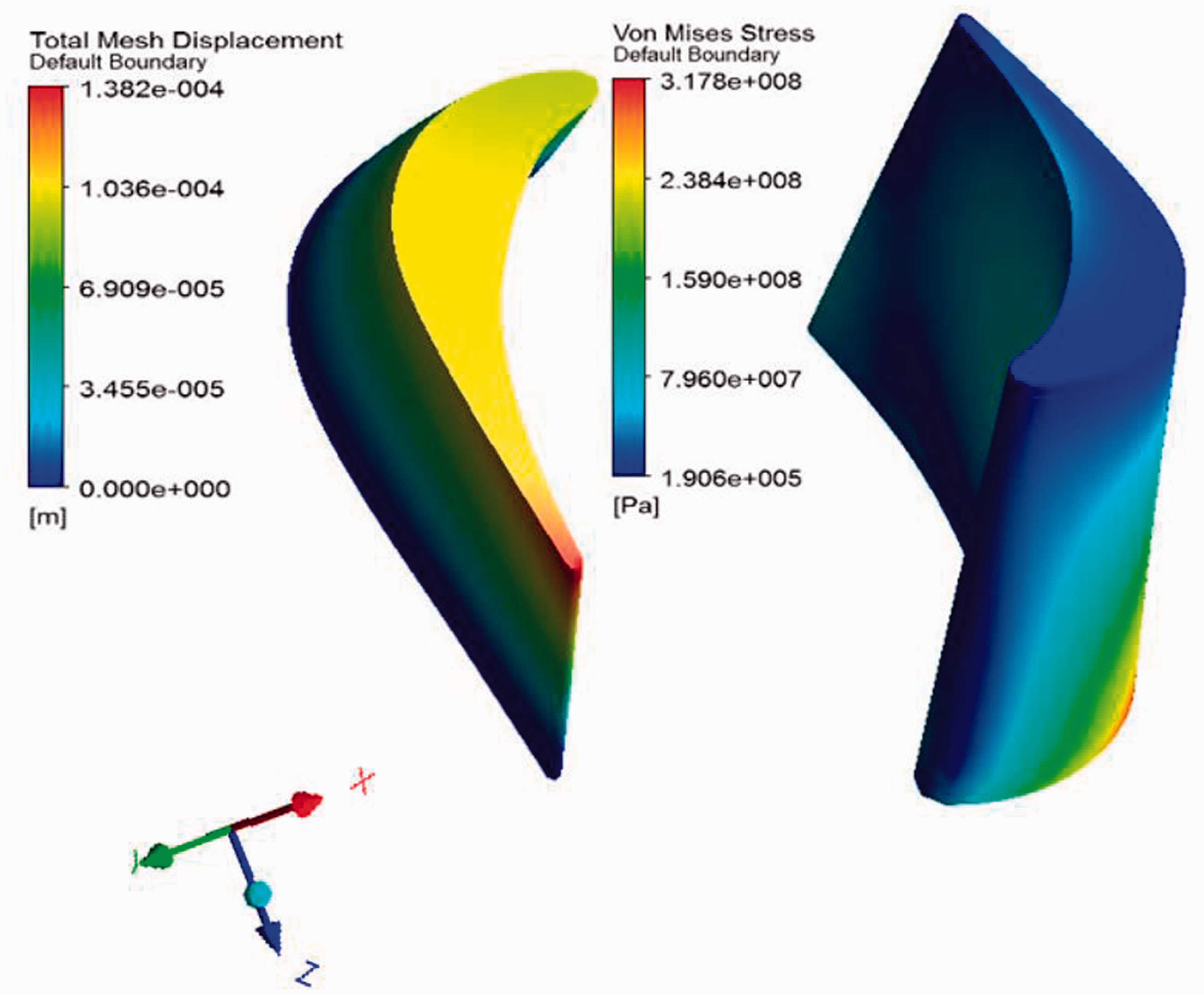
Displacement and stress contours for the rotor blade.

The transient computations were performed from an already established initial conditions using the solution output of a converged steady-state run. The high amplitude fluctuations noticeable in the predicted history at the start of the solution are due to transient scheme numeric. This arises from a two-fold effect of solver stability requirement and the added mass term of a fluid-structure coupling solution using a staggered iteration scheme. In the first case, the instability is an inherent property of the iterative solution approach of the implicit backward Euler method. As noted in literature,^23,33 the percentage period elongation and amplitude decays for this method can be quite large and can be dependent on the time step ratios. Secondly, it can be seen that the instability is dominant in the fully-coupled solution case. Given that the fully-coupled approach is implemented using a sequentially-staggered scheme rather than a monolithic approach, the associated instability is highly dependent on the solution timestep and this can be explained in light of the added mass effect of a fully-coupled scheme.^34,36 Due to the coupling framework, the fluid-forces are computed from the artificial interface displacement and this often leads to convergence difficulties and solution instability of the schemes. ³⁵ The added mass phenomenon is further explained in Section 5 of this work. However, despite these noted possibilities, the subsequent fatigue analyses only consider the converged solution state which is from the 1000th iteration step.

From the estimated stress history, the cycle counting algorithms of Irvine ³⁴ and Nieslony ³⁵ were used to extract the number of fatigue cycles. The algorithms allow for estimating half and full load cycles with amplitudes and mean values. Figure 10 shows the rainflow-extracted cycles for the fully coupled and decoupled stress histories of Figure 8. The fully coupled case shows the presence of high mean stress within the lower stress amplitude region, as compared to the decoupled case with high mean stresses within the high stress amplitude regions. Both cases show very little or sparsely distributed fatigue cycles which are typical characteristics of time domain analyses that often require a high-volume data in the rainflow cycle counting process. A similar distribution was noticed for the stress histories of Figure 7, however, with appreciable plasticity in the high stress region.

Figure 10.

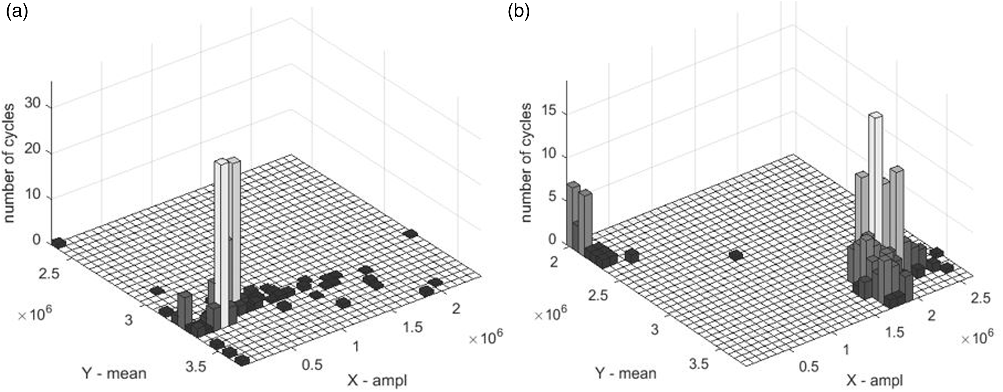
Rainflow matrix (a) fully coupled and (b) decoupled solution approach for pressure-only loads.

The multiaxial nature of the time history is represented by the 3 D Mohr circle representation of Figure 11. As shown, the blade response in both simulation approaches are predominantly biaxial. With the principal stresses $\left({\sigma }_1\ge {\sigma }_2\ge {\sigma }_3\right)$ arranged in decreasing order, the ratio of ${\sigma }_3$ to ${\sigma }_1$ is approximately 0.34 for both simulation approaches at simulation time t = 0.02s. The radius of the individual circles also indicates the amount of shear stresses present in the stress history, where the maximum radius is $0.5\left({\sigma }_1-{\sigma }_3\right)$ and the smallest radius as $0.5\left({\sigma }_2-{\sigma }_3\right)$ .

Figure 11.

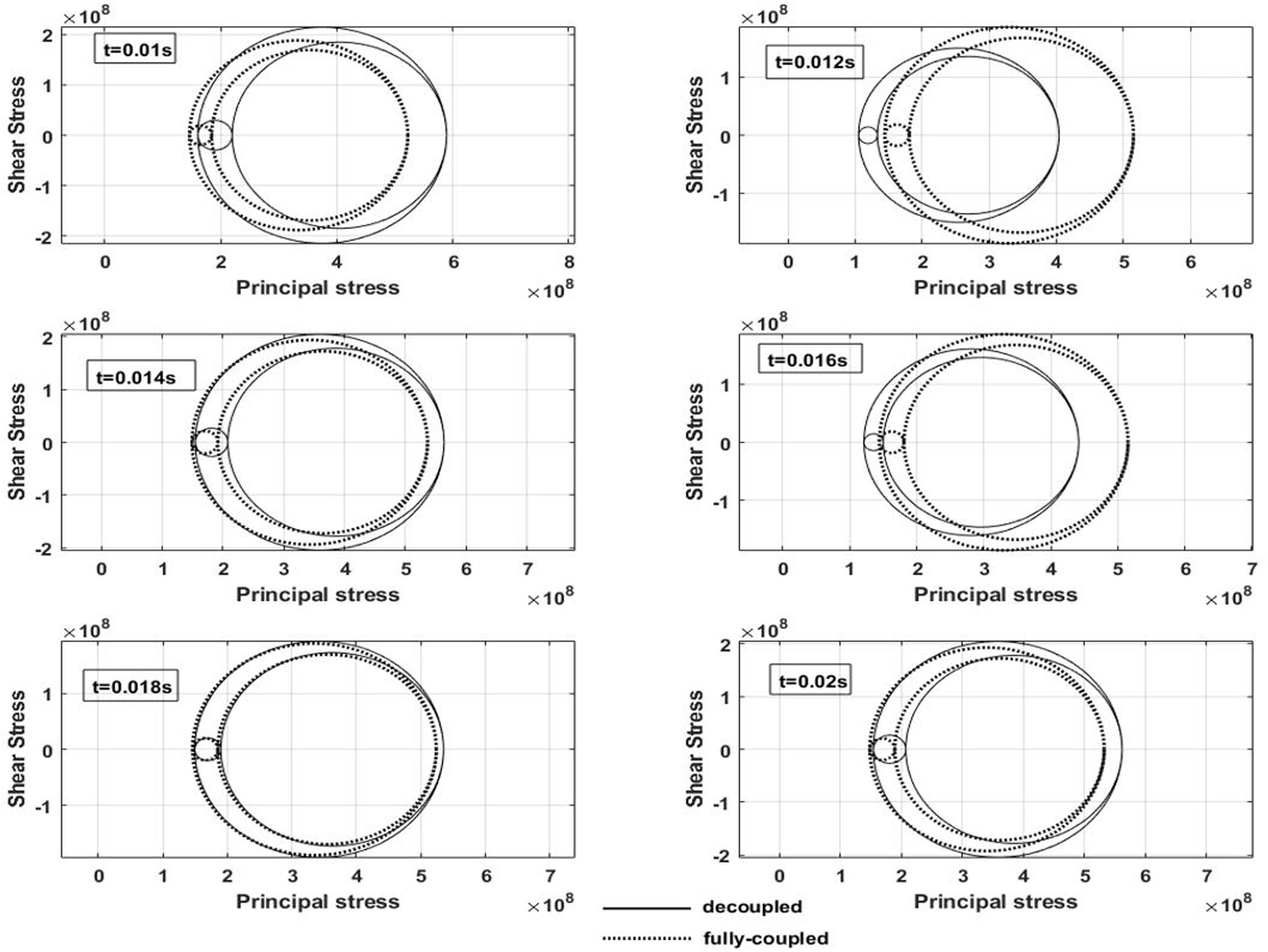
3D Mohr circle representation of time history stress data for the decoupled and full-coupled solution approaches.

Strain energy fatigue method

The fatigue analysis of the predicted stress histories is evaluated using the strain energy density method. The strain energy model is a relevant parameter for understanding the crack initiation and propagation phases of total fatigue life. By its definition, it enables the global and local material characterization, in both the low-cycle and high cycle fatigue regimes, to be related through the strain energy density parameter. The material’s fatigue resistance can be characterized by its capacity to absorb the input energy of a given cyclic load. The total strain energy is the sum of the elastic $\left(\Delta W^e\right)\mathrm{ }$ and the plastic $\left(\Delta W^p\right)\mathrm{ }$ energy, see Figure 12. The energy approach adopted for the fatigue life evaluation follows that of Kujawski and Ellyin, ³⁶ who presented this correlation using the plastic strain limit ( $\Delta {ϵ}_e^p$ ) from the cyclic stress/strain curve. The material fatigue limit, below which the energy parameter is insensitive to the damage threshold is related to the endurance stress range, $\Delta {\sigma }_e=K\mathrm{\prime }{\left(\Delta {ϵ}_e^p\right)}^{n^{\mathrm{\prime }}}$ , where $n^{\mathrm{\prime }}$ is the cyclic strain hardening exponent and $K\mathrm{\prime }$ is the fatigue strength coefficient. For most material, $\Delta {{\in }^p}_e$ is in the range ${10}^{-5}\sim \mathrm{ }5\mathrm{ }x\mathrm{ }{10}^{-4}$ . The cyclic hardening exponent $n^{\mathrm{\prime }}$ and the hardening coefficient $K\mathrm{\prime }$ were obtained through a curve-fitting procedure using a MATLAB optimization function by fitting a regression model to stress amplitude versus plastic strain data. The optimized parameters were obtained as 0.171 and 1338.4 MPa, respectively for $n^{\mathrm{\prime }}$ and $K\mathrm{\prime }$ .

Figure 12.

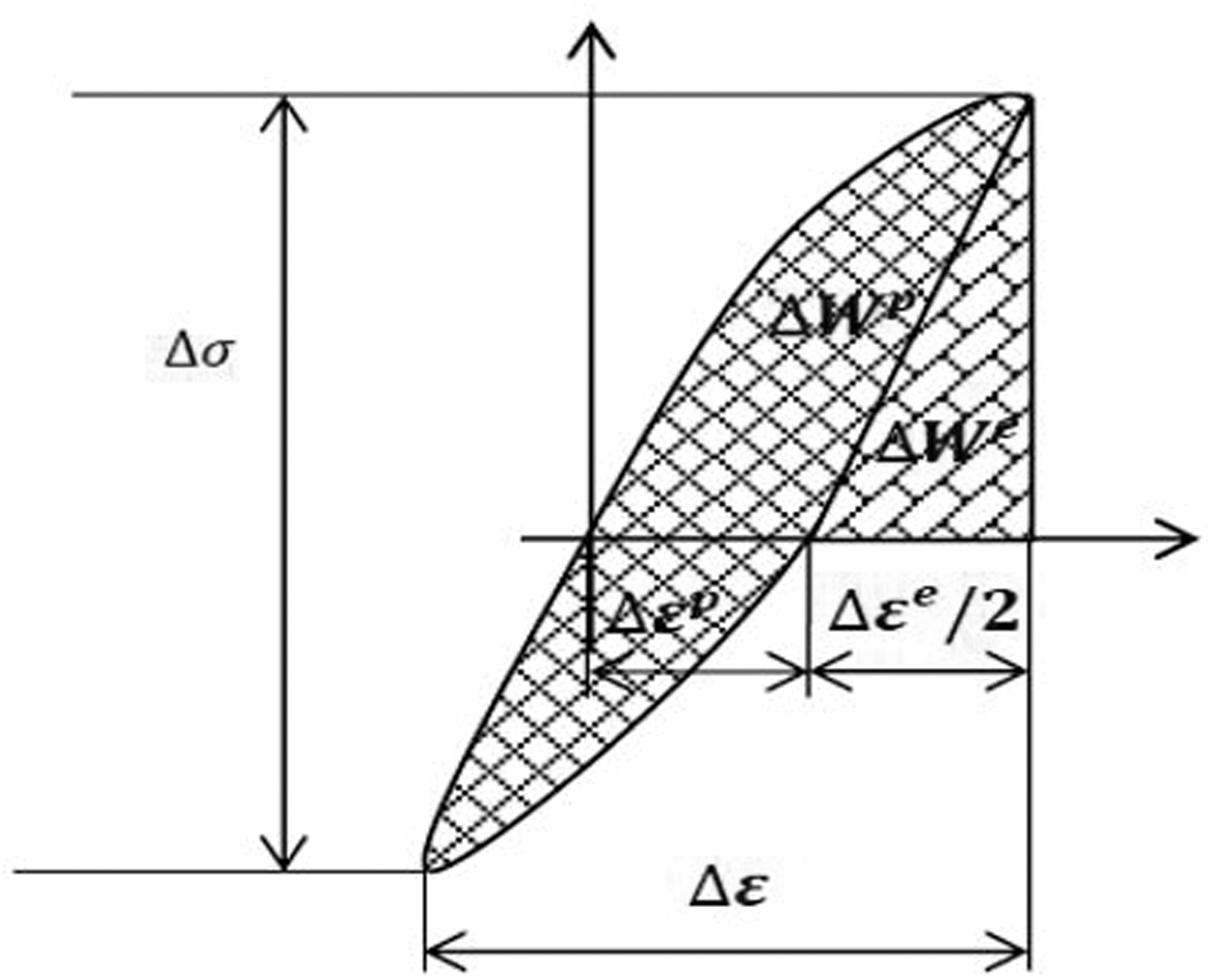
Strain energy decomposition of cyclic stress-strain loop.

From Figure 12, the total strain energy density can be represented in the form;

$${\Delta W}^{\mathit{total}}={\Delta W}^p+\Delta W^e$$

(12)

The terms on the RHS representing the plastic and elastic strain energy densities. This allows the plastic strain parameter to be formulated as the limit state condition during the crack initiation phase. The expression is related to the fatigue reversal cycles in the form;

$$\Delta W^{\mathit{total}}=k{\left(2N_f\right)}^a+{\Delta W}_{\mathit{end}}$$

(13)

Where $k$ is the energy at the intersection of the straight line with the slope $\alpha$ on the energy axis. The parameters were obtained using the same least square regression technique on a material data of strain energy density per cycle versus number of cycles to failure data as per Ellyin and Kujawski. ³⁷ The corresponding data for Inconel type alloys can be found in Glinka et al. ³⁸ The obtained best fit values were 1375 MJ/m³ and –0.58, respectively for $k$ and $\alpha$ . A known limitation of $\Delta W^p$ parameter can be that it is insensitive to hydrostatic pressure stresses and the associated difficulty in measuring the plastic strain energy near the material fatigue limit, which for most metals is within the range 10⁻⁵ to 5 × 10⁻⁵. For a positive hydrostatic stress, the induced fatigue damage is observed at a higher rate as this directly contribute to crack opening. Similarly, for compressive hydrostatic stresses, the crack tip is blunted leading to a crack closure phenomenon with a resultant reduction in induced damage. This effect has led to the postulation that compressive stresses are favorable to enhance fatigue resistance of certain materials McDiarmid. ³⁹ Given these setbacks, a way to address this is therefore to formulate the cyclic life using the total strain energy parameter as shown in Equation 12. The respective relations for the elastic ${(\Delta W}^e)\mathrm{ }$ and plastic energy $\left({\Delta W}^p\right)$ density terms are therefore estimated as;

$${\Delta W}^e=\frac{1}{2E}{\left(\frac{\Delta {\sigma }_r}{2}+{\sigma }_{\mathit{mean}}\right)}^2$$

(14)

$${\Delta W}^p=\frac{1-n^{+}}{1+n^{+}}\left({\Delta \sigma }_r-{\delta \sigma }_0\right){\Delta \epsilon }^{\mathit{plastic}}+\delta {\sigma }_0{\Delta \epsilon }^{\mathit{plastic}}$$

(15)

$${\delta \sigma }_0=\mathrm{ }{\Delta \sigma }_r-2E_0^{+}{\left(\frac{1}{2}{\Delta \epsilon }^{\mathit{plastic}}\right)}^{n+}$$

(16)

$${\Delta W}_{\mathit{end}}=\frac{1}{2}\frac{\Delta {\sigma }_e}{2}\frac{\Delta {\epsilon }_e^{\mathit{elastic}}}{2}$$

(17)

Where ${\Delta W}_{\mathit{end}}$ is the strain energy at the material endurance limit that does not contribute to damage, and ${\Delta \sigma }_r$ is the predicted stress range. ${\delta \sigma }_0$ is the proportional stress limit, which is an indication of the Masing or non-Masing material behavior. In Equation 14, the elastic strain energy density term takes into account the mean stress effect. ⁴⁰

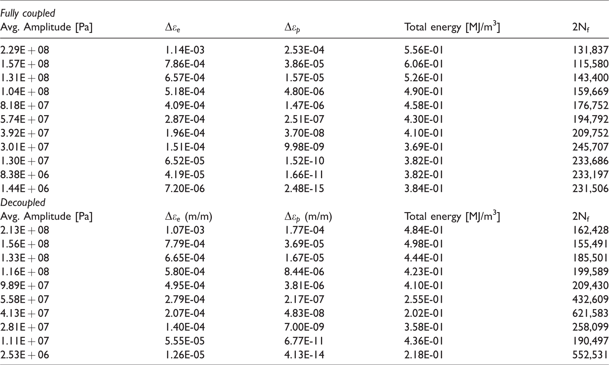
From the estimated LCF-HCF stress history of Figure 7, Table 2 shows the estimated fatigue lives using the strain energy density equations. As shown, the fatigue life is primarily determined by the combined elastic and plastic strain components. While the bulk material response might be elastic, at microscopic grain level significant plastic deformation may occur. Reported experimental observations have shown that for loadings slightly below the material fatigue stress limit, it is possible to notice microcracks and persistent slip bands of the range 10⁻⁵ – 10⁻⁴ m at the microscopic level. This resulted in a fatigue threshold stress intensity factor for this material as 3 MPa $\sqrt{m}$ as was earlier reported in Ubulom et al. ⁴¹ Table 2 therefore shows the estimated fatigue reversal cycles for the decoupled and fully-coupled stress. The least predicted fatigue cycles for the fully-coupled method was 132,000 cycles, while that of the decoupled method was 162,000 cycles. For both cases, the induced elastic energy density was estimated higher than the plastic energy at the limiting condition, depicting that the bulk of the failure is HCF dominant.

Table 2.

Fatigue life estimated from the strain energy density method.

Fully coupled
Avg. Amplitude [Pa]	${\mathrm{\Delta }\epsilon }_e$	${\mathrm{\Delta }\epsilon }_p$	Total energy [MJ/m3]	2Nf
2.29E + 08	1.14E-03	2.53E-04	5.56E-01	131,837
1.57E + 08	7.86E-04	3.86E-05	6.06E-01	115,580
1.31E + 08	6.57E-04	1.57E-05	5.26E-01	143,400
1.04E + 08	5.18E-04	4.80E-06	4.90E-01	159,669
8.18E + 07	4.09E-04	1.47E-06	4.58E-01	176,752
5.74E + 07	2.87E-04	2.51E-07	4.30E-01	194,792
3.92E + 07	1.96E-04	3.70E-08	4.10E-01	209,752
3.01E + 07	1.51E-04	9.98E-09	3.69E-01	245,707
1.30E + 07	6.52E-05	1.52E-10	3.82E-01	233,686
8.38E + 06	4.19E-05	1.66E-11	3.82E-01	233,197
1.44E + 06	7.20E-06	2.48E-15	3.84E-01	231,506
Decoupled
Avg. Amplitude [Pa]	${\mathrm{\Delta }\epsilon }_e$ (m/m)	${\mathrm{\Delta }\epsilon }_p$ (m/m)	Total energy [MJ/m3]	2Nf
2.13E + 08	1.07E-03	1.77E-04	4.84E-01	162,428
1.56E + 08	7.79E-04	3.69E-05	4.98E-01	155,491
1.33E + 08	6.65E-04	1.67E-05	4.44E-01	185,501
1.16E + 08	5.80E-04	8.44E-06	4.23E-01	199,589
9.89E + 07	4.95E-04	3.81E-06	4.10E-01	209,430
5.58E + 07	2.79E-04	2.17E-07	2.55E-01	432,609
4.13E + 07	2.07E-04	4.83E-08	2.02E-01	621,583
2.81E + 07	1.40E-04	7.00E-09	3.58E-01	258,099
1.11E + 07	5.55E-05	6.77E-11	4.36E-01	190,497
2.53E + 06	1.26E-05	4.13E-14	2.18E-01	552,531

The choice of the strain energy method was precipitated upon the fact that the chosen model can account for HCF -associated phenomenon of elastic strain, while also being to account for the LCF influence due to the inelastic strain ranges. As it is the case with most fatigue life prediction, a review of several fatigue models by Zhuang and Swansson ⁴² showed that most of the available fatigue models are only able to predict the fatigue life with acceptable accuracy within a certain material envelope and test condition. However, no model has been shown to satisfactorily predict fatigue life with exceptional accuracy for all materials under varying service conditions. A similar conclusion on the prediction accuracy and wide acceptability of various fatigue models was reported in a recent review by Santecchia et al. ⁴³ The selected model as used in this study is one of the limited approaches that have shown robustness and formulated based on the physical principle of HCF and LCF failure conditions and has been validated for this material and expected environmental condition.^44,45

However, given the highly stochastic nature of the predicted loading profile, a statistical evaluation of the above predicted fatigue lives is useful to reduce conservativism in the process and to quantify the relevant drivers from the two simulation approaches. The challenge, however, lies in formulating an appropriate stochastic model that will accurately describe the randomness of the induced loading and material properties. A recent application of the strain energy density method for fatigue failure of metals had shown the predicted lives to follow a lognormal distribution. ⁴⁶ Therefore, based on the assumption of the renewal process and for a cumulative damage summation case, the mean and standard deviation of the input data was established following the method proposed in Tiiu and Bienek ⁴⁷ as;

$${\mu }_D=\sum _i\frac{{\mu }_{n_i}}{{\mu }_{N_i}}$$

(18)

$${{\sigma }^2}_D=\sum _i\frac{{(\mu }_{n_i})\mathit{Var}\left(N_i\right)}{{\mu }^3\left(N_i\right)}+\mathit{Var}\left[\sum _i\frac{n_i}{\mu \left(N_i\right)}\right]$$

(19)

The formulated lognormal approach was adopted to understand the inherent stochastic properties of the response signals. For example, the load history effect was estimated from the counted applied cycles and assumed to be a random variable with mean and variance. The damage function distribution is therefore defined assuming a log-normal distribution of the form;

$$P\left(D\ge 1\right)=\mathrm{\Phi }\left(-\eta \right)=\frac{1}{\sqrt{2\pi }}{\int }_{\eta }^{\mathrm{\infty }}{e}^{-\frac{y^2}{2}}\text{d}y$$

(20)

$$\eta =\frac{-\left[\ln \left({\mu }_D\right)-\ln \left(\sqrt{1+V_D^2}\right)\right]}{\sqrt{\ln \left(1+V_D^2\right)}}$$

(21)

In the relations above, $\mathrm{ }{\mu }_D,V_D$ are the mean and coefficient of variation of the random variable $y.$ The higher the coeffiient of variation, the higher the scatter in the damage variable and as such, the standard deviation of the process. Other recent studies adopting a similar approach for reliability estimation are based on the mean and the standard deviation parameters of the random variable for turbine material.^48,49 By fitting a relationship to their obtained relaibility data, a correlation was drawn between the service life and the dispersion of random loads based on the coefficient of deviation. The coefficient of variation herein representing the ratio of the standard deviation to the mean value of the random vector. This enables the statistical assessment of the design variability, in terms of stress, energy density and other fatigue variables. In a prior report of the current work, the weighting distribution for the various fatigue random variables were analysed using the probability sensitivity factor. This gives a rank of the order of random variables on the probability of failure of engineering components. This was demonstrated by ranking several variables including the counted rainflow cycles, stress amplitude and the S-N fatigue cycles. Interested readers can see Ubulom. ²⁷

Figure 13 shows the probability densities for the fatigue parameters of the two simulation approaches. The stress amplitude, energy density and fatigue cycles are lognormally distributed and were obtained from a Markov-chain Monte Carlo sampling of the data in Table 2. The figure also shows the probability distribution for the fatigue facture plane in terms of the direction of the principal stresses from the 3D Mohr circle representation of Figure 11. Given the non-positive orientation of the angles for the transformed stress state, the Euler angles were sampled using the normal distribution.

Figure 13.

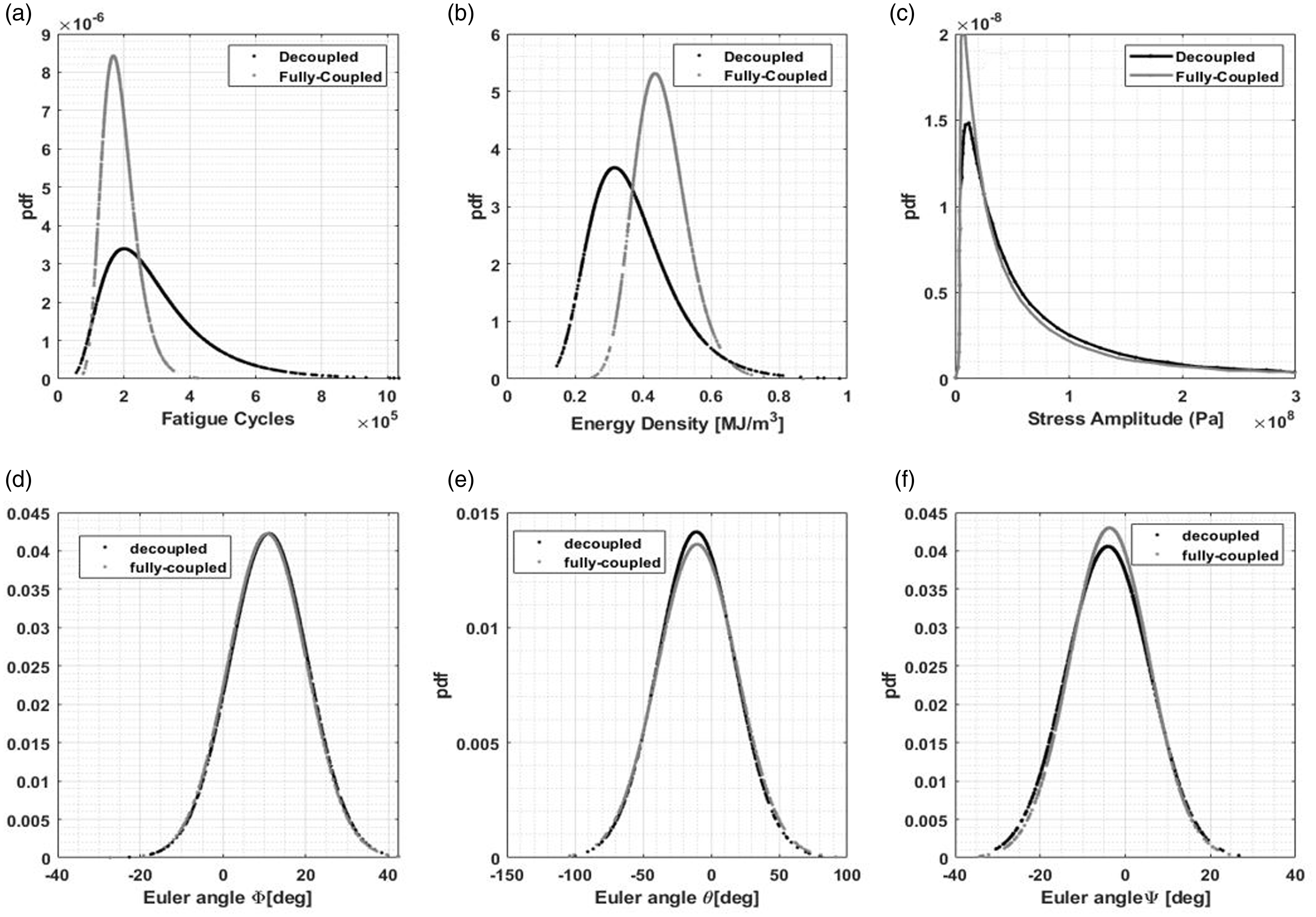
Probability densities of (a) fatigue cycles, (b) strain energy density, (c) mean stress, (d) Euler angle 1, (e) Euler angle 2, (f) Euler angle 3 for the fully-coupled and decoupled solution approaches.

Discussion

In the fatigue analysis presented in Table 2, it is seen that the predicted fatigue lives are predominantly influenced by the magnitude of the elastic strain energy. The plastic energy density was also found to be higher for the fully-coupled case than the decoupled solution approach. As shown, the limiting fatigue life for the fully-coupled is predicted at 132,000 cycles, as compared to 162,000 cycles for the decoupled approach. The elastic strain energy which is dominant in the high-cycle fatigue region was also higher for the fully-coupled. The lower fatigue life of the fully-coupled approach can be attributable to the higher stress amplitude and mean stress present in the history profile. This is evident in the probability distribution plot where the distribution is centered around 380MPa for the fully-coupled case as compared to the mean value of 350MPa for the decoupled case. In both approaches, the high mean stress values are mainly due to the high rotational velocity of the rotor wheel, where the influence of unsteady pressure loads, although mainly elastic nature as shown in Figure 8, contain some excitation frequencies near the third blade mode of combined bending and torsion. The visible differences in the stress responses are shown in Figures 7 and 8. Although the fluctuations in the fully-coupled case are highly damped, the mean distribution is significantly higher than the decoupled history.

This additional damping of the fully-coupled method was previously explained as an added mass parameter in Liu. ⁵⁰ The added mass was considered as a region of fluid attached to the moving boundary which adds to the total inertia force of the body. In a compressible flow case, the added mass term is proportional to the length of the time interval, ⁵¹ while for an incompressible flow case, it can yield unstable computations and highly dependent on the mass density ratios of the fluid to solid domains. ⁵² An extensive consideration of this effect in the context of a fluid-structure coupled analysis was given in Liu and O’Farrell. ⁵³ As modelled in the current study, the turbine blade profile analyzed experiences all the four broad categorizations of the fluctuating fluid forces; including extraneously induced excitation from the boundary layer build-up around the blade and turbulent nature of the flow, upstream stator instability forces, rotational domain boundary forces and excitation from the fluid oscillation due to three-dimensional flow features. The added mass parameter due to the movement induced forces can either be induced in-phase or out-of-phase with the blade displacement. In a coupled simulation case, these fluid forces can act as an added mass and as damping forces. In a study reported in Moffat and He, ⁵⁴ a reduction in the vibration amplitude was noticed in the coupled simulation approach and was attributed to the added mass effect. As opposed to the initial assumption of the added mass effect as due to a region of fluid attached to a moving solid boundary, it was shown in Moffat and He ⁵⁴ that this was not the case of a turbomachinery blade which is characterized by very thin boundary-layer regions of low-density fluid.

The reduction in the predicted response as compared to the decoupled approach was however, explained as an in-phase component of the aerodynamic force which exhibits an energy-dissipating influence in the fully-coupled method. As shown in the current analyses, the inertial component of the aerodynamic force acts in addition to the inherent material damping to lower the mean response amplitude for the fully-coupled case, the turbine blade is mostly in an aeroelastic stable condition with no region of instability such as flutter noticed as observed from the work coefficient analysis of the various stress histories. This observation was drawn by evaluating the sign of the aerodynamic work coefficient, which is defined as the normalized work done by the unsteady pressure on the blade for each cycle of oscillation. Thus, a negative work coefficient is an energy dissipative with the blade transferring energy to the flow. On the other hand, the transfer of the energy from the flow to the blade results in a positive work coefficient for a stable condition. In the analyses above, although a low amplitude normalized coefficient was predicted, the sign value of the work coefficient was positive for all the coupling approaches, with higher magnitude in the fully-coupled case. Here, the vibration of the blade induces a local unsteady pressure field in the flow domain with a resulting aerodynamic damping that is higher in the fully-coupled case. Another point to note in the formulation of the decoupled approach is the assumption that the structural mode shapes are not affected by the aerodynamic forces. This is generally upheld to be valid for turbomachinery blades characterized by high stiffness and high-density profiles that often vibrate at very low amplitudes. However, as shown in the predicted blade responses of the current work, the fully-coupled approach taking into account the feedback influence between the fluid and solid equation fields, predicts an additional damping force which further reduces the response amplitude in comparison to the decoupled approach. Therefore, this shows the breakdown of such assumptions in the current case of a transonic flow field. A similar observation was made in Ubulom, ⁵⁵ where it was reported that such assumptions can only hold at the onset of flutter and would likely break down for lightly damped profiles, and also under a transonic flow condition where even a seemingly small oscillation can lead to nonlinear behavior. Furthermore in Moffat and He, ⁵⁴ this additional damping force was predicted to lag the blade motion in a typical forced-response vibration case. Through a Fourier decomposition of the damping force, the extra damping from the fully-coupled approach was shown to be provided by the imaginary (out-of-phase) component of the added mass term, while the imaginary part was aligned with the blade inertial force leading to a change in the dynamic mass. This added mass effect was therefore responsible for the change in the blade dynamic resonant frequency.

Noting this variation, the predicted stress histories of the two approaches were further analyzed to understand its influence on the multiaxial stress state of the blade. This is represented in 3 D Mohr circle representation of Figure 11. This also shows the time evolution of the transient stress state thereby depicting the magnitude of the principal and shear stress magnitudes. It can be inferred from the figure that for both simulation approaches, the loading state is predominantly in the blade tangential direction, where the ratio of $\frac{{\sigma }_1}{{\sigma }_2}$ ∼3 for both approaches in the converged solution state at 0.02 s. Correspondingly, a shear stress magnitude of about 190 MPa was predicted for the fully-coupled case and approximately 170 MPa for the decoupled solution case at simulation time $t=0.02s.\mathrm{ }$ A multiaxial stress state was noticeable with a significant amount of shear stress in the principal direction. For the typical ductile material under consideration, it is known that the plane of fracture is that of the maximum shear. These are also the planes of fatigue crack initiation due to the intensified slip process on the crystallographic planes. The predominant loading force is the tangential pull force inducing tension in the blade. In a classical mode I of crack growth process, it is well established that the slip processes and decohesion in front of the crack are mainly shear plane driven. ⁵⁵ Similarly, in a stage II of crack growth process, although the dislocation mobility is controlled by the tensile strain present, the slip and decohesion process is also shear dependent. From a separate analysis of the above predicted stress histories, the shear stress histories were similar to that of the equivalent von Mises case of Figure 13, with the fully coupled case fluctuating about the mean position of the decoupled case. This high amplitude of shear stresses indicates the presence of a complex multiaxial stress state, which is outside the scope of simpler analysis methods such as the Goodman diagram that is mostly applicable to uniaxial fatigue data. ⁴⁴ It is an insufficient means of adjudging the proper fatigue condition with a multiaxial stress state. Such complex stress state as predicted in this case, is difficult to replicate under a typical laboratory condition. As noted in Scott-Emuakpor et al., ⁴⁵ the difficulty lies in the significant amount of time required to obtained realistic high-cycle data, even under a uniaxial test condition. As shown above, by adopting the strain energy density approach for the LCF-HCF life estimation, the method is able to characterizes a material loading where a portion of the applied mechanical energy contributes to the damage while the remaining is exhausted in form of residual heat.

In Figure 13 are the distributions of the three Euler angles from the two simulation methods. These show the distribution of the expected principal stress direction in relation to the fatigue fracture plane. The Euler angles were obtained through an instantaneous averaging procedure with the use of suitable weight functions proposed by Carpinteri et al. ⁵⁶ The weight functions are determined as a parameter of the S-N curve and the fatigue stress limit of the material. At each time instant, a 3 x 3 matrix of the stress tensor was obtained, and an averaging procedure was adopted to eliminate the orthogonal matrix that will result from selecting only 3-of-9 components of the matrix. The three principal stresses are the eigenvalues of the stress tensor matrix and the eigenvectors represent the principal direction cosines. Judging by the degree of multiaxiality of the predicted stress state, these values therefore indicate the degree of rotation of the principal stress direction. The Euler angles $\mathrm{\Phi },\theta ,\mathrm{\Psi },$ represent the orientation of the principal stresses $\left({\sigma }_1\ge {\sigma }_2\ge {\sigma }_3\right)$ in the counterclockwise rotation of the XYZ in three-dimensional space. The current orientation of the axes can be seen in the contour representation of the 3 D stress and displacement of the rotor blade in Figure 9. From the probability distribution of Figure 13, the three principal Euler angles of the two simulation approaches vary simultaneously with little variation in the peak of distribution. The averaging procedure adopted for decomposing the angles are restricted to the range $-\frac{\pi }{2}\le \psi ,\theta ,\varphi \le \frac{\pi }{2}$ . As shown, the degree of orientation of the principal stress angles depicts a non-proportional loading behavior which can induce more fatigue cracks as compared to a proportional loading case. It is known that a complex rotation of the principal stress direction as shown in the case above can lead to the activation of the slip bands in the material grains. ⁵⁷ The position of the critical plane would be influenced by the directions of the maximum principal stress. In the current case where the mean stresses (Figure 13(c)) are high in comparison to the to the variable stress amplitudes, it is likely that the position of the critical plane would approach the plane of the maximum principal stresses. A similar dominant influence of the high mean stress was reported in relation to the crack initiation phase for smooth specimens. ⁵⁸ Its corresponding influence in the propagation phase, however, is dependent on the prior occurrence of intergranular fracture.

Lastly, it should be mentioned that the predicted stress profile of Figure 7 reveals the fluctuation at varying stress ratios, R, for both the fully-coupled and decoupled approaches. A similar trend is also noticed in the unsteady pressure induced stresses of Figure 8. The fully-coupled simulation predict a stress ratio R $\sim \mathrm{ }0.8,\mathrm{ }$ while the decoupled stress history fluctuates at a lower stress ratio of 0.4. The higher stress ratio of the fully coupled case also confirms the presence of high mean stresses in the signal. At high mean stresses (high-stress ratio), previous studies have shown that the fracture mode would likely change from a rate dependent failure mode to that of combined rate and time-dependent plasticity failure. ⁵⁹ From a crack propagation study, ³² showed that high load ratios result in a lower ${\Delta K}_{th}$ with faster crack growth rate at a particular stress intensity factor. Also, at R∼0.5, the parameter ${\Delta K}_{th}$ is found to be independent of the stress ratio. Morrissey et al. ⁶⁰ investigated the influence of test frequency on a compressor blade material at various stress ratios. Thus, at low stress ratios, the fatigue strength increases with increasing frequency. With the increasing stress ratios, the effect of frequency becomes irrelevant, at the point the material behavior is predominantly that of void nucleation and growth with no corresponding crack initiation or growth evident for the low stress ratio ranges. From the estimated fatigue live, the higher stress ratio of the fully-coupled is responsible for the reduced life to crack initiation by approximately 30,000 cycles lower than that of the decoupled method. In a study by Evans et al., ⁶¹ this effect of high stress ratio in reducing the number of cycles to crack initiation was attributable to two eminent factors; the increase in the rate of propagation and the reduction of critical fatigue crack size.

Conclusion

The stress and fatigue properties of a turbine blade are analyzed by comparing the response from two simulation approaches of a fully-coupled and decoupled simulation approach. In the fully coupled method, the solutions of the compressible fluid flow model and the solid nonlinear finite element models are obtained concurrently with a message passing interface implemented for exchanging solution variables between the two solvers for each advected time solution. In the second method of decoupled analyses, the fluid-only flow fields are initially predicted, and the unsteady pressure are unilaterally transferred to the finite element solver as boundary conditions. The comparison between the two simulation methods are drawn considering the nodal stress and fatigue responses. From the fatigue analysis of the two methods using the strain energy density approach, the following conclusions can be made from this study;

The fully-coupled case showing the effect of fluid-solid interaction predicted a higher mean stress than the decoupled approach.

The added mass effect noticeable in the predicted stress history of the fully-coupled is responsible for the initial solution instability of the staggered solution scheme with a resultant reduction in the fluctuation stress amplitude as compared to the decoupled approach.

The presence of the higher mean stress in the fully coupled method also resulted in a reduced fatigue life by approximately 30,000 cycles to crack initiation, in comparison to the decoupled approach.

This was also evident by the higher fluctuating stress ratio of the fully-coupled which is a relevant parameter in the crack propagation phase.

In both simulation approaches, a strong multiaxial stress state was predicted, with a slightly higher shear stress amplitude in the fully-coupled case.

The orientations of the stress responses were also examined based on the Euler angle evaluation. Although the probability density distribution of both approaches showed very little differences, the rotation of the direction of the principal stresses over a wide angle also confirms the presence of a strong multiaxial stress state on the turbine blade.

Finally, while previous assumptions in support to the decoupled approach holds that due to the high mass ratio of the high-pressure turbine blade to the fluid density that there is negligible influence of blade displacement on the aerodynamic response and vice versa, the current analyses have shown that even for moderately stiff profile, the influence of the coupled interaction can lead to changes in the fatigue properties and life evaluation of a turbomachinery blade.