Sage Journals: Discover world-class research

Abstract

This research examines the interactions between fracture depth and crack location on a cantilever beam’s dynamic response under thermomechanical loads. The structure’s stiffness is significantly influenced by temperature, and changes in stiffness can alter the response’s damping, frequency, and amplitude. The basis for measuring damage to an Aluminium 2024 specimen under thermomechanical loads is provided by these variations. Cantilever beams are used in experiments that are carried out at elevated temperatures, such as 50°C, 100°C, 150°C, and 200°C, as well as at room temperature (non-heating). This analysis takes into account a cantilever beam with different initial fracture depths and positions. The outcomes of the experimental, analytical, and numerical work are found to be in good accord. This research mainly fill the gaps of recent techniques for structure health monitoring of metallic structures where the coupled loads exist. Dynamic response formulation is presented experimentally on beam for the first time under thermo-mechanical loads. The dynamic parameters vary with material stiffness, thus; this change is also investigated by introducing the temperature as a key variable using a specially designed temperature controller. A novel technique is presented for damage estimation in metallic structures using the experimental data that is currently accessible which is later compared with the neural network approach. This tool helps in finding out and quantifying damagesusing dynamic response, temperature along withfinding of subsurface cracks. The results establisha clearway of diagnosing the crack growth at any particular instant under thermo-mechanical loads within the operational condition.

Keywords

Neural network crack depth dynamic response,crack location thermo-mechanical loads crack prorogation

Introduction

The operation temperature of metal structures directly affects their mechanical properties like young’s modulus, ultimate tensile strength, and yield strength. When there is fatigue, a minor crack can start to form and eventually grow into a catastrophic failure. The expanded plastic zone near the crack tip caused by the high temperature may hinder crack spread. The amount of repeated loads and the characteristics of the material are critical to determine the plastic zone close to the fracture tip. It is quite challenging to reverse fatigue damage right away. Preventive maintenance is greatly facilitated if the fatigue crack growth is estimated correctly. Therefore, fatigue failuresare the most common failures in the field of mechanical structures, it effects profoundly the investigation of thermal loads. In many scenarios, the structure witnesses both dynamic as well as thermal loads such as gas turbine blades, reciprocating pistons and aircraft wings, etc. These components usually witness extreme loads hence causingsubstantial challenges pertaining to the structural integrity. History has convinced the researchers to work on finding the true potential of dynamic response parameters to quantify damages in metallic structures witnessing thermo-mechanical loadings.

Conventional techniques of non-destructive testing (NDT) incorporating structural vibration response are used to estimate the overall behavior of structures regarding damage assessment.^1,2 It facilitates in maintenance of the structures and/or components by identifying the main reason of the faults. Established methods highlight that the vibration response helps to assess thepotential structurefailure well before it actually occurs. This timely warning of tentative damage helps to schedule effective preventive maintenance inthe industry. Stiffness of the structure dictate the characteristics of vibration response, likefrequency, mode shape and displacement. The stiffness of a structure tells the elastic properties of the material.³ These properties depend on its microstructure. Therefore, a small damage in microstructure influencesthe whole dynamic response of the system. Majority researchesare conducted at ambient conditions considering only the mechanical loads being applied on the structures. Khorshidi et al.⁴ suggested a method based on natural frequency to analyze the transverse crack in the beam. A massless rotational spring was used to represent the crack. Acorrelation between crack depth and natural frequency was developed using the Rayleigh quotient. Few other researches followed same footings and modeled the crack as massless rotational spring.^5–10 Most researches simultaneously used analytical, numerical as well as experimental approaches. Natural frequency was used as input to quantify crack in the beam.^11–18 They discuss changes in the natural frequency with respect to crack propagation. In case of smaller cracks the changes in natural frequency wereinconsequential. They suggested modificationsbased on natural frequency.

The frequency-dependent methods are flawed because the cracks with varying degrees of severity might result in changes at lower frequencies in two separate locations. The mode shapescoupled with natural frequency provide better resultsowing to predicting the damages but few limitations do exist. Many sensors are used to capture the changes in physical shapes of the structures. By measuring vibration amplitude, all these restrictions can be overcome. When compared to mode shape, amplitude and frequency may both be measured usinga single probe and are hence more useful.^19–24 Coupled loading was considered when, Cheng et al.,²⁵ employed the Monte-Carlo theory to test the dynamic response and sonic fatigue under a thermal-acoustic load. Diverse academics presented their findings on how environmental factors affect the modal behavior of diverse structures.^26–38 Many researchers presented an algorithm which helped to study various aspects regarding health monitoring of the structures.^39–41 They created a comprehensive monitoring system to evaluate the strength of bridges as well as turbine rotors under high temperatures. This method was mostly focused on how various sensors responded and how visual inspections performed with the aid of enhanced realistic deterioration models. Our recently submitted review paper also provides an overview of related studies.⁴²

Numerous researchers studied thermo-mechanical load fatigue. However, work is still needed to provide a reliable operational tool for damage assessment. Engrossed research that can use the reaction characteristics as input for assessing damage is necessary for the development of this technology. The discrepancy in the dynamic response owing to temperature was evaluated in all of the aforementioned study, which is restricted to a certain structure. Damage-related variations in response parameters were not explored. As a result, a strong tool that uses a variety of empirical and analytical methods, such as neural networks, and is equally adaptable to various metallic structures can be extremely helpful, especially for Aluminum 2024 that has the potential to be employed in aerospace applications.

The term neural network is the depiction of billions of neurons that works as a nervous system for human brain. The concept of nervous system functioning is used to arrange neurons across multiple layers to compute nonlinear data set is termed as artificial neural network (ANN). ANN consist of three layers namely input layer, hidden layer and the output layer. Each of these layers have number of neurons with bias value and these layers are interconnected with weightage factor. The input and output weight represent influence of each neuron over other neurons.⁴³ The neurons are activated by transfer function that can be continuous or discontinuous functions. There are different types of artificial neural network for instance, recurrent, probabilistic, feed forward and competitive. Feed forward is the most common type of artificial neural network that directly computes the output from the input in one direction, i.e. there is not any feedback involved to update the network.⁴⁴

The training of feed forward neural network is performed by using back propagation. In this method, the network is trained to first update the weights of the final layer and then calculation proceed to change the weights of the penultimate layer. The weight calculation and updating process continues until it reaches the first layer. The values move back and forth to update the network by minimizing the error function. The stopping threshold is set by user to stop the training of neural network. The duration of training depends on the regularization parameter that controls the weights in the neural network. The parameter regulate the step size; hence if it is large then it will affect the validity of formulation. The network can be stopped early to avoid loss of generalization.⁴⁴ The Selection of hidden neurons is an important parameter to approximate the nonlinear function. Furthermore, appropriate layout structure of neural network is an important concern, since the network architecture has influence on computational complexity. The problem still exist as there is no theory to estimate number of hidden neurons to approximate any function.^45–51

The aforementioned research work had a main focus on assessing the damage quantification based on dynamic response only. The applications having the coupled loads such a mechanical and thermal are not addressed specifically. As a result, for the first time under thermo-mechanical stresses, empirical relations are created on the beam to demonstrate a relationship between dynamic response, its temperature, and fracture parameters using two alternative strategies. First is using analytical formulation/empirical relation and the other is neural network encompassing thermomechanical stresses. This research examines the modal behavior of the structures for their interdependencies, crack propagation and dynamic response. Both approaches use the actual experimental data collected from a designed set of samples. The actual data and the expected fracture progression are evaluated during experimental validation. The creation of a unique damage assessment tool is followed by its validation with experimental and neural network data. This tool uses temperature, amplitude difference and frequency drop as inputs to assess damage while it is operating. By eliminating the need for touching probes, this equipment foretells the future of NDT. It is a valuable addition to the damage assessment literature as a result.

Specimen preparation

Aluminum 2024 was chosen as the specimen’s material. Figure 1 displays all the parameters of specific shaped cantilever beams intended for the dynamics response. The specimen is 150 mm in length and 3.0 mm in thickness. For each specimen, these two dimensions are maintained throughout the experiment. Each cracked specimen only has one crack. With regard to the length of the beam, these cracks are produced at three separate points, i.e. at 5%, 10%, and 15% of the entire length. These areas were chosen such that the specimen’s fillet area would experience stress concentration. Because it was discovered using a numerical simulation that the highest stress concentration point migrated from the crack point (desired site) to the fillet pointbeyond thecrack location with respect to the fixed end, the crack can only extend 15% of the entire length i.e. 25 mm from fixed end. This change in the stress concentration point’s position will nearly completely stop fracture propagation, allowing the specimen to continue moving indefinitely without suffering a catastrophic collapse.

Figure 1.

Inset is showing the manufactured specimen, All Dimensions in mm.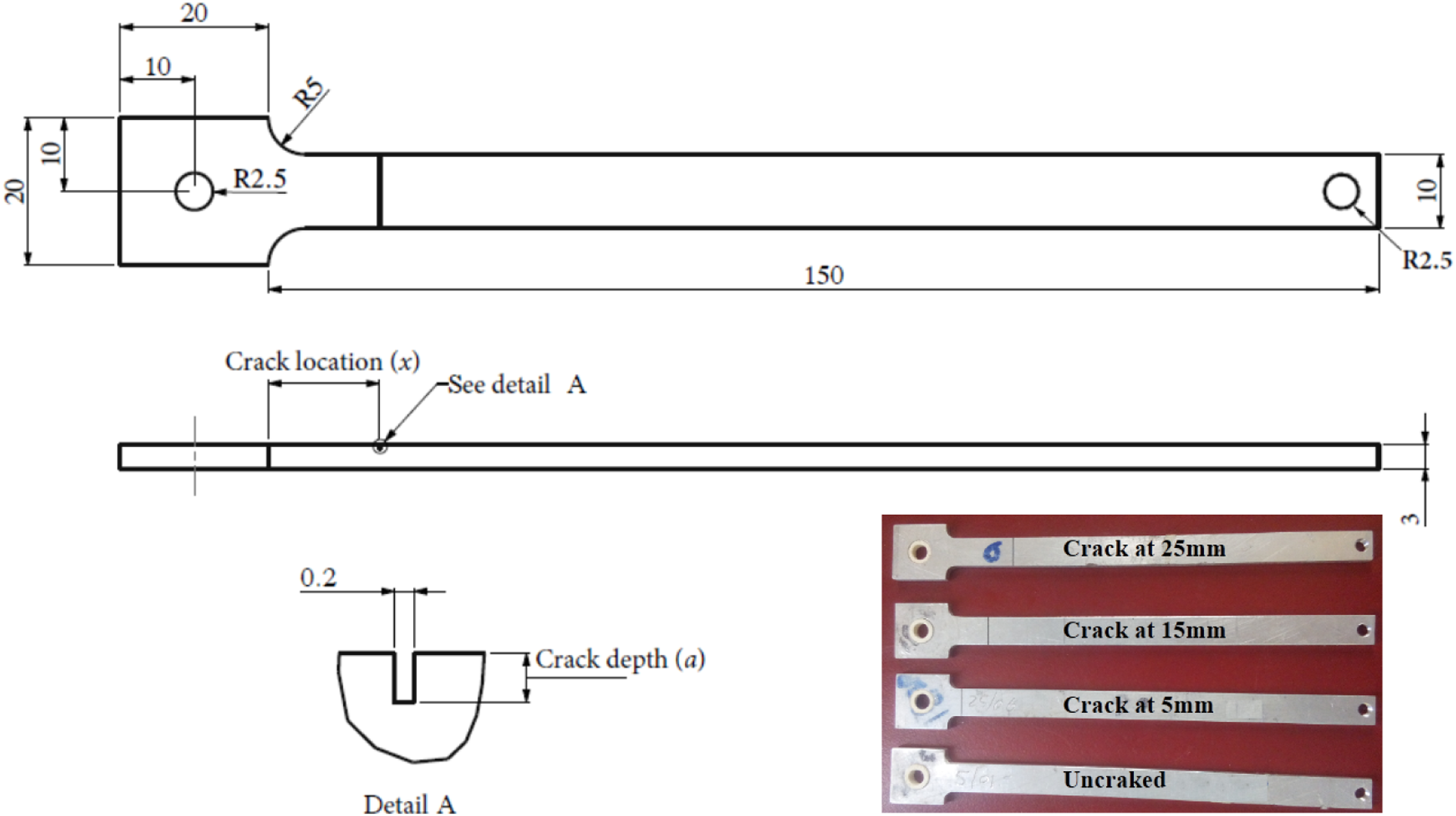

Each arrangement results in the induction of a fracture of a predetermined width which is 0.2 mm. Initial crack depth is given to be 0.5 mm, and it will grow with fracture propagation until it reaches a depth where it can cause catastrophic failure. To preserve the necessary dimensional precision, the specimens are produced using Computerized Numerical Control (CNC) wire cutting. To minimize experimental mistakes, each set of position and crack depth is represented by three separate samples.

Experimental setup

The specimen has 0.5 mm starting crack that naturally spreads under strain. Five distinct temperatures are evaluated on each configuration: room temperature, 50°C, 100°C, 150°C, and 200°C. The maximum temperature is selected to be significantly lower than half of Al-2024 melting point in order to prevent the potential of recrystallization.

As indicated in Figure 2, the entire experimental setup may be broken down into four components: vibrating setup, a heating setup, data gathering, last but not the least a propagation capture. A modal exciter (MS-100), a signal generating source (TENLEE 9200), and a power amplifier (MODAL LA-200) are utilized for the vibration setup. The specimen is subjected to a continuous displacement load of 5 mm thanks to MODAL LA-200 for producing a sine wave with a constant 5 V (peak to peak). Beam specimens with pre-selected fracture depths placed in same spotare installed on the modal exciter bearing fixed-free state. An accelerometer is fastened at specimen’s free end in order to gauge the dynamic response spread across a frequency spectrum. Entire system’s dynamic response driven predominantly by the movement of the specimen at it’s free end owing to resonance, can be calculated using any observable response because of the solid attachment between the exciter and the specimen.

Figure 2.

Experimental setup with schematic.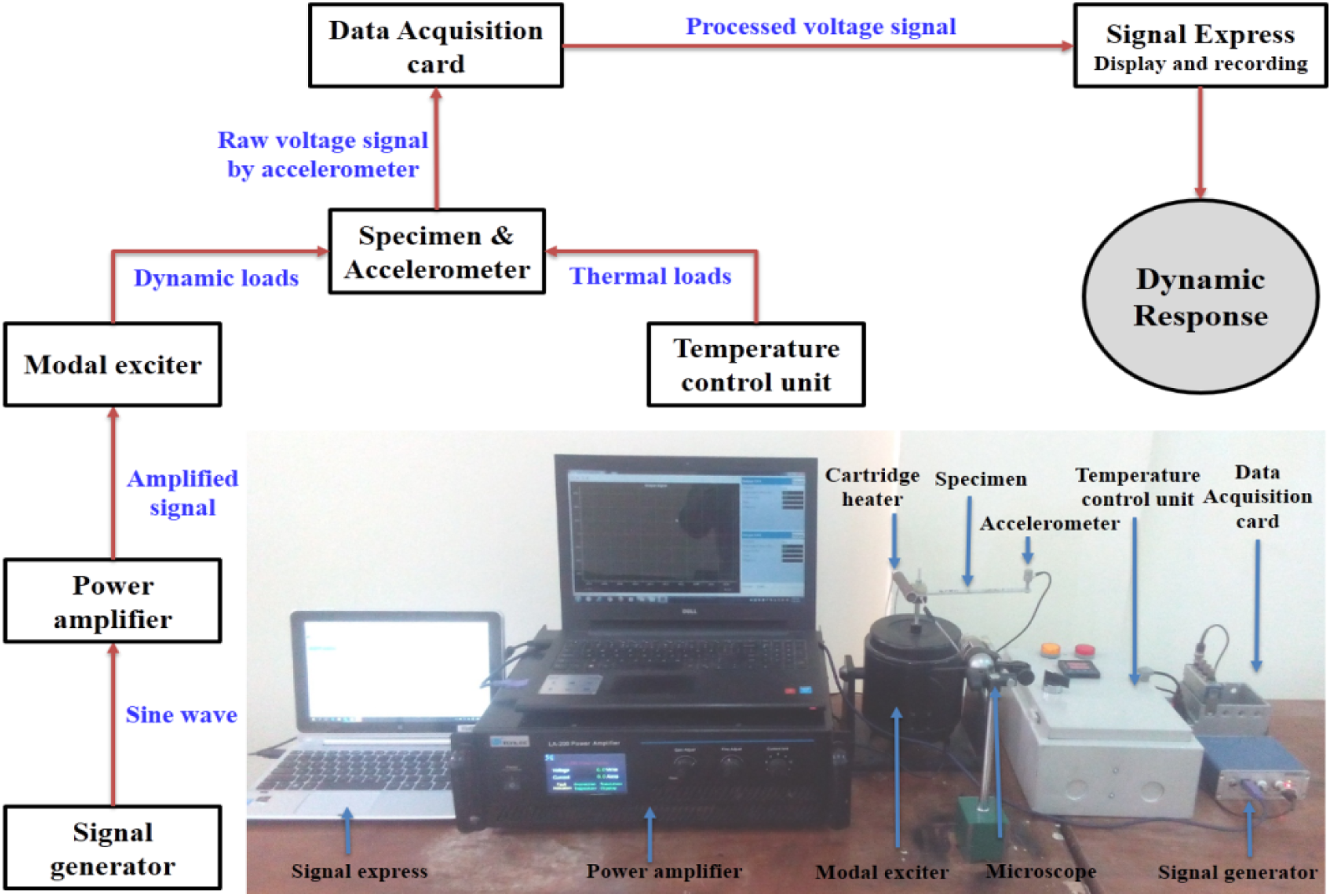

Using the power amplifier, the signal generator produces a sine wave of 5 V (peak to peak constant), which causes the specimen to experience a consistent 5 mm displacement loading. Beam specimens with pre-selected fracture depths placed in same spot are installed on a modal exciter bearing fixed-free state. At the specimen’s free end, an accelerometer is fastened in order to gauge the dynamic response spread across a frequency spectrum. Entire system’s dynamic response driven predominantly by the movement of the specimen at it’s free end owing to resonance, can be calculated using any observable response because of the solid attachment between the exciter and the specimen.

Measurements are collected based on time domain using National Instruments Signal Express and a DAQ (data acquisition) card NI-9174. In the Signal Express, under the analysis modules ‘Amplitude and Levels’ and ‘Power Spectrum’ are selected. In the first, the genuine response frequency amplitude is calculated while in the latter the real response frequency value is calculated. The frequency is steadily declining. The amplitude of vibration is similarly decreased in the frequency drop case. In order to obtain the shaker’s maximum amplitude, a new value lower frequency is chosen. Up until the subsequent frequency decrease, the specimen’s new fundamental frequency is maintained. Up to the specimen’s catastrophic breakdown, this process is repeated. When the specimen no longer shows amplitude at its free end, it has failed. A digital microscope (Dino-lite) with a magnification of 200x is used to determine the modal frequency and propagation fracture depth for each specimen. In Figure 3, a thorough experimental plan for fracture propagation is displayed.

Figure 3.

Experimental scheme elaboration.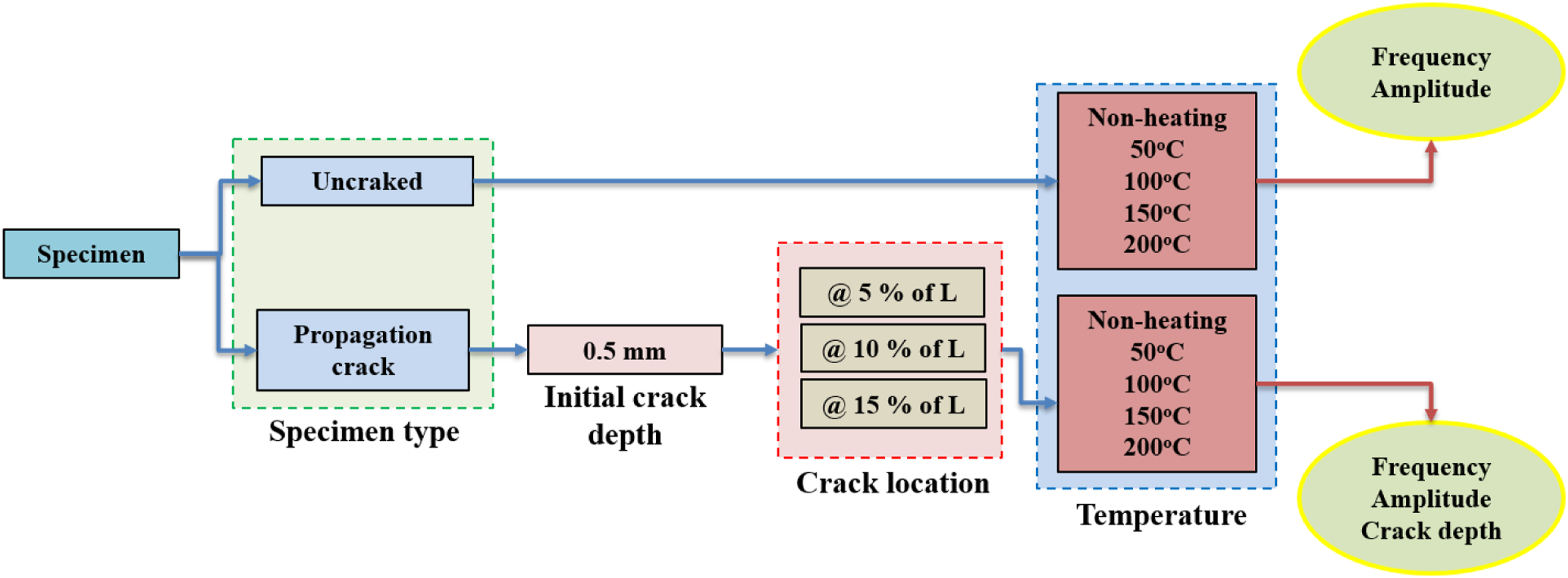

Methodology

Analytical formulation for thermo-mechanical loads

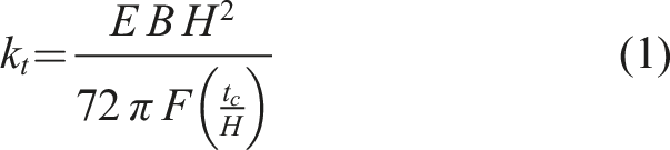
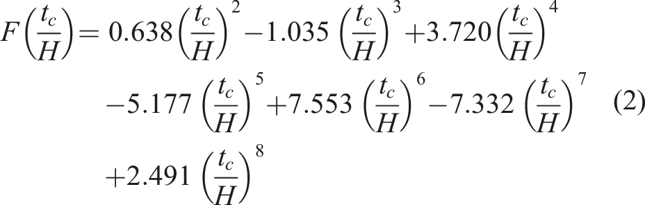
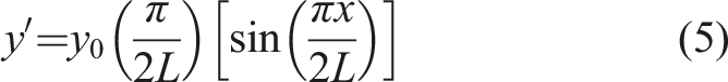
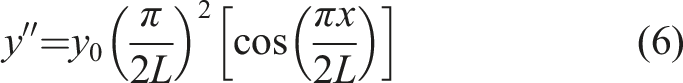
The influence of fracture depth is expressed analytically in this section as the decreased stiffness of a representative spring. As a result, such alteration in stiffness impacts on the structure’s general dynamic response to an external stress. Additionally, we introduced this formulation in our most recent works.^52,53 Figure 4 illustrates the modelling of the crack as a massless torsional spring using a cantilever beam. Ostachowicz et al.’s⁶ description of the torsional spring’s stiffness is illustrated in equation (1). The Rayleigh quotient is used to define the link between dynamic response and fracture depth in terms of natural frequency.

k_{t} = \frac{E B H^{2}}{72 π F (\frac{t_{c}}{H})}

(1)

F (\frac{t_{c}}{H}) = 0.638 {(\frac{t_{c}}{H})}^{2} - 1.035 {(\frac{t_{c}}{H})}^{3} + 3.720 {(\frac{t_{c}}{H})}^{4} - 5.177 {(\frac{t_{c}}{H})}^{5} + 7.553 {(\frac{t_{c}}{H})}^{6} - 7.332 {(\frac{t_{c}}{H})}^{7} + 2.491 {(\frac{t_{c}}{H})}^{8}

(2)

E I \frac{\partial^{4} y}{\partial x^{4}} + ρ A \frac{\partial^{2} y}{\partial t^{2}} = 0

(3)

y (x) = y_{0} [1 - \cos (\frac{π x}{2 L})]

(4)

y^{'} = y_{0} (\frac{π}{2 L}) [\sin (\frac{π x}{2 L})]

(5)

y^{″} = y_{0} {(\frac{π}{2 L})}^{2} [\cos (\frac{π x}{2 L})]

(6)

Where, H is height of the beam, width of the beam is given by B, E is modulus of elasticity, t_c shows crack depth, and

F (\frac{t_{c}}{H})

is a crack function. Free bending vibration of a beam is defined by a renowned differential equation, see equation (3). Applying the boundary conditions

y (0) = 0, {y^{'} |}_{@ x = 0} = 0

and

{y^{″} |}_{@ x = L} = 0

to determine the mode shapes as indicated by equations (4)–(6).

y_{0}

is the expected mode shape deflection and x is the crack location from the fixed end. According to equation (7), the bending moment can be calculated from the beam’s curvature and flexural stiffness (EI). The strain and the consequent strain energy due to bending can be used to compute the total strain energy, as illustrated in equations (8) and (9). Equations (10) and (12), published by Majid et al,⁵⁴ can be used to determine changes in strain energy and the natural frequency. They employed the Generalized Differential Quadrature (GDQ) technique to find the intrinsic natural frequency and mode shapes of the broken/cracked beam.

M = E I y^{″}

(7)

u = \frac{E I}{2} \int_{0}^{L} {(y^{″})}^{2} d x

(8)

u = \frac{E I}{64} π^{4} [\frac{1}{L^{3}}] {(y_{o})}^{2}

(9)

∆ u = \frac{M^{2}}{2 k_{t}}

(10)

∆ ω_{n c} = \frac{∆ u}{2 u} ω_{n}

(11)

ω_{n c} = ω_{n} - ∆ ω_{n c}

(12)

Figure 4.

Cantilever beam with a crack investigated as a mass less torsional spring.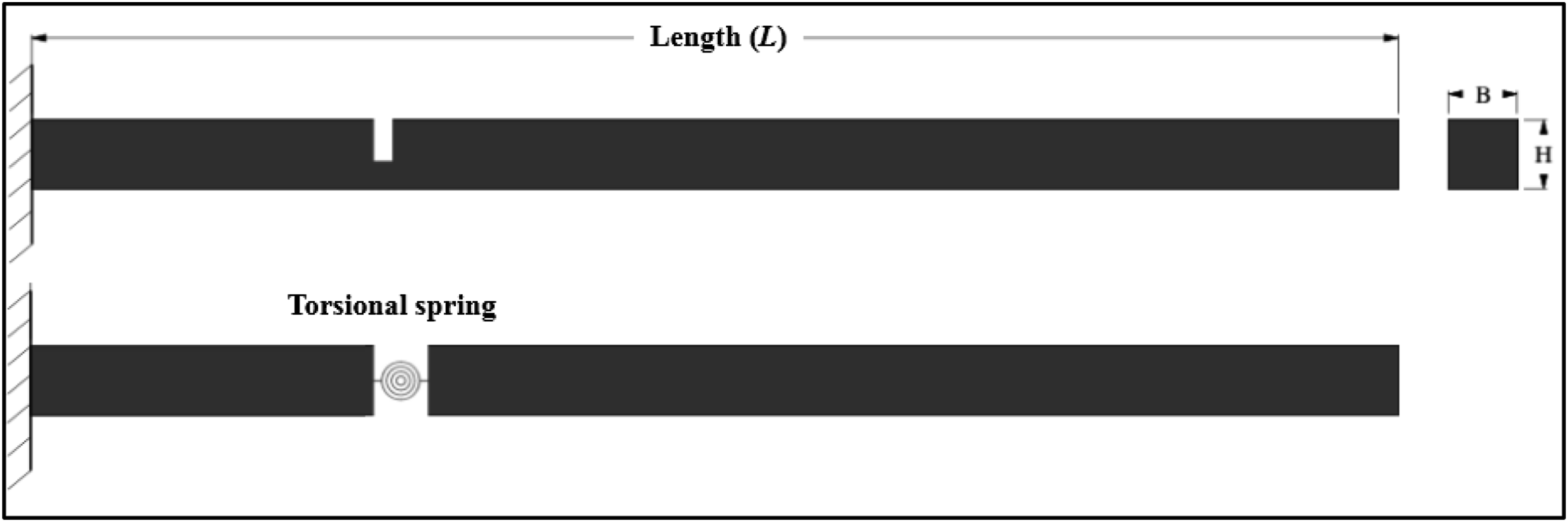

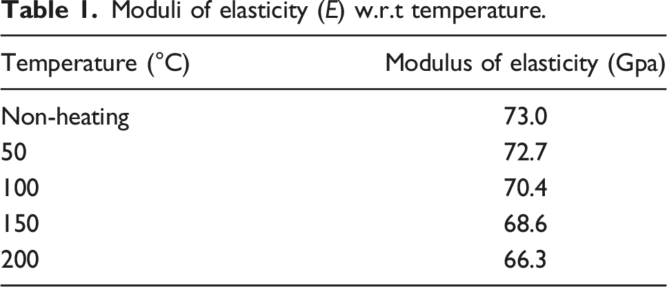
A generalized equation for $ω_{n c}$ can be created by combining equations (3) and (12), as seen in equation (13). All of the variables utilized in the analytical formulations are condensed in this equation. It may be deduced that the $ω_{n c}$ is independent of the mode shape and material parameters’ initial assumed values. The intrinsic frequency of an uncracked beam or at preceding the crack depth, the crack’s position, and the geometry of specimen, all play a role in this. As shown in Figure 5, an accelerometer is installed on the specimen’s end to assess the dynamic response at various fracture depths. Irvin⁵⁵ thus provides the natural frequency (undamped) of the beam with the end mass, as stated in equation (14).

ω_{n c} = {[1 - {\frac{72 π I F (\frac{t_{c}}{H})}{B H^{2} L} {(\cos 〈 \frac{π x}{2 L} 〉)}^{2}}] ω}_{n}

(13)

ω_{n m} = \sqrt{\frac{3 E I}{(0.2235 ρ_{L} L + m) L^{3}}}

(14)

ω_{n c} = [1 - {\frac{72 π I F (\frac{t_{c}}{H})}{B H^{2} L} {(\cos 〈 \frac{π x}{2 L} 〉)}^{2}}] \sqrt{\frac{3 E I}{(0.2235 ρ L + m) L^{3}}}

(15)

Where, u is the strain energy subsequently ∆u is the change in strain energy, M shows bending moment,

{∆ ω}_{n c}

is difference in the natural frequencies of the cracked and uncracked beam and

ω_{n c}

is the natural frequency of a cracked beam.

ω_{n m}

is natural frequency of beam with the end mass,

ρ_{L}

is the mass per unit length while

m

is the end mass (it’s basically the mass of accelerometer). To obtain equation (15), showing the temperature-dependent modulus of elasticity of the beam by E, apply equations (13) and (14) in combination. To determine the broken beam natural frequency at various temperatures, one can use the variation in E. The crack depth can be calculated using the dynamic response to thermomechanical stresses using this modal frequency. Table 1⁵⁶ displays the difference of the stiffness parameters with the variation of temperature from non-heating to 200°C.

Figure 5.

Schematic of a cantilever beam having end mass.

Table 1.

Moduli of elasticity (E) w.r.t temperature.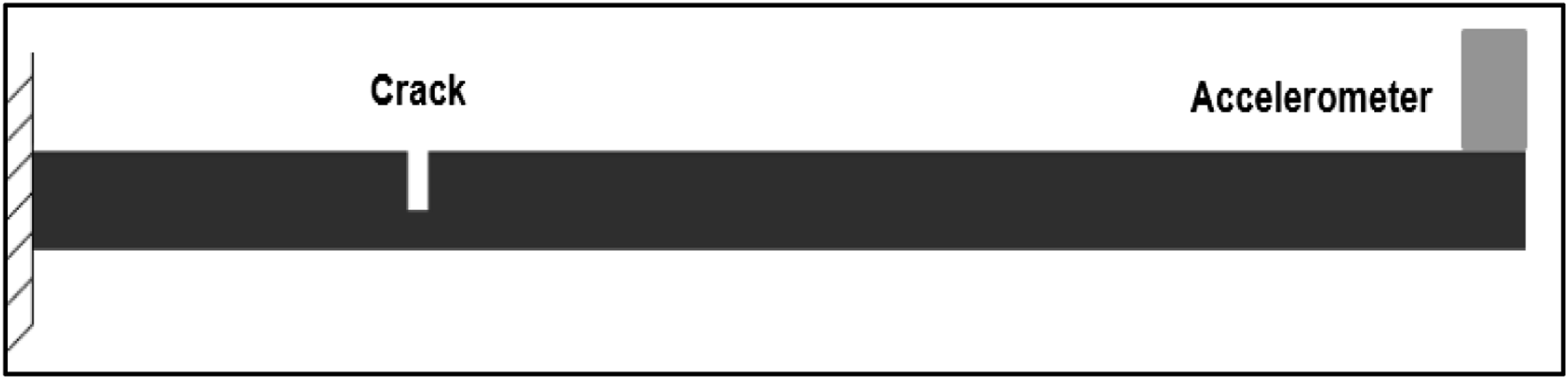

Temperature (°C)	Modulus of elasticity (Gpa)
Non-heating	73.0
50	72.7
100	70.4
150	68.6
200	66.3

Application of neural network

In contrast to the empirical relation ANN is used to establish a trend to predict the damage quantification of metallic beams for the parameters discussed below. ANN delivers swift adaptability while preserving the generalization of the trend with accurate and appropriate application for numerous problems. Owing to these attributes ANNs are widely being used and has a great potential for estimating damage severity along with location in structures⁵¹

The input layer consist of three parameters namely temperature, frequency and amplitude. Feed forward neural network is used with back propagation algorithm. There is a single hidden layer consisting of 13 neurons that connects with a two output parameter i.e. crack depth and crack location. Each parameter is linked with hidden neuron with input weightage factor i.e. Wx,i. Where x denote the neuron and i denote the parameter. The hidden neuron is connected with output parameter with output weightage factor i.e. W. Each neuron in hidden and output layer has bias value denoted by b and B respectively. Figure below shows the diagram of the neural network. (Figure 6).

Figure 6.

Network diagram.

This network is conventionally used to estimate the weights and bias value of each neuron. In back propagation of neural network, gradient decent algorithm is used to minimize the error function. The network is trained by supervised learning i.e. input data is organized prior to training of neural network. The error function move back and forth updating the input and output weights with bias value to achieve the desired output. The training process start by first initializing the weights and biasness at random values. These random weights and biasness are then fed into network to update the model. The input layer is connected with each neuron of hidden layer with some weightage factor that changes after number of iterations. The information is transferred between input and hidden layer by means of activation function. Each hidden neuron is connected with output parameter by weightage factor that updates during back propagation. The error function is computed based on difference between the target value and trained value. The next step is to calculate the correction factor for output weight and bias value. The error function of hidden neuron is then calculated by summing the product of input weight and error function of output layer and then multiplying it with derivative of activation function. The subsequent delta of input weights and bias value of each neuron is then calculated. The final step is to update the input and output weights with their bias values. The process is based on back propagation that continuously calculates error function and update the model until the stopping criteria is achieved. MATLAB ® toolbox is used for the building and training of ANN. ANN is trained over the same range of experimental data as used to derive the empirical equation. This establishes a robust basis for trend development. Primarily, the network is trained by three input variables namely Temperature, Frequency and Amplitude against the two output variables as Crack depth and Crack location. A range of data is selected for this purpose and a set of size 75 is selected to train the network. The overall size of training array is 75 rows and 5 columns.

Results and discussion

Experimental results

There are four variants available: Uncracked, Cracked at a length of 5%, 10% and 15% of L. A brand-new specimen with a crack depth of 0.5 mm is placed/mounted on the shaker at varioustemperatures at the beginning of each experiment. Measurements are made while the specimen operates at its native frequency. The reduction in amplitude is seen as a sign that the specimen’s inherent frequency has changed. A wooden mallet is used for the impact test once more in order to determine the new modal frequency. Up to the specimen’s catastrophic breakdown, this process is repeated. Figure 7 displays the image taken simultaneously while measuring the crack depth using a microscope. Figure 8 plots natural frequencies and their corresponding dips in relation to the fracture depth ratio.

Figure 7.

The evolution of crack propagation in the samples.

Figure 8.

Natural frequency V/S crack depth for a propagating cracklocated at 5% of total length.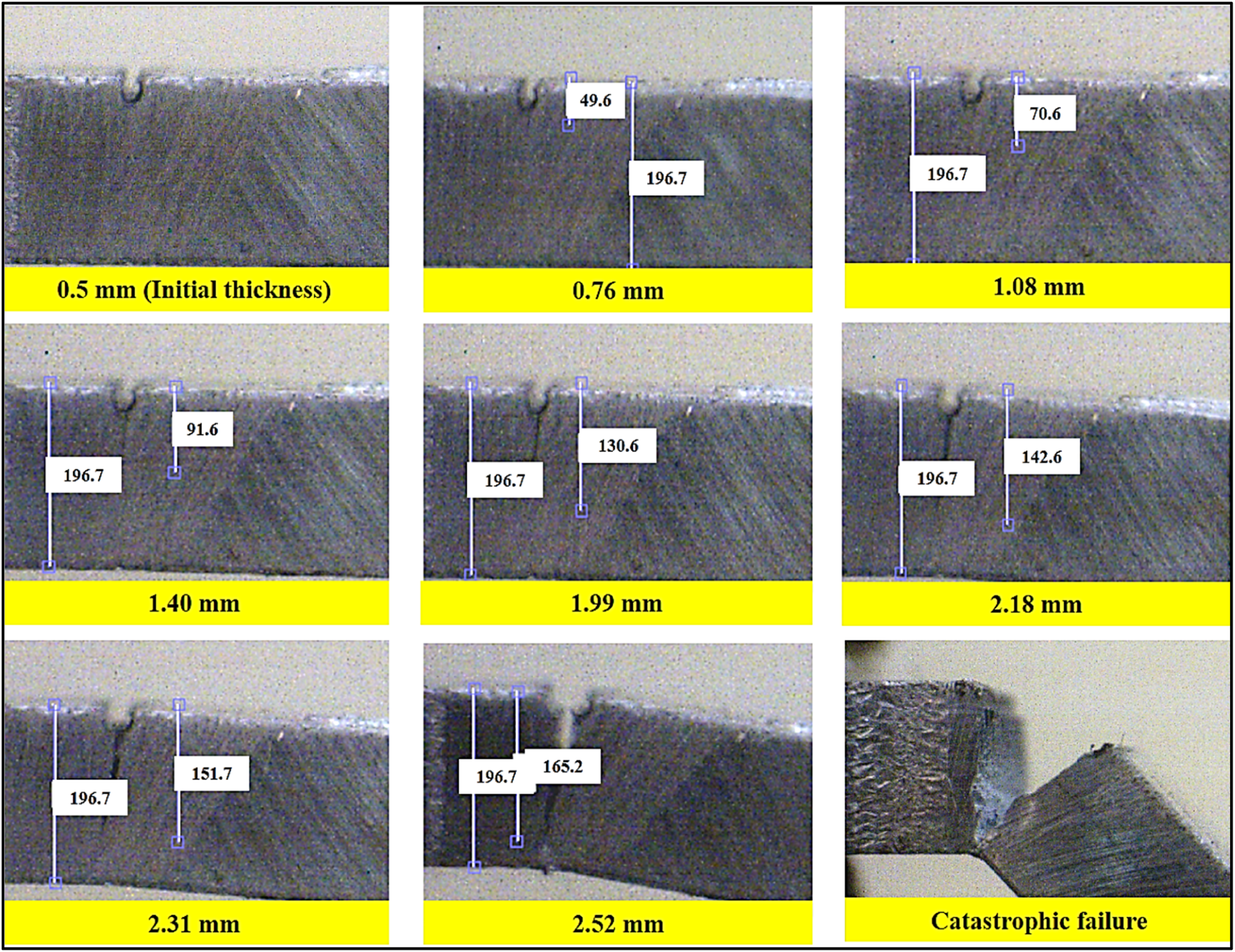

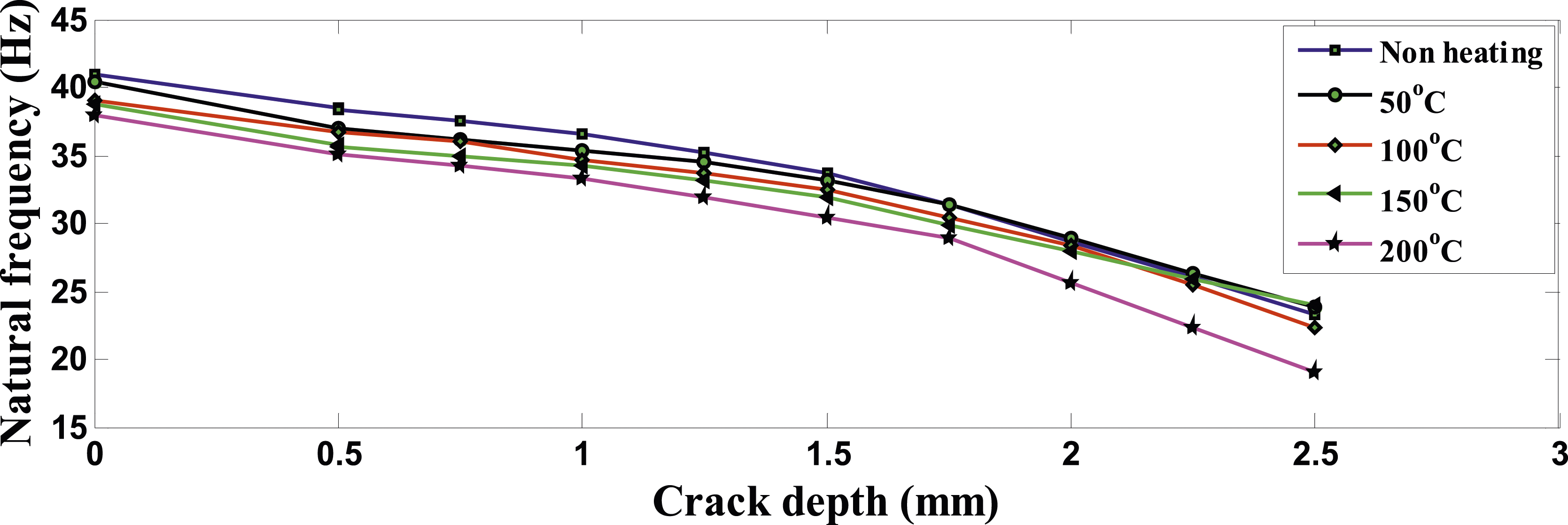
The specimen’s natural frequency value at a 0.5 mm fracture depth is its natural frequency. The fracture will initiate wideningas soon as the load is introduced, and the specimen vibrates at its natural frequency. As seen by the graphs, this propagation will lessen stiffness, which will ultimately result in a fall in natural frequency. Up to its catastrophic failure, the lowest value is reached. The variation in amplitude response w. r.t a propagating crack is also evaluated in light of initial crack depth, as depicted in Figure 9 for a crack that is 5% of the total length at a certain temperature range. The decrease in stiffness due crack propagation results in increased responsesagainst the same magnitude of force. The results of amplitude and natural frequency are like first seeded crack. The fracture that is 15% of the total length long and has the highest natural frequency value and the lowest value of amplitude at the same magnitude of damage.

Figure 9.

Amplitude V/S crack depth for propagating crack located at 5% of total length.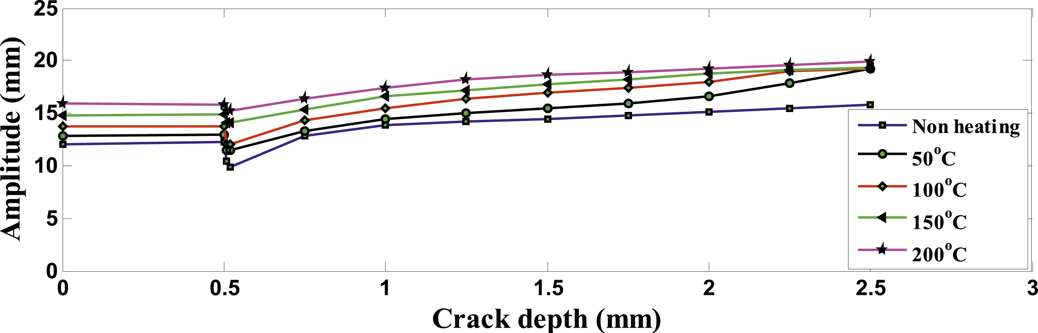

A notable observation made during crack propagation is that at a crack depth of around 0.5 mm, the natural frequency did not significantly vary in response to subsurface cracking. As a result, it was very challenging to determine the exact moment that subsurface cracking began. The first seeded crack depicted in Figure 8 does not appear to have changed under the microscope. On the other side, a dip in amplitude at 0.5 mm signifies the start of subsurface crack propagation, which can later help with preventative maintenance planning, as illustrated in Figure 9. Therefore, under thermomechanical stresses that accelerate fracture propagation by lowering structural stiffness, the amplitude response is given more weight.

The frequency and amplitude response is presented for temperature ranges ranging from non-heating to 200°C in order to visualize the impact of temperature change. For the same amount of damage, a structure’s natural frequency is decreased as temperature rises. On the other hand, amplitude rises as structural damping is decreased. This demonstrates how the temperature might affect thermomechanical loads’ failure rate.

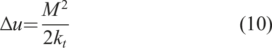
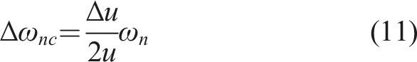
5%, 10%, and 15% of the total length of the crack are located for temperatures between zero and 200°C. For all temperature values, the value of natural frequency is larger for cracks that are at 15% of the total length, indicating that the stiffness of specimen is immune to crack locations that are distant from the fixed support. The subject structure becomes more elastic because of a crack that is near the fixed support, which results in a lower structural damping value. The structure with a lower value of natural frequency, thus, presents a larger value of amplitude response undergoing the same stress. It demonstrates that the placement of the crack has no bearing on the material damping. However, the placement of the crack may alter the structural damping. The underdamped response of the system to the damping and reduction in natural frequency, which is demonstrated in equation (16),⁵⁷ further supports this.

{x = X e}^{- ξ ω_{n} τ}

(16)

where,

x

represents the instantaneous amplitude,

ξ

gives the damping and

τ

is the time.

Empirical correlations

The proposed approach, which includes an empirical connection between the fracture depth, natural frequency, temperature, crack location and beam amplitude, can identify both the location and depth of the crack. For an empirical relationship to be formed, a sizable number of experiments are needed. Using the decline in natural frequency, temperature and amplitude difference, this empirical relation is anticipated to be able to forecast the fracture depth. To determine the percentage reliability of the outcomes in light ofthe experimental data as described through equation (17),⁵⁸ the percentage replication (PR) criterion is frequently utilized.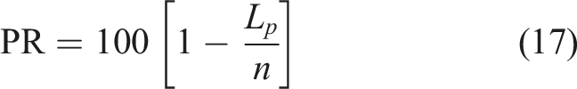

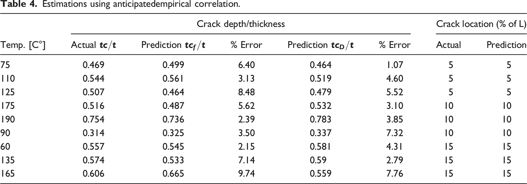
PR = 100 [1 - \frac{L_{p}}{n}]

(17)

Here,

L_{p}

is the number of changing parameters and

n

is the total number of experiments. Five temperatures and a total of three places are taken into account in this work. Three samples are evaluated in each location and temperature combination. This will increase the data set’s dependability to 82%, indicating that the results predicted using these empirical correlations will be 82% accurate.

The reaction and temperature are taken into account when developing the suggested methodology. Interpolation is used to identify three permutations of fracture depth and position for amplitude difference and frequency drop separately using the data that is currently available. Because the same amplitude difference and frequency drop may be attained using three distinct sets of fracture depth and location, these three combinations are practical. The distinctive feature between each set of crack depths at a certain site determined by amplitude difference and frequency drop is then measured. The most precise location and crack depth will be indicated by the anticipated values with the smallest difference based on amplitude difference and frequency drop. Figure 10 displays a thorough diagram for determining the depth and position of cracks.

Figure 10.

Plan for predicting crack location and depth.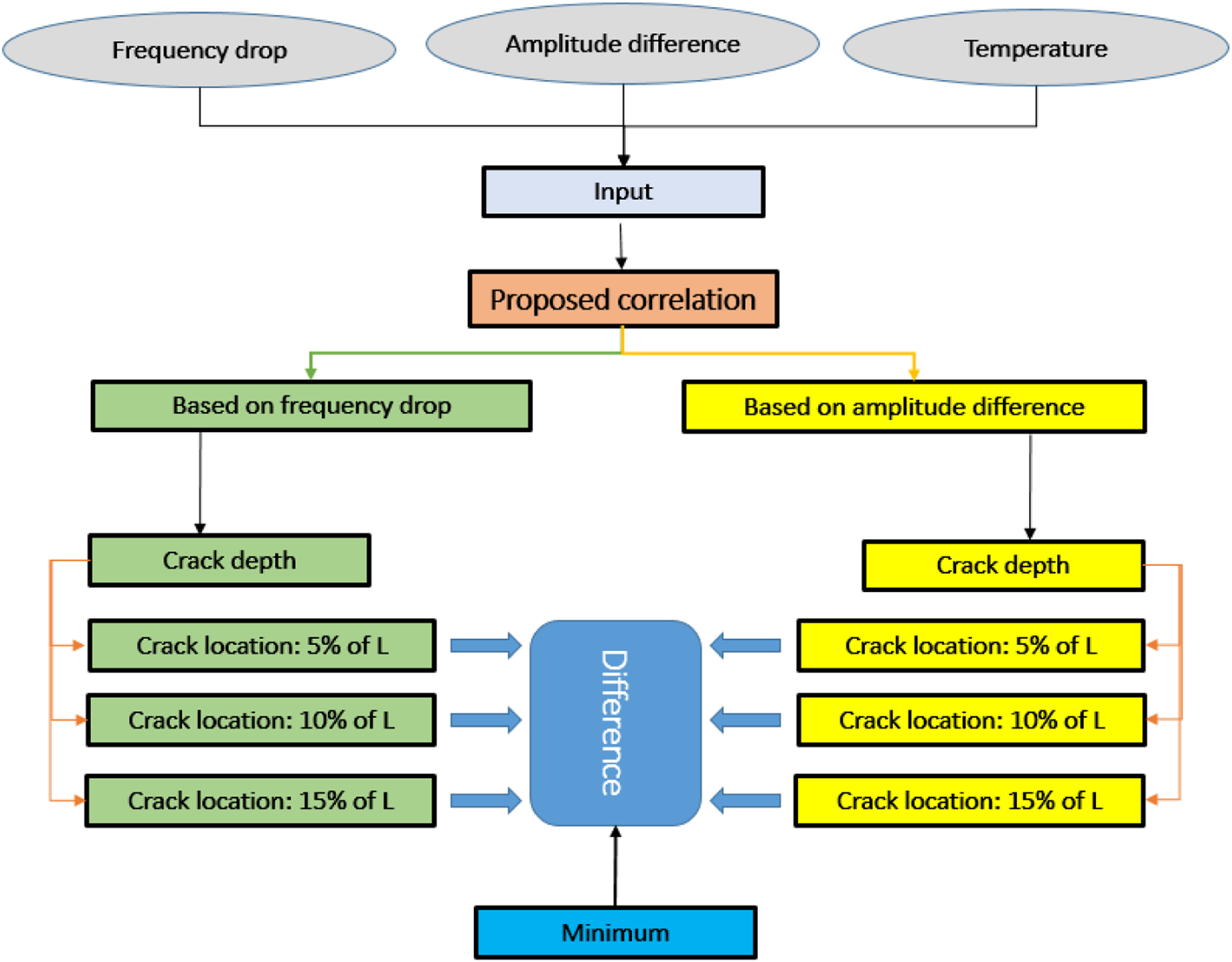

Three locations will have six universal correlations owing to certain response parameters. Six global correlations are derived from these correlations, and three are used to calculate the crack depths by amplitude difference and three by natural frequency difference. One location is represented by one set of values for the crack depth. Therefore, the variation in these crack depths is due to one site, and this location will be used to determine where the actual crack will be. The real location of the crack will be at the point where the difference in crack depth is least. You can use these empirical correlations to determine how a fracture spreads from its inception until its failure. A fair agreement is found between the values for the visually observed crack depth and the values determined from equation (15).

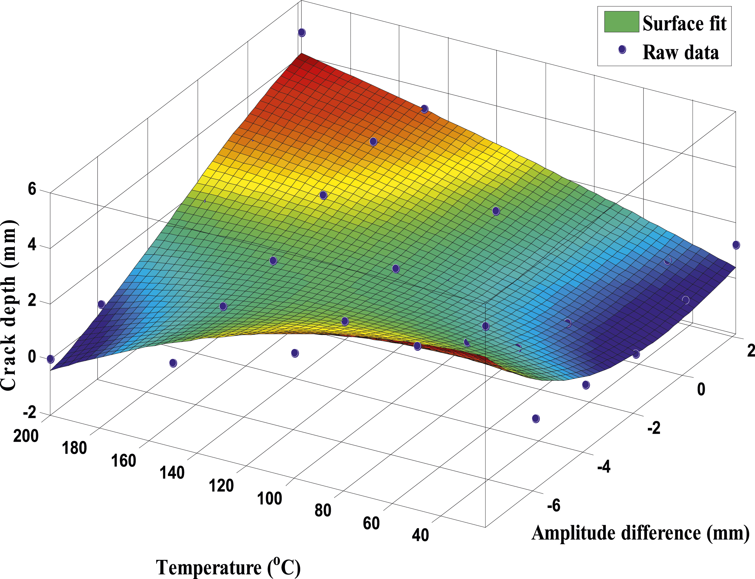
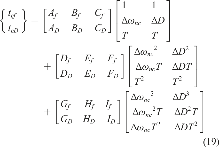
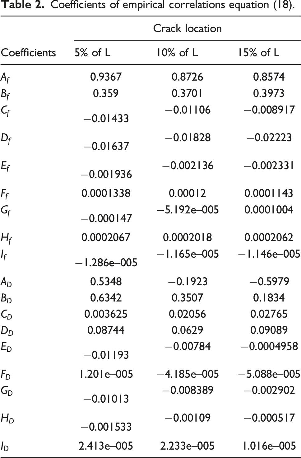
On the basis of the provided data, a curve fitting is done to produce a universal empirical correlation that can account for a variety of frequency and sample lengths, as indicated in equations (18) and (19). The formulation of equation (19) takes into account temperature, amplitude differential, and frequency drop. As a result, the first matrix represents the polynomial coefficient, and the second is dependent on the relevant temperature and dynamic response parameter values. Figures 11 and 12 exhibit the crack depth in correlation with temperature or as a its function, drop in frequency, and amplitude difference. The majority of the data points are compatible with this polynomial curve fit. Although a small fraction of the population is still uninsured, the forecast percentage will be definitely close.

Figure 11.

Depiction of surface fit and experimental data for empirical correlation in light of frequency drop for crack located at 5% of L.

Figure 12.

Surface fit and experimental data for empirical equationencompassing amplitude difference for a crack located at 5% of L.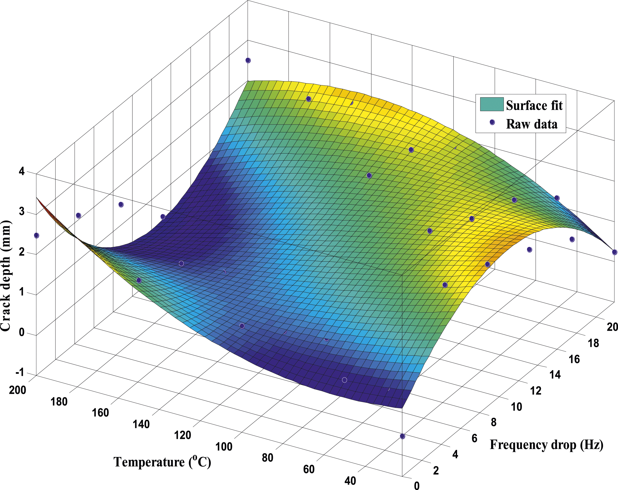

Experimental results are shown here along with the results obtained from a global empirical correlation. Both these results show a profound agreement. The Within a 10% error, a worldwide empirical relationship can predict about 82% of the valid dates. The existence of a fracture can alter the specimen’s material characteristics, resulting in a reduction in its natural frequency while introducing amplitude fluctuation ultimately leading to catastrophic collapse. If the dip in frequency, temperature and amplitude fluctuations are known, mathematically, then empirical correlations may be found from these patterns that can then be utilized to find the location of fracture and its depth. For evaluating damage to metallic structures in situ, this equation can be quite helpful. In situ damage assessment can be done extremely well using these empirical relationships. Higher frequency drops and amplitude differences have great damage prediction accuracy.

t_{c} = f ({∆ ω}_{n c}, ∆ D, T)

(18)

{\begin{cases} t_{c f} \\ t_{c D} \end{cases}} = [\begin{array}{l} A_{f} & B_{f} & C_{f} \\ A_{D} & B_{D} & C_{D} \end{array}] [\begin{array}{l} 1 & 1 \\ {∆ ω}_{n c} & ∆ D \\ T & T \end{array}] + [\begin{array}{l} D_{f} & E_{f} & F_{f} \\ D_{D} & E_{D} & F_{D} \end{array}] [\begin{array}{l} {∆ ω}_{n c}^{2} & {∆ D}^{2} \\ {∆ ω}_{n c} T & ∆ D T \\ T^{2} & T^{2} \end{array}] + [\begin{array}{l} G_{f} & H_{f} & I_{f} \\ G_{D} & H_{D} & I_{D} \end{array}] [\begin{array}{l} {∆ ω}_{n c}^{3} & {∆ D}^{3} \\ {∆ ω}_{n c}^{2} T & {∆ D}^{2} T \\ {{∆ ω}_{n c} T}^{2} & {∆ D T}^{2} \end{array}]

(19)

where,

t_{c D}

is the crack depth prediction in light of amplitude difference,

t_{c f}

is crack depth estimation based on drop in natural frequency,

∆ D

is the amplitude difference,

{∆ ω}_{n c}

is natural frequency drop,

T

is selected temperature,

A_{f}, B_{f}, C_{f}, D_{f}, E_{f}, G_{f}, H_{f}, I_{f}

are the coefficients of empirical correlation that are based on frequency drop and the temperature data for a crack located at 5% of L,

A_{D}, B_{D}, C_{D}, D_{D}, E_{D}, G_{D}, H_{D}, I_{D}

are the coefficients of empirical associationas expressed in Table 2.

Table 2.

Coefficients of empirical correlations equation (18).

Coefficients	Crack location
Coefficients	5% of L	10% of L	15% of L
$A_{f}$	0.9367	0.8726	0.8574
$B_{f}$	0.359	0.3701	0.3973
$C_{f}$	−0.01433	−0.01106	−0.008917
$D_{f}$	−0.01637	−0.01828	−0.02223
$E_{f}$	−0.001936	−0.002136	−0.002331
$F_{f}$	0.0001338	0.00012	0.0001143
$G_{f}$	−0.000147	−5.192e–005	0.0001004
$H_{f}$	0.0002067	0.0002018	0.0002062
$I_{f}$	−1.286e–005	−1.165e–005	−1.146e–005
$A_{D}$	0.5348	−0.1923	−0.5979
$B_{D}$	0.6342	0.3507	0.1834
$C_{D}$	0.003625	0.02056	0.02765
$D_{D}$	0.08744	0.0629	0.09089
$E_{D}$	−0.01193	−0.00784	−0.0004958
$F_{D}$	1.201e–005	−4.185e–005	−5.088e–005
$G_{D}$	−0.01013	−0.008389	−0.002902
$H_{D}$	−0.001533	−0.00109	−0.000517
$I_{D}$	2.413e–005	2.233e–005	1.016e–005

Validation of correlations and comparison with neural network

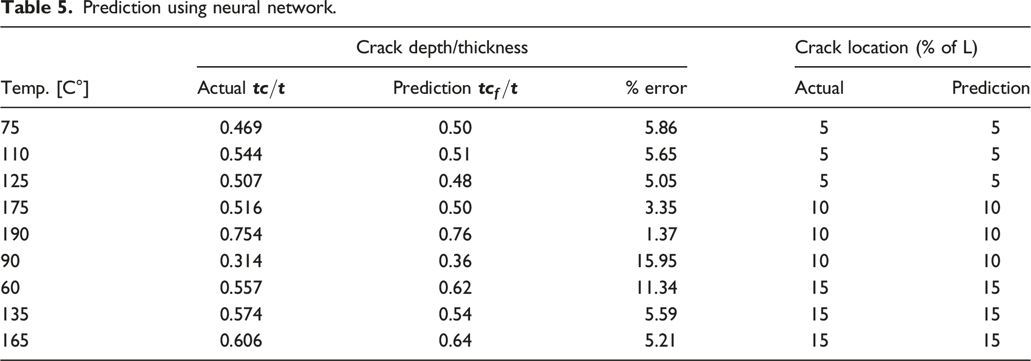
The network is trained using a supervised learning technique by sorting all of the trial data to reduce noise; this process improves network fitting while preserving trend generalization. Figure 13 illustrates the results of training using the Bayesian regularization technique, which yield an overall regression value of 0.98.

Figure 13.

Regeneration plot.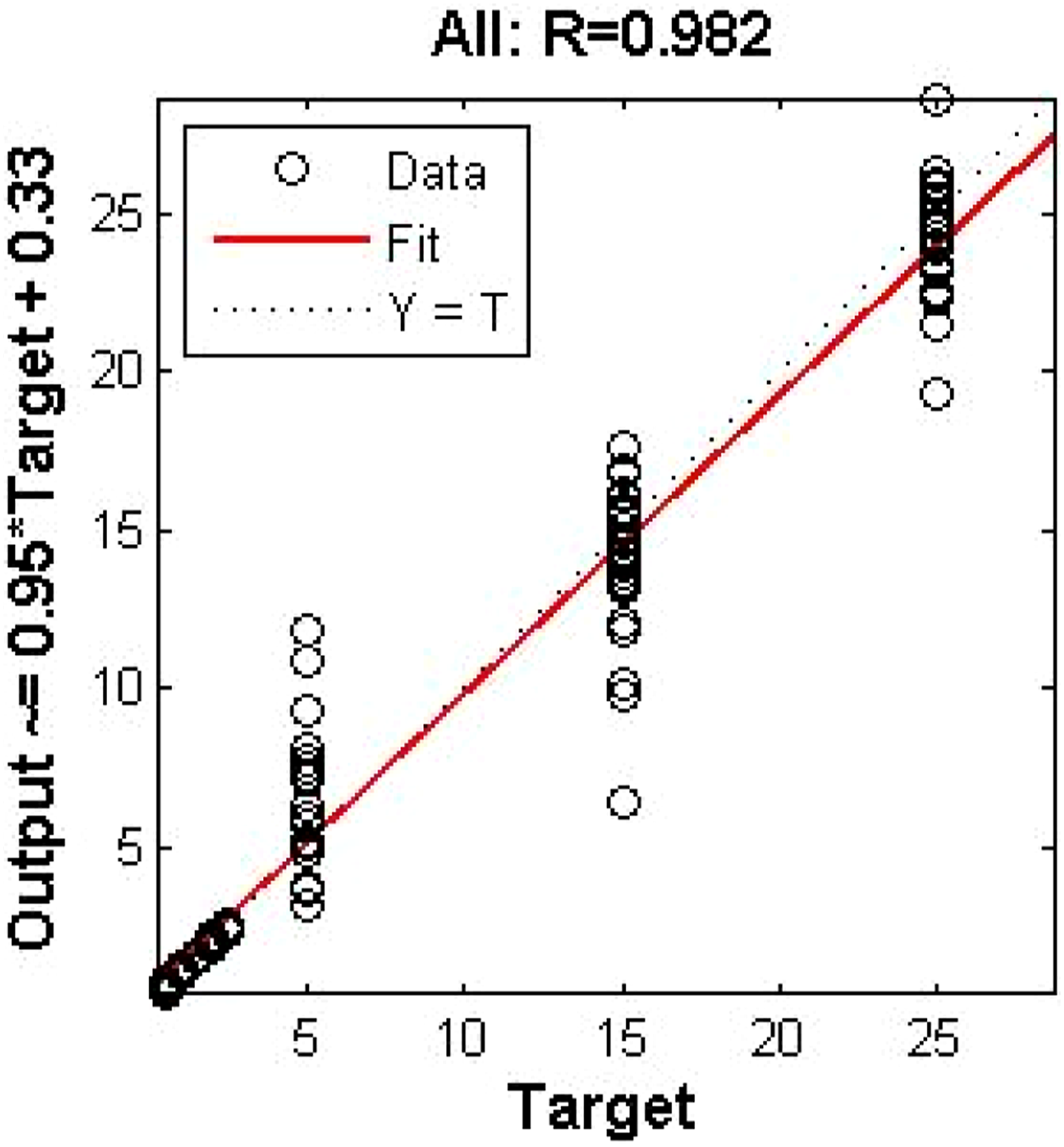

The training error achieved is significantly small and it is achieved in over 215 iterations as shown in Figure 14. In order to obtain the best possible regression and minimal error several trainings of the network are performed and while it varies every time, the values differ only slightly. The results obtained for the arbitrary data set are within the target of 10% error, indicating that the network has been successfully trained. Finding the depth and position of damage cracks is made possible by the promising outcomes. However, in some circumstances, experimenting with various neural network designs and parameter values can provide the best prediction.

Figure 14.

Training error plot.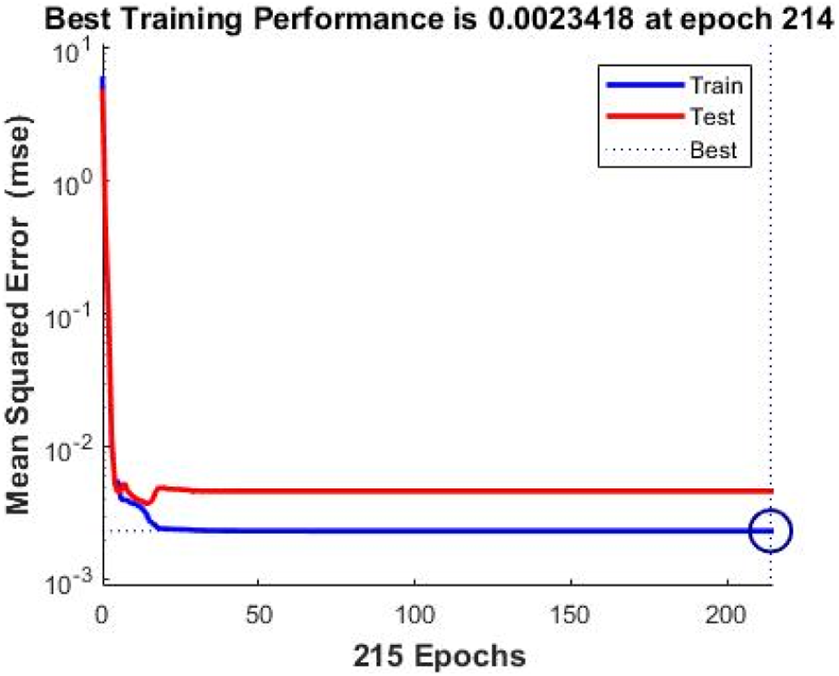

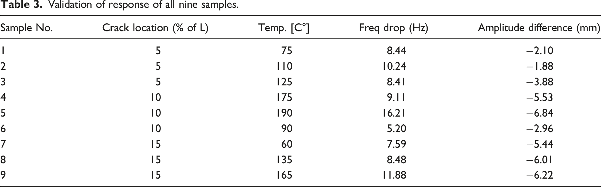
A total of nine samples were tested for damage assessment under various input parameters to broadly validate the empirical correlations shown in equation (19) and the neural network’s response. Three of the nine options are taken into account for each location for various response levels and temperatures. As illustrated in Table 3, the corresponding amplitude difference and frequency drop are calculated. As seen in Table 4, The results of the suggested correlation’s prediction are very comparable to those of reality. Using a neural network, the same results are reevaluated, and it is discovered that the results are even better with less error. Figure 15 displays images for experimental validation. The formula in equation (20) can be used to compute the crack depth to thickness ratio.

t c / t = F 1 / F 2

(20)

where, using MATLAB’s lmtool, F1 represents the image’s crack measurement while F2 represents its thickness measurement.

t

is sample thickness and

t c

is the crack depth.

Table 3.

Validation of response of all nine samples.

Sample No.	Crack location (% of L)	Temp. [C°]	Freq drop (Hz)	Amplitude difference (mm)
1	5	75	8.44	−2.10
2	5	110	10.24	−1.88
3	5	125	8.41	−3.88
4	10	175	9.11	−5.53
5	10	190	16.21	−6.84
6	10	90	5.20	−2.96
7	15	60	7.59	−5.44
8	15	135	8.48	−6.01
9	15	165	11.88	−6.22

Table 4.

Estimations using anticipatedempirical correlation.

Temp. [C°]	Crack depth/thickness					Crack location (% of L)
Temp. [C°]	Actual $t c / t$	Prediction ${t c}_{f} / t$	% Error	Prediction ${t c}_{D} / t$	% Error	Actual	Prediction
75	0.469	0.499	6.40	0.464	1.07	5	5
110	0.544	0.561	3.13	0.519	4.60	5	5
125	0.507	0.464	8.48	0.479	5.52	5	5
175	0.516	0.487	5.62	0.532	3.10	10	10
190	0.754	0.736	2.39	0.783	3.85	10	10
90	0.314	0.325	3.50	0.337	7.32	10	10
60	0.557	0.545	2.15	0.581	4.31	15	15
135	0.574	0.533	7.14	0.59	2.79	15	15
165	0.606	0.665	9.74	0.559	7.76	15	15

Figure 15.

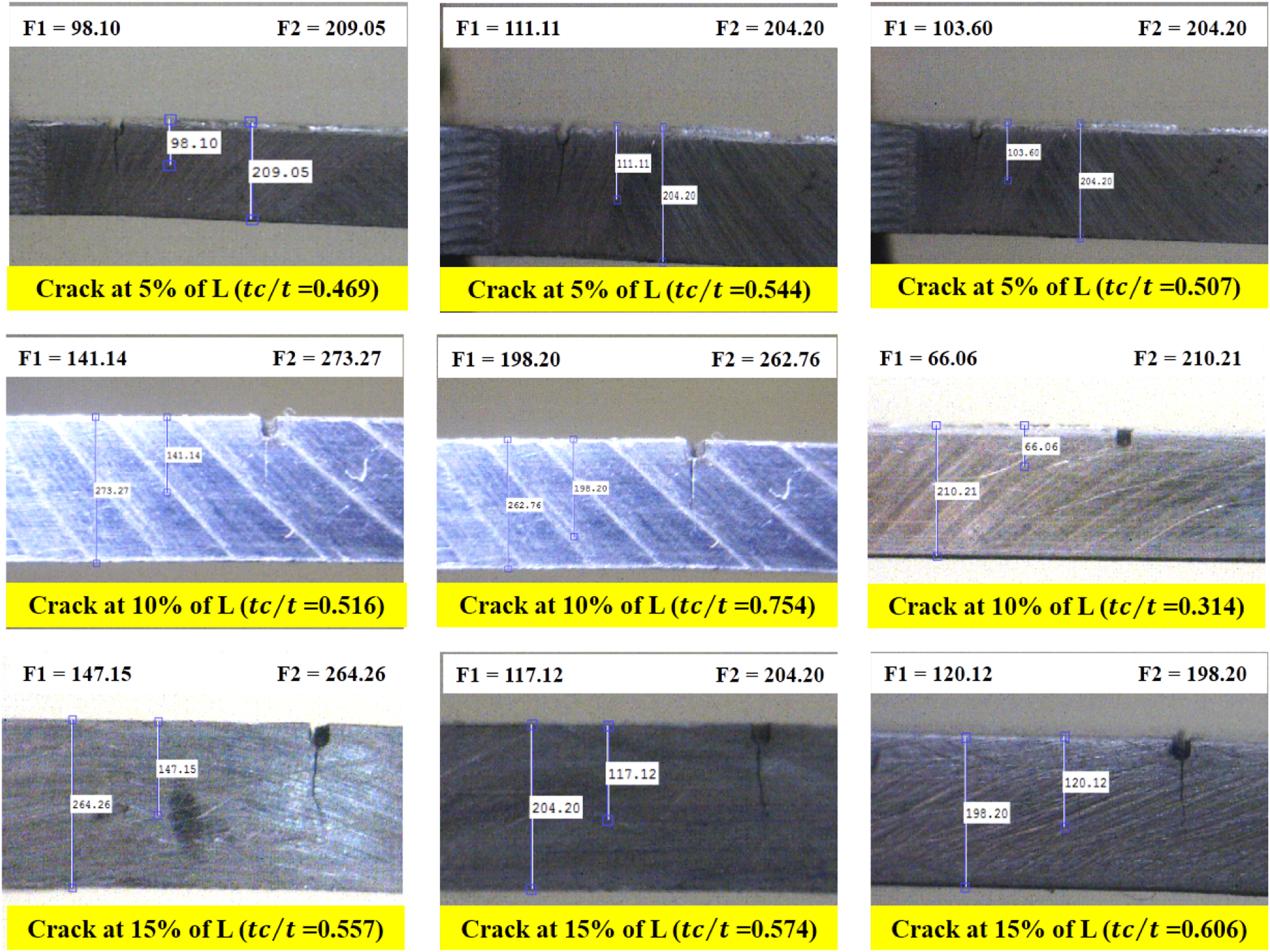
Specimen images for experimental validation.

The same experimental data from the initial samples is used to carry out the damage prediction methods for both novel empirical methodologies and neural networks. The outcomes demonstrate how effective the unique empirical technique is at more accurately predicting the outcomes. The findings from the neural network are comparable, although some random samples show larger amounts of error (>10%), which may be a result of network training’s limitations.(Table 5).

Table 5.

Prediction using neural network.

Temp. [C°]	Crack depth/thickness			Crack location (% of L)
Temp. [C°]	Actual $t c / t$	Prediction ${t c}_{f} / t$	% error	Actual	Prediction
75	0.469	0.50	5.86	5	5
110	0.544	0.51	5.65	5	5
125	0.507	0.48	5.05	5	5
175	0.516	0.50	3.35	10	10
190	0.754	0.76	1.37	10	10
90	0.314	0.36	15.95	10	10
60	0.557	0.62	11.34	15	15
135	0.574	0.54	5.59	15	15
165	0.606	0.64	5.21	15	15

Conclusion

A novel methodology is proposed to predict the crack depth in an Aluminum 2024 cantilever beam, operating at a modal frequency by its dynamic response values including frequency drop and amplitude difference. Due to changes in stiffness, the dynamic response including frequency drop and amplitude also changes; this effect has also been investigated by varying temperature based on in situ working conditions. Experimental information for deepening cracks in various places is acquired. Based on the comprehensive results, a trend is obtained to establish relationships among crack depth, location and temperature for the first time for a cantilever beam operating under thermo-mechanical loads. Higher temperature reduces stiffness, which in turn reduces the frequency and causes a beam to vibrate more violently under the same load. Similar behavior is seen for cracks that are farther from the fixed support. Notable results are obtained for amplitude response in which the subsurface cracking is evident without showing any increase in crack propagating; this will be extremely beneficial for preventive maintenance and give warning well before catastrophic failure. To forecast the location and depth of cracks, a thorough schematic is developed and then compared with a neural network approach. In order to create thisreliable tool, empirical relations in light of global curve fit are developed using temperature and dynamic response. This tool is validated for both readily available data and arbitrary sample data. The projected outcomes are in line with the outcomes attained using the neural network and are well within the prediction range of 10%. Without interrupting the structural element’s normal processes, this approach can further be utilized to analyze the rate of crack propagation and its course.

Footnotes

Declaration of conflicting interests

The author(s) declared no potential conflicts of interest with respect to the research, authorship, and/or publication of this article.

Funding

The author(s) received no financial support for the research, authorship, and/or publication of this article.

ORCID iDs

Behzad Ahmed Zai

Najam us Saqib

References

Doebling

Farrar

Prime

. A summary review of vibration-based damage identification methods. Shock Vib 1998; 30: 91–105.

Fan

Qiao

. Vibration-based damage identification methods a review and comparative study. Struct Health Monit 2011; 10: 83–111.

Das

Saha

K Patro

. Vibration-based damage detection techniques used for health monitoring of structures a review. J Civ Struct Health Monit 2016; 6: 477–507.

Khorshidi

Soltani

. Diagnosis of type, location and size of cracks by using generalized differential quadrature and Rayleigh quotient methods. J Theor Appl Mech 2013; 43: 61–70.

Loya

Rubio

Fernandez-Saez

. Natural frequencies for bending vibrations of Timoshenko cracked beams. Contin Mech Struct Anal 2006; 290: 1–14.

Ostachowicz

Krawczuk

. Analysis of the effect of cracks on the natural frequencies of a cantilever beam. J Sound Vib 1991; 150: 191–201.

Batihan

. Vibration analysis of cracked beams on elastic foundation using Timoshenko beam theory. MS thesis. Ankara: Middle East Technical University, 2011.

Cannizzaro

De Los Rios

Caddemi

, et al. On the use of a roving body with rotary inertia to locate cracks in beams. J Sound Vib 2018; 425: 275–300.

Caddemi

Caliò

. Exact reconstruction of multiple concentrated damages on beams. Acta Mech 2014; 225: 3137–3156.

10.

Labib

Kennedy

Featherston

. Crack localization in frames using natural frequency degradations. Comput Struct 2015; 157: 51–59.

11.

Yadav

C Roy

Mahto

, et al. Experimental investigation of crack in brass cantilever beam using natural frequency as basic criteria. Int J Sci Eng Res 2014; 5: 447–454.

12.

Kulkarni

Rajmane

Sawant

. Crack detection in cantilever beam by frequency-based method. Int J Adv Res Science 2016; 3: 1174–1177.

13.

Priyadarshini . Identification of cracks in beams using vibrational analysis. MS thesis. Rourkela, India: National Institute of Technology, 2013.

14.

Barad

Sharma

Vyas

. Crack detection in cantilever beam by frequency-based method. Procedia Eng 2013; 51: 770–775.

15.

Jagdale

Chakrabarti

. Free vibration analysis of cracked beam. Int J Eng Res Appl 2013; 3: 1172–1176.

16.

Bhinge

Karajagi

Kulkarni

. Crack detection in cantilever beam by vibration techniques. Int J Eng Res Appl 2014; 3: 80–86.

17.

Yamuna

Sambasivarao

. Vibration analysis of beam with varying crack location. Int J Eng Res Gen Sci 2014; 2: 1008–1017.

18.

Thatoi

Nanda

Das

, et al. Analysis of the dynamic response of a cracked beam structure. Appl Mech Mater 2012; 187: 58–62.

19.

Jena

Thatoi

Nanda

, et al. Effect of damage parameters on vibration signatures of a cantilever beam. Int Conf Model 2012; 38: 3318–3330.

20.

Liu

. New method for concurrent dynamic analysis and fatigue damage prognosis of bridges. J Bri Eng 2012; 17: 396–408.

21.

Rao

Eischen

. Failure analysis of mixed mode crack growth in heavy duty truck frame rail. Case Stud Eng Fail 2016; 5: 67–74.

22.

Dompierre

Wyart

Mesbah

, et al. Fatigue crack growth analysis on a rotor blade under forced response. Texas: Proceedings of ASME turbo expo, 2013, pp. 1–9.

23.

Rahmatalla

Schallhorn

. Diagnosis of retrofit fatigue crack re-initiation and growth in steel-girder bridges for proactive repair and emergency planning, A cooperative research project. Washington, DC: US department of transportation, 2014.

24.

Sadek

Bergstrom

Hallback

, et al. Computation of and testing crack growth at 20 kHz load frequency. Procedia Struct Integr 2014; 2: 1164–1172.

25.

Cheng

Zhang

, et al. Dynamic response analysis of an aircraft structure under thermal-acoustic loads. J Phys (Paris) 2016; 744: 1–8.

26.

Zolghadri

Halling

Barr

, et al. Effects of temperature on bridge dynamic properties, Final Report. Washington, DC: US department of transportation and research, 2015.

27.

Zhang

, et al. Effect of thermal aging on the fatigue crack growth behavior of cast duplex stainless steels. Int J Min Metal Mat 2015; 22: 1163–1170.

28.

Syed

Zhang

Moffatt

, et al. Effect of temperature and thermal cycling on fatigue crack growth in aluminum reinforced with GLARE bonded crack retarders. Int J Fatig 2017; 98: 53–61.

29.

Khan

Sohail

, et al. Mechanical fatigue in aluminum at elevated temperature and remaining life prediction based on natural frequency evolution. Fatig Fract Eng Mater Struct 2015; 38: 897–903.

30.

Khan

, et al. Fracture Life Estimation of Al-1050 Thin Beams using Empirical data and Numerical Approach. Insight 2018; 60: 363–368.

31.

Yang

. Modal analysis of a simply supported steel beam with cracks under temperature load. Shock Vib 2017; 2017(3):1–10.

32.

Chen

. Modal analysis of a rectangular variable cross-section beam with multiple cracks under different temperatures. J Vibroeng 2017; 18: 2717–3424.

33.

Mahi

Bedia

Tounsi

, et al. An analytical method for temperature-dependent free vibration analysis of functionally graded beams with general boundary conditions. Compos Struct 2010; 92: 1977–1987.

34.

Wang

Liu

Han

. Free vibration frequency variation analysis of a cracked aluminum alloy beam under high temperatures. J Harbin Eng Univ 2012; 33: 320–324.

35.

Gupta

Jain

Salhotra

. Effect of thermal environment on vibration analysis of isotropic micro plate with inclined crack based on modified couple stress theory. In: 24th International Congress on Sound and Vibration, London, UK, July 23–27, 2017.

36.

Joshi

Jain

Ramtekkar

, et al. Vibration and buckling analysis of partially cracked thin orthotropic rectangular plates in thermal environment. Thin-Walled Struct 2016; 109: 143–158.

37.

Zhao

Crossley

, et al. Analytical solutions for the coupled thermoelastic vibrations of the cracked Euler-Bernoulli beams by means of Green’s functions. Int J Mech Sci 2017; 128–129: 37–53.

38.

Zai

Khan

, et al. Novel approach for damage quantification using dynamic response of a structure under thermo-mechanical loads. J Sound Vib March 2020; 469: 115134.

39.

Comisu

Taranu

Boaca

, et al. Structural health monitoring system of bridges. Procedia Eng 2017; 199: 2054–2059.

40.

Shul’zhenko

Zaitsev

Asaenok

, et al. Deformation and vibration-induced stress intensity of a high-temperature turbine rotor with a breathing transverse crack. Strength Mater 2017; 49: 751–759.

41.

O’Hara

Hollkamp

. Modeling fatigue crack propagation in a Ti-alloy at elevated temperature within a reduced-order model framework. In: Structures, Structural Dynamics, and Materials Conference, California, USA, January 4–8, 2016.

42.

Zai

Khan

, et al. The role of dynamic response parameters in damage prediction. J Mech Sci Eng 2019; 233: 4620–4636.

43.

Chun

Yamashita

Furukawa

. Bridge damage severity quantification using multipoint acceleration measurement and artificial neural networks. Shock Vib 2015; 2015: 1–11.

44.

Giurgiutiu

Kropas-Hughes

. Comparative study of neural-network damage detection from a statistical set of electro-mechanical impedance spectra. In: SPIE’s 10th Annual International Symposium on Smart Structures and Materials and 8th Annual International Symposium on NDE for Health Monitoring and Diagnostics, San Diego, CA, March 2002, pp. 2–6.

45.

Kourehli

SS.

Damage quantification method using artificial neural network and static response with limited sensors. J Vibroeng May 2015; 17(3): 1317–1325.

46.

Weinstein

Sanayei

Brenner

. Bridge damage identification using artificial neural networks. J Bridge Eng. 2018; 23(11): 1–13.

47.

Karamodin

Kazemi

Akbarzadeh-T

. Damage index monitoring of structures using neural networks. In: The 14th World Conference on Earthquake Engineering, Beijing, China, October 12–17, 2008.

48.

Singh

Chowdary

GBL

Mahapatra

. Structural damage identification using artificial neural network and synthetic data. Banglore, India: Department of Aerospace, Indian Institute of Sciences, 2017.

49.

Lazaridis

Kavvadias

Demertzis

, et al. Structural damage prediction under seismic sequence using neural networks. In: 8th ECCOMAS Thematic Conference on Computational Methods in Structural Dynamics and Earthquake Engineering Streamed from Athens, Greece, 27–30 June 2021.

50.

Bakhary

Hao

Deeks

. Neural network based damage detection using A substructure technique. Australia: School of Civil and Resource Engineering, The University of Western Australia.

51.

Sahin

Shenoi

. Quantification and localisation of damage in beam-like structures by using artificial neural networks with experimental validation. Eng Struct 2003; 25: 1785–1802.

52.

Zai

Khan

, et al. Prediction of crack depth and fatigue life of an Acrylonitrile Butadiene Styrene cantilever beam using dynamic response. ASTM Int J Test Eval 2019; 48: 17.

53.

Zai

Khan

Mansoor

, et al. Instant dynamic response measurements for crack monitoring in metallic beams. Insight 2019; 61: 222–229.

54.

Majid

. Diagnosis of type location and size of cracks by using generalized differential quadrature and Rayleigh quotient methods. J Theor Appl Mech 2013; 43: 61–70.

55.

Irvine

. Application of the Newton-Raphson method to vibration problems. Vibrationdata Publications. 2003; 2: 1–23.

56.

Rojas

Crespo

. Modeling of the effect of temperature, frequency, and phase transformations on the viscoelastic properties of AA 7075-T6 and AA 2024-T3 aluminum alloys, metallurgical and materials transactions a physical metallurgy and materials science, 2012.

57.

Thomson

. Vibration theory and application. 4th ed. USA: Prentice-Hall Inc.

58.

Lee

. Fatigue testing and analysis theory and practice. UK: Elsevier Butterworth-Heinemann, 2005.

Damage quantification of a metallic beam under thermo-mechanical loads using novel empirical correlations and neural network

Abstract

Keywords

Introduction

Specimen preparation

Experimental setup

Methodology

Analytical formulation for thermo-mechanical loads

Application of neural network

Results and discussion

Experimental results

Empirical correlations

Validation of correlations and comparison with neural network

Conclusion

Footnotes

Declaration of conflicting interests

Funding

ORCID iDs

References