Sage Journals: Discover world-class research

Abstract

The machined surfaces are mainly affected by thermo-mechanical loads during machining processes. In this regard, thermal loads increase tensile residual stress and heat-affected zone; however, mechanical loads increase fatigue strength and compressive residual stress on the machined workpiece during the process. Since experimental investigation is difficult, the problem becomes more difficult if the aim is minimizing thermal loads, while maximizing mechanical loads during the hard turning process. This article presents a hybrid method based on the artificial neural networks, multiobjective optimization, and finite element analysis for evaluation of thermo-mechanical loads during the orthogonal turning of AISI H13-hardened die steel (52HRC). First, using an iterative procedure, controllable parameters of simulation (including contact conditions and flow stress) are determined by comparison between finite element and experimental results from the literature. Then, the results of finite element simulation at the different cutting conditions and tool geometries were employed for training neural networks by genetic algorithm. Finally, the functions implemented by neural networks were considered as objective functions of nondominated genetic algorithm and optimal nondominated solution set were determined at the different states of thermal loads (workpiece temperature) and mechanical loads (workpiece effective strain). Comparison between the obtained results of nondominated genetic algorithm and predicted results of finite element simulation showed that the hybrid technique of finite element method–artificial neural networks–multiobjective optimization provides a robust framework for machining simulation of AISI H13.

Keywords

Thermo-mechanical loads hard turning process hybrid technique Taguchi method

Introduction

Hard turning is defined as a dominant machining operation that is performed on the materials with hardness over 45 HRC.¹ Usually, this operation is compared with the grinding process that includes some advantages and some ambiguities. For example, hard turning has more material removal rates, more flexibility, less tool cost, less production time, and so on. In contrast, surface integrity of a machined workpiece can be decreased in hard turning process and requires more investigations.¹

So far, several investigations have been carried out regarding the machining of hard materials. Among them, some researchers have evaluated effects of machining parameters on the surface integrity of a machined workpiece by performing experimental tests.² However, implementing numerous experimental tests in order to find optimal machining parameters are very time-consuming and expensive. To solve this problem, some researchers have tried to model the machining processes by various methods such as statistic and intelligent ones.^3,4 Intelligent methods are one of the most famous methods and have been utilized for predicting and optimizing machining processes.³

Furthermore, application of the finite element method (FEM) in simulation of manufacturing processes has great advantages such as reduction in time and cost by eliminating experimental tests as well as prediction capability of some results that are experimentally difficult or impossible to be assessed. Hence, this method has been widely developed as far as possible. Based on this, some of the researchers simulated the hard turning process by FEM.⁵

In spite of the fact that the above-mentioned methods have several advantages, they may have some defects if utilized separately. For instance, the FEM is able to predict the outputs of the process just for specific input parameters. However, intelligent methods based on the predictive models need numerous experimental data in order to estimate outputs of the process. Therefore, some researches have been performed to develop hybrid techniques based on the intelligent and FE methods in order to eliminate the aforementioned deficiencies. Based on this, predicted results of FE simulation are applied to the intelligent methods. These techniques have already been employed to the metal-forming processes.⁶ Therefore, some other researches have been carried out to utilize these techniques to the turning process as well. Unfortunately, the number of studies on this issue is not remarkable. Besides, hybrid methods mainly employed for analysis of machining operations have been restricted to the FEM–artificial neural network (ANN) technique. For example, generated residual stresses during hard turning process were predicted at the different cutting conditions and tool geometries by Umbrello et al.⁷ According to another performed study, FEM–ANN technique was utilized for inverse determination of cutting conditions at the given residual stress profile.⁸ Owing to the fact that quality of machined surface is evaluated from several aspects, mere prediction of machining outputs cannot be adequate especially in practical applications and needs to be investigated and optimized simultaneously. Consequently, developing a novel hybrid technique for applying to the machining processes seems necessary, which deserves further investigations. Hence, hybrid techniques based on the multiobjective optimization (MOO) can be utilized as a robust technique in order to evaluate surface integrity in the hard turning process.

According to the above-mentioned points, at the performed study, numerical investigation was implemented based on the development of new hybrid technique of FEM–ANN–MOO during the orthogonal turning of AISI H13-hardened die steel (52HRC). This study is divided into two main subdivisions: two-dimensional (2D) FE simulation and intelligent techniques.

First, during an iterative procedure, by comparison between the predicted results of simulation and the data published in literature from experiments, the desired controllable parameters of simulation (such as material model and contact conditions) were selected. Then, based on the Taguchi method, some simulations were implemented in order to evaluate the effect of machining parameters on thermo-mechanical loads during the hard turning process.

Then, extracted results of FE simulation were employed so as to present a predictive model of the process by using novel ANNs. After that, functions implemented by ANNs were utilized as objective functions of multiobjective optimization to find the optimal machining conditions that are favorable as thermo-mechanical loads.

Surface integrity in turning operation

Surface integrity includes surface characteristics and is evaluated from two major viewpoints: geometrical irregularities and surface alterations.⁹ In general, there are five types of surface alterations related to material removal: mechanical, metallurgical, chemical, thermal, and electrical alterations. But mechanical and thermal alterations can be more effective than others on surface properties of machined workpiece.⁹

Since, thermal loads lead to a rise in the heat-affected zone (HAZ), recast layer and tensile stresses in machined workpiece will impair surface properties of the workpiece. Therefore, low temperature during the machining operation is favorable for surface integrity.⁹ However, conventional machining processes such as turning that involves mechanical work and plastic deformation will produce compressive stresses in the workpiece. These compressive stresses near the machined surface will increase fatigue strength by preventing initialization and propagation of cracks. Some of the postmachining processes such as shot peening, which causes plastic deformation, will improve fatigue life of the workpiece.^1,9 Therefore, determining desired machining parameters and tool geometries to maximize mechanical loads, and at the same time, minimize thermal loads during the machining operation is favorable to access better surface properties; so further investigations are warranted.

Since, by increasing the plastic deformation, plastic strain will also increase, effective strain criterion can be used for evaluation of plastic deformation in the machined workpiece.⁵ Therefore, in this article, optimum machining parameters are determined by the FEM–ANN–MOO technique in order to access the different states of effective strain and temperatures during the hard turning process.

FE simulation

In general, there are two approaches for FE simulation of machining operation: Lagrangian and Eulerian. In the Lagrangian approach, the FE mesh is attached to the material and follows it during the simulation. Regarding the fact that large deformations occur during simulation of cutting process, the mesh will be distorted and operation will be stopped. Therefore, definition of chip separation criteria is necessary for chip formation and resuming the simulation.^1,10 Also, updated Lagrangian analysis with automatic remeshing technique has been utilized for avoiding definitions of chip separation criteria. In this method, when distortions of the mesh are extremely high, a new mesh with properties of last mesh will be made and simulation of the process will be continued. However, in this approach, only a few millisecond of the cutting time can be simulated.¹¹ Therefore, only the cutting forces can reach the steady-state conditions. However, in the Eulerian analysis, the mesh is fixed in space while the material follows through the mesh and no mesh distortion occurs.¹⁰ In simulation of machining, thermal steady-state conditions are provided by Eulerian analysis after accessing the mechanical steady state by Lagrangian simulation.

In this study, 2D numerical simulation was used to model the orthogonal hard turning process. In this regard, after creating a rectangular workpiece (with length of 6 mm and height of 3 mm) and using a relevant tool, the workpiece was fixed in space and the tool was moved toward the workpiece for machining with a 3 mm length of cut. The workpiece was meshed with isoperimetric quadrilateral elements, and the polycrystalline cubic boron nitride (PCBN) tool was considered rigid and was meshed with 900 elements. Besides, a plane strain–coupled thermo-mechanical analysis was performed using orthogonal assumption. However, as far as FE mesh is concerned, by increasing number of elements to limited number, both simulation accuracy and computation time are increased and then, by further increase in elements, computation time is increased remarkably while results of simulation almost remain constant. Therefore, performing convergence analysis is required for determining suitable number of workpiece elements. After performing this analysis, a number of 2000 elements was chosen for the workpiece. Figure 1 shows results of the convergence analysis performed for choosing a suitable number of elements.

Figure 1.

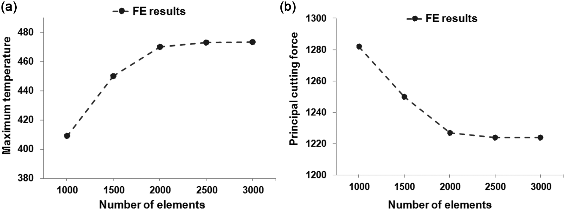
Convergence analysis on results of simulation: (a) maximum workpiece temperature and (b) principal cutting force.

After convergence analysis, to achieve steady-state mechanical conditions, the FE simulation was performed by updated Lagrangian implicit formulation and automatic remeshing technique. After that, steady-state thermal conditions were attained by one-step Eulerian simulation.^11,12 It should be noted that, material model of workpiece and contact conditions between tool and workpiece are essential inputs in simulation of the machining process that should be defined accurately.

Workpiece material modeling

Owing to the fact that in simulation of machining, large deformations with high temperatures and strains occur, the workpiece material model should satisfactorily represent plastic and thermo-mechanical behavior of workpiece deformations that are observed during the machining process. Several material models such as Johnson–Cook’s (J-C) constitutive equation (equation (1)) have been used for representation of material behavior with consideration of strain, strain rate, and temperature effects.¹³

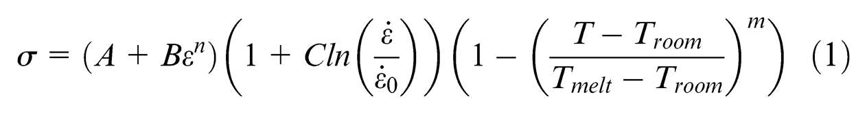
σ = (A + B ε^{n}) (1 + Cln (\frac{\overset{\cdot}{ε}}{{\overset{\cdot}{ε}}_{0}})) (1 - {(\frac{T - T_{room}}{T_{melt} - T_{room}})}^{m})

(1)

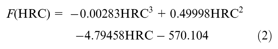
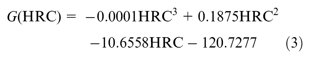
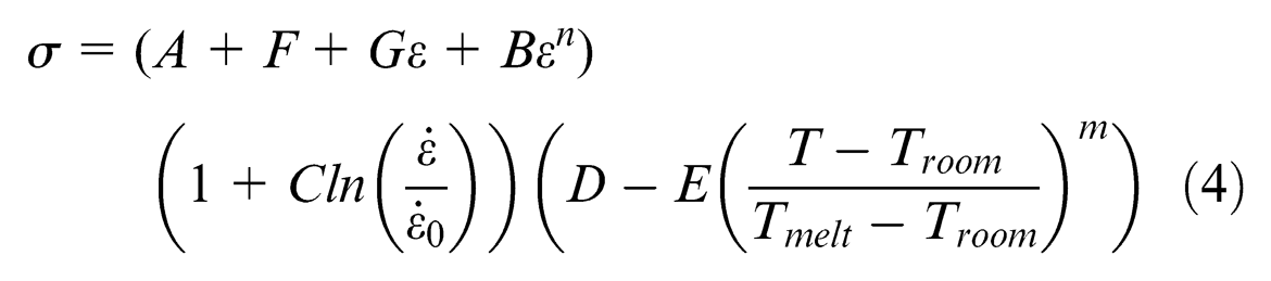
In equation (1), ε is the plastic strain, $\overset{\cdot}{ε}$ is the strain rate, ${\overset{\cdot}{ε}}_{0}$ is the reference plastic strain rate, T (°C) is the workpiece temperature, T_m is the melting temperature of the workpiece material, and T_room is the room temperature. A, B, C, n, and m are material constants as well.

However, since workpiece hardness has a critical role in material behavior, developing numerical models of hard turning is more difficult than conventional turning models. Hence, an accurate flow stress model, which presents the behavior of the material in high hardness, is necessary for simulation of hard turning.¹⁴ Hence, a new material model (for AISI H13 die steel) was introduced by Umbrello et al.¹⁴ In this model, the hardness of workpiece is incorporated in the flow stress. Based on this, F and G constants are related to the material hardness and are added to the reference J-C constitutive equation at 46HRC. The flow stress model for AISI H13 die steel at a different initial hardness is illustrated as follows

\begin{matrix} F (HRC) = - 0.00283 HR C^{3} + 0.49998 HR C^{2} \\ - 4.79458 HRC - 570.104 \end{matrix}

(2)

\begin{matrix} G (HRC) = - 0.0001 HR C^{3} + 0.1875 HR C^{2} \\ - 10.6558 HRC - 120.7277 \end{matrix}

(3)

σ = (A + F + G ε + B ε^{n}) (1 + Cln (\frac{\overset{\cdot}{ε}}{{\overset{\cdot}{ε}}_{0}})) (D - E {(\frac{T - T_{room}}{T_{melt} - T_{room}})}^{m})

(4)

In a similar research, another hardness-based flow stress (for AISI H13 die steel) was introduced by Yan et al.¹⁵ In this model, C and D constants are the functions of the workpiece hardness that are added to the reference flow stress. The mentioned model is illustrated as follows

C (HRC) = 0.0576 HR C^{2} - 3.7861 HRC - 52.82

(5)

D (HRC) = 0.6311 HR C^{2} - 12.752 HRC - 727.5

(6)

σ = (A + B ε^{- n} + Cln (ε_{0} + ε) + D) (1 + Eln (\frac{\overset{\cdot}{ε}}{{\overset{\cdot}{ε}}_{0}})) (1 - {(\frac{T - T_{room}}{T_{melt} - T_{room}})}^{m})

(7)

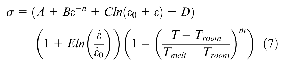
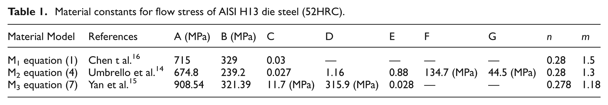
In this article, three flow stress material models were employed for simulation of hardened die steel AISI H13 (52HRC). The material constants of the flow stresses are shown in Table 1.

Table 1.

Material constants for flow stress of AISI H13 die steel (52HRC).

Material Model	References	A (MPa)	B (MPa)	C	D	E	F	G	n	m
M₁ equation (1)	Chen t al.¹⁶	715	329	0.03	—	—	—	—	0.28	1.5
M₂ equation (4)	Umbrello et al.¹⁴	674.8	239.2	0.027	1.16	0.88	134.7 (MPa)	44.5 (MPa)	0.28	1.3
M₃ equation (7)	Yan et al.¹⁵	908.54	321.39	11.7 (MPa)	315.9 (MPa)	0.028	—	—	0.278	1.18

Chip–tool contact conditions

In addition to the material model, among parameters that are considered for FE simulation, frictional and thermal conditions on the chip–tool interface play an important role in the results of simulation. In this regard, some researches on different friction models based on the existence of sticking and sliding regions on chip–tool interface have been performed, in which shear friction factor (m) and coulomb friction factors (µ) are considered for sticking and sliding region, respectively.¹⁷ Besides, global heat-transfer coefficient (h) plays an important role in temperature evolution on the chip–tool and workpiece–tool interfaces. Hence, in a few performed studies by researchers, dependence of (h) coefficient on temperature and pressure on the tool–workpiece interface was calculated through an inverse procedure.¹¹

Since implementation of the above-mentioned methods are time-consuming and difficult, several researchers have applied constant coefficients of m (or µ) and h in their simulations for describing contact conditions during the machining process.¹⁸ However, this method can lead to noticeable simulation errors. Therefore, some other researchers have employed a trial and error approach during fine-tuning contact conditions for calibrating FE simulation outputs.⁵ This approach generally leads to satisfactory results.¹⁹

Model validation

In this section, the predicted results, such as cutting forces and maximum chip surface temperature, were validated by comparing with experimental results from literature.²⁰ Validation was performed on the AISI H13 die steel (52HRC) at a feed rate of 0.25 mm/rev and cutting speed of 75, 150, and 200 m/min. In addition, the cutting tool was considered as a PCBN material with a rake angle of −5°, clearance angle of 5°, and chamfered edge of (20°) × (0.2) mm for accessing the utilized material properties of the tool and workpiece.¹⁵

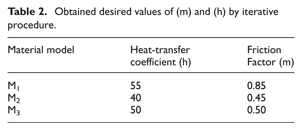
Previously, Ozel¹⁸ simulated hard turning process of AISI H13 die steel (55HRC) with constant friction coefficient and ordinary material model, which finally showed noticeable differences between the measured and simulated forces (especially at the higher cutting speeds). As he concluded, this problem probably took place because of inadequate friction modeling and limitation in the material model. However, in few of the performed studies, an efficient method was introduced to reduce simulation errors due to the turning process.¹⁹ In this method, an iterative procedure was executed for choosing the most suitable material model and determining suitable friction coefficient. Also, in another research, this iterative procedure was carried out properly for predicting temperature and cutting forces of turning process by calibrating thermal and frictional coefficients (m and h values).¹⁴ According to the mentioned points, in this study, in order to reduce simulation errors of hard turning process of AISI H13 die steel (52HRC), a new iterative procedure was used. In this method, in addition to calibrating thermal and frictional coefficients, three material models including two different hardness-based flow stresses and one ordinary flow stress were utilized. Relying on this, validation of predicted results were implemented by material models of M₁, M₂, and M₃, and for each material model, the iterative procedure was used in order to determine the suitable shear friction factor (m) and global heat-transfer coefficient (h). This iterative procedure and obtained values of m and h are shown in Table 2 and Figure 2, respectively. Also, predicted results of each model at the different cutting speeds and corresponding experimental results are given in Figure 3.

Table 2.

Obtained desired values of (m) and (h) by iterative procedure.

Material model	Heat-transfer coefficient (h)	Friction Factor (m)
M₁	55	0.85
M₂	40	0.45
M₃	50	0.50

Figure 2.

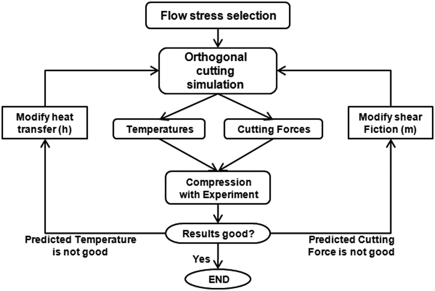
Iterative procedure for determining controllable parameters of simulation.

Figure 3.

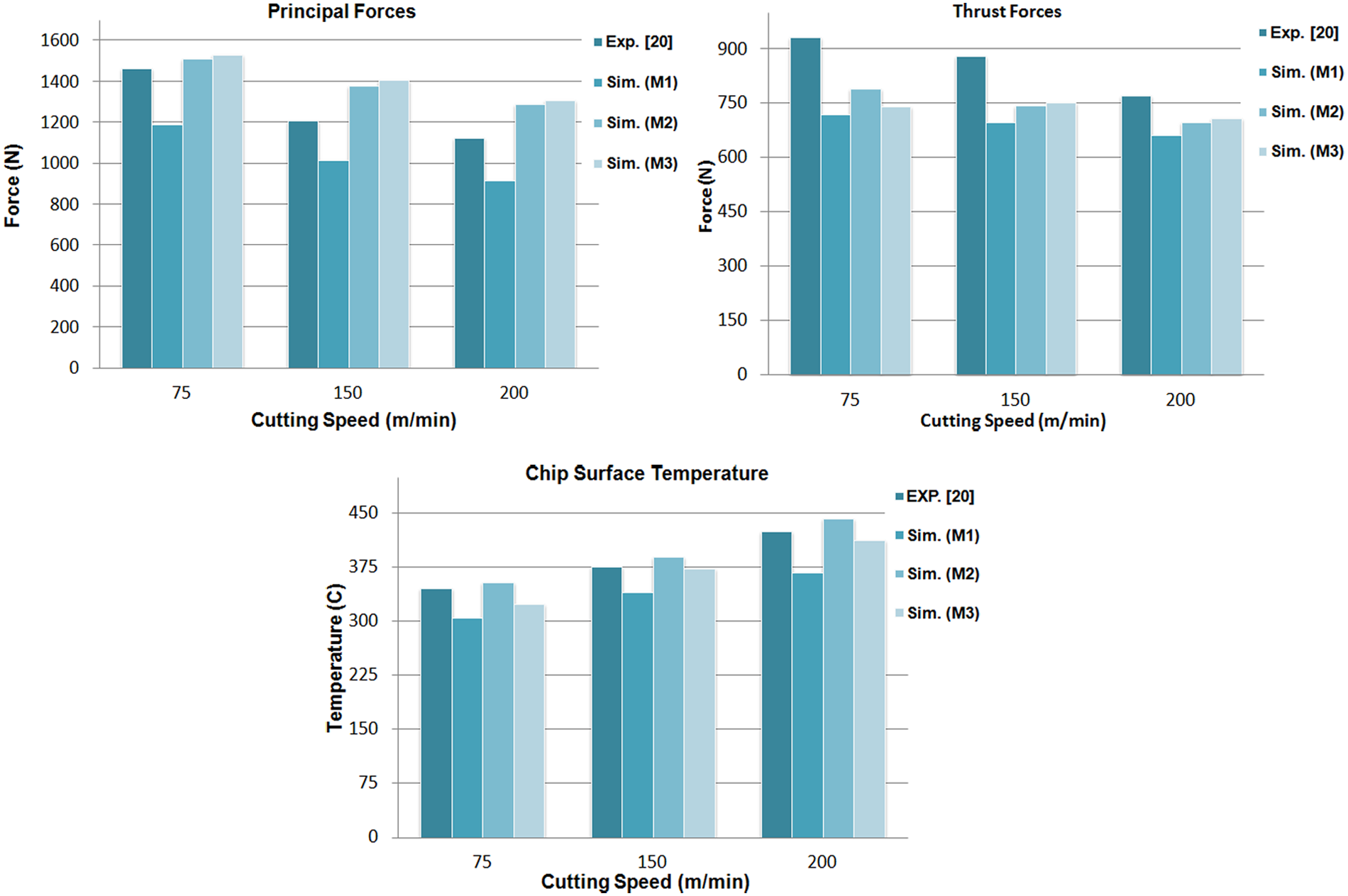
Comparison between predicted results of simulation and experimental results of literature.

As shown in Figure 3, differences between predicted and experimental results are approximately slight when hardness-based flow stresses of M₂ and M₃ are considered, but these differences are increased when ordinary flow stress of M₁ is employed. Therefore, both hardness-based flow stresses of M₂ and M₃ can be used properly for hard turning simulation of AISI H-13 (52HRC). Hence, in the rest of the article, one of these (flow stress of the M₃ with h = 50 and m = 0. 5) was chosen for subsequent simulations. Figure 4 shows the steady-state thermal conditions during FE simulation of orthogonal turning at the cutting speed of 200 m/min (with considering three different material models). As shown in this figure, by applying the material models of M₂ and M₃ for simulation of turning process (see Figure 4(b) and (c)), predicted temperature is more near the experiment than when material model of M₁ is employed (see Figure 4(a)).

Figure 4.

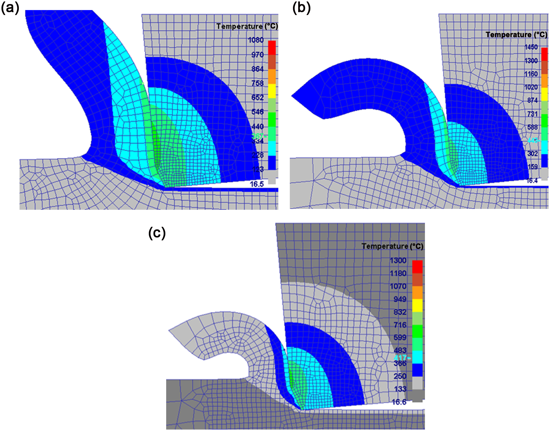
Simulation of temperature distribution during orthogonal turning at the cutting speed of 200 m/min by material model: (a) M₁, (b) M₂, and (c) M₃

Numerical results

After validation stage and choosing the desired controllable parameters of simulations, numerical investigations were performed in order to evaluate thermo-mechanical loads. In this regard, the effect of machining parameters such as cutting speed, feed rate, chamfer angle (∅), chamfer width (W) and rake angle (γ) were evaluated on the effective strain and temperature of the workpiece during the orthogonal turning process.

Owing to the fact that each of the above-mentioned parameters is considered in four levels, the total numbers of possible simulations (testing conditions) are extremely high. To solve this problem, design of the experiment based on the Taguchi method was utilized. This method uses a special design of orthogonal arrays to study the entire possible space with only a small numbers of experiments that contains a chosen subset of all testing conditions.⁴ In this study, (L₃₂) orthogonal array in Taguchi method was considered in order to determine the desired testing conditions. The details of the machining parameters, testing conditions, and obtained results of FE simulation are given in Table 3.

Table 3.

Predicted results of simulation during orthogonal turning.

Number	V _{C (m/min)}	F _(mm/rev)	γ_(degree)	W _(mm)	∅_(degree)	Workpiece temperature (°C)	Workpiece effective strain
1	150	0.10	0	0.10	15	151	0.73
2	150	0.15	−5	0.15	20	219	0.94
3	150	0.20	−10	0.20	25	339	1.41
4	150	0.25	−15	0.25	30	495	1.69
5	200	0.10	−0	0.15	20	184	0.86
6	200	0.15	−5	0.10	15	173	0.73
7	200	0.20	−10	0.25	30	502	1.86
8	200	0.25	−15	0.20	20	410	1.24
9	250	0.10	−5	0.20	30	382	1.93
10	250	0.15	0	0.25	25	265	1.07
11	250	0.20	−15	0.10	20	293	1.09
12	250	0.25	−10	0.15	15	287	0.91
13	300	0.10	−5	0.25	25	276	1.32
14	300	0.15	0	0.20	30	367	1.24
15	300	0.20	−15	0.15	15	360	1.06
16	300	0.25	−10	0.10	20	279	0.97
17	150	0.10	−15	0.10	30	358	1.71
18	150	0.15	−10	0.15	25	316	1.39
19	150	0.20	−5	0.20	20	234	1.14
20	150	0.25	0	0.25	15	219	0.71
21	200	0.10	−15	0.15	25	367	1.82
22	200	0.15	−10	0.10	30	282	1.29
23	200	0.20	−5	0.25	15	209	0.93
24	200	0.25	0	0.20	20	240	0.91
25	250	0.10	−10	0.20	15	242	1.04
26	250	0.15	−15	0.25	20	415	1.55
27	250	0.20	0	0.10	25	254	0.81
28	250	0.25	−5	0.15	30	356	1.09
29	300	0.10	−10	0.25	20	287	1.24
30	300	0.15	−15	0.20	15	402	1.40
31	300	0.20	0	0.15	30	346	1.18
32	300	0.25	−5	0.10	25	301	0.89

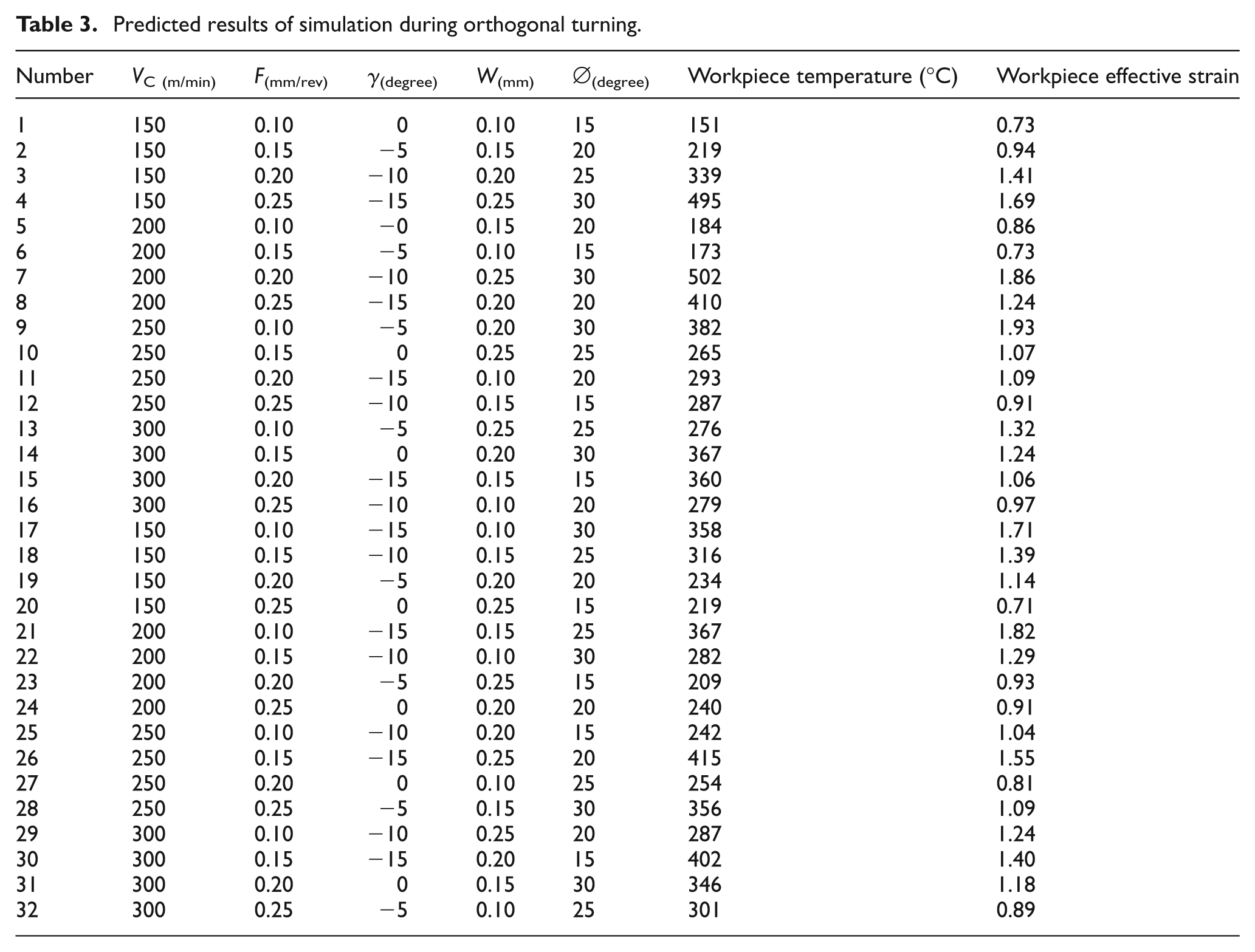
In the following sections, the obtained results of Table 3 are applied to the intelligent methods.

Artificial intelligent

Intelligent methods based on the predictive and optimization methods have been significantly developed and utilized in several fields such as mechanical engineering.²¹ In the rest of the article, after briefly explaining some basic intelligent methods, these aims have been pursued by utilizing some programs under MATLAB software.

Genetic algorithm

Genetic algorithm (GA), which is derived from nature (human’s genetic), is a well-known population-based algorithm used to find optimal solutions.²² Any member of population is called a chromosome and consists of genes equal to the optimization variables of the problem. In every generation, all the chromosomes are evaluated by objective function, and based on their fitness, fitter chromosomes are produced in the next generation. Finally, after some iterations, the algorithm converges toward the optimal solution.

MOO

Many real-life optimization problems are not limited to the optimization of one single objective, therefore for solving them two or more conflicting objectives are required to be optimized at the same time. Normally, for these problems, a single solution cannot be found that simultaneously optimizes all the objectives. While searching for solutions, one reaches points such that, when attempting to increase an objective, other objectives will be decreased as a result.²³ Therefore, MOO can be defined as the process of simultaneously optimizing two or more conflicting objectives, and it can be found in many fields wherever optimal decisions need to be taken in the presence of trade-offs between two or more conflicting objectives. In MOO problems, there are two spaces: decision and objective spaces. With regard to the first, decision space includes input variables of problem, while the second space includes output values of the problem. Since output variables are related to the particular input values, the main goal of optimization problems is allocated to find the optimal input variables in order to minimize/maximize corresponding objective values.²³

The fitness evaluation in MOO is different from single-objective optimization, and there are a set of optimal solutions that dominate other solutions in the decision space. For example, in minimization problems, a feasible solution X is said to dominate other feasible solutions y, if and only if, z_i(x) ≤ z_i(y) for I = 1, …, m and z_j(x)<z_j(y) for at least one objective function j. In this condition, the set of all feasible nondominated solution in X space is said to be Pareto-optimal, and the corresponding objective function values in objective space is called Pareto front.^23,24 Also, all solution sets in the Pareto front are not absolutely better than other solutions in the Pareto front. In fact, each solution is better than other solutions at least in one objective.

The final goal of MOO algorithms is to identify solutions in the Pareto-optimal set. One of the most popular evolutionary algorithms for solving MOO problems is the nondominated GA (NSGA-II). It is an extension of the simple GA to a nondominated sorting version of candidate solutions (Pareto-optimal points) in order to solve multiobjective problems.²⁴

ANN

ANNs are capable of estimating complex nonlinear relationships between input-machining parameters and corresponding outputs. In this study, cutting speed, feed rate, chamfer angle, chamfer width, and rake angle are considered as inputs to neural network, and temperature or effective strain is predicted as an output of network. Each network is composed of several neurons at different layers, and each neuron is affected by bias and transfer functions. Owing to the fact that neurons of each neural network are connected to each other by weighted connection links, by setting transfer functions and adjusting weights and biases of each neural network, the outputs of the turning process can be estimated properly. Figure 5(a) shows the schematic view of a neuron considering corresponding weights, bias, and transfer function, and Figure 5(b) shows an example of a multilayer perception NN that was employed in order to predict turning outputs.

Figure 5.

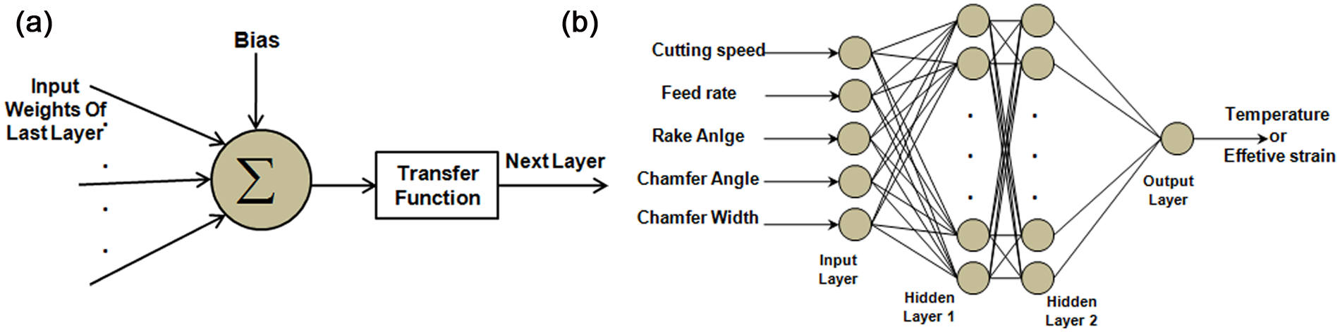
(a) Schematic view of a neuron and (b) structure of an artificial multilayer perception neural network.

Training ANN by GA

Previously, different methods were utilized to train neural networks of which most of them use mathematical methods such as back propagation.²⁵ Recently, some researchers have presented a new efficient method in order to train NN, in which weights and biases of neural networks are updated by GA.²² In this method, initial network topology is a multilayer perception neural network in which none of the conventional training methods have been considered.

In the mentioned method, weights and biases of neural network are the variables of GA. The flowchart of training the ANN by GA is shown in Figure 6.

Figure 6.

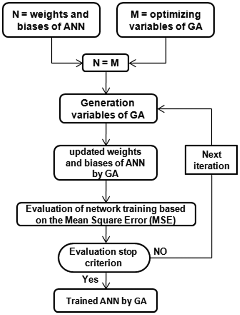
Training of the ANN by GA.

During network training, testing and training errors are gradually decreased until specific number of iterations, which depend on the network capacity; after passing these iterations, the testing error will no more be decreased. In this stage, it is called that the network has been overtrained, which leads to increase in testing error and decrease in network performance. Therefore, by using the training of the ANN by GA, it is possible to obtain the most suitable iteration for training the network and prevent overtraining of the NN by controlling testing error in different iterations of GA.

Leave-one-out cross-validation method

Cross-validation is one of the most important and effective approaches used for verification of models in statistical machine learning in order to estimate how well a predictive model we have learned from training data is going to perform on the future unseen (test) data. This method is usually used when the number of training and testing data is not very large or it is too difficult to create large training/testing dataset for learning of the model. In this method, in each iteration, one sample of the data point is temporarily considered as a validation data, and the remaining data are used for the training of the model. After training the model, prediction error is calculated based on the validation data. If the original training data have K samples, this procedure repeated K times (equal to the number of observations in the original training set). After that, average of these errors is reported as the prediction error of our predictive model on the whole dataset. As seen, in this validation approach, during K iterations, all the samples have the chance to act as a training sample and testing sample.²⁶

Obtained results

The obtained results in this part are divided into two subdivisions. The first subdivision is allocated to present a precise model for predicting the maximum temperature and effective strain of workpiece by using two discrete NNs that are divided into two parts: choosing the best structure of neural network and training the chosen network structure. The second subdivision is allocated to simultaneous optimization of thermo-mechanical loads during orthogonal turning operation. This subdivision is also divided into two parts: simultaneous optimization of the process by NSGA-II and evaluation of obtained results of NSGA-II by performing FE simulation for some of the obtained results.

Prediction of effective strain and temperature by ANN

Usually, the amount of available data for training and testing the neural networks is not much at the manufacturing processes. Therefore, applying a suitable method for network training plays an important role in order to increase the performance and efficiency of the method. But usually, customary training methods have been implemented to the performed researches at the manufacturing processes.²⁵ Hence, we employed and also developed an efficient method in our work. This method, which is based on training the NNs by GA and its combination with leave-one-out cross-validation (LOOCV) method, is a suitable method despite less training data.

First, the best structure of ANNs was determined by the LOOCV method. In this method, 31 rows of data and one datum were selected for training and testing the network, respectively, from data samples of the Table 3. Then, training operations of the network were carried out by GA. Besides, this operation was repeated 31 times and each time a new data sample was selected as a testing data while training process was performed on the 31 remaining data. Then, the average of the absolute error of the 32 iterations was considered as network error. Figure 7 shows the flowchart of the applied method.

Figure 7.

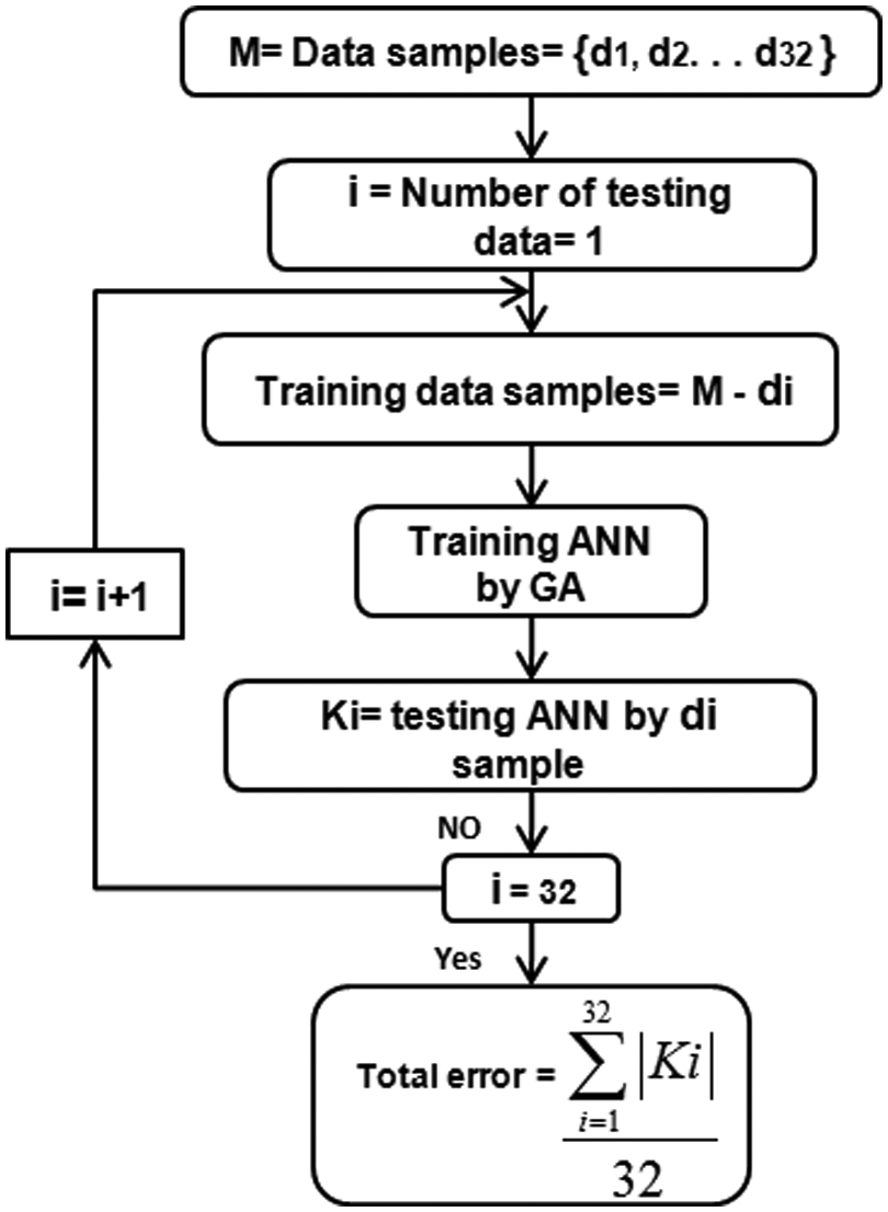
Leave-one-out cross-validation method for choosing network structure.

The mentioned method was repeated three times on the different structures of NN and, at the end, the average of the obtained errors was considered as error of each network. These results were reported in Table 4. The obtained results showed that NNs with the structure of 5-5-3-1 and 5-6-4-1 are the best structures for predicting the maximum temperature and effective strain of workpiece, respectively. It should be noted that, the all input and output data were normalized linearly between 0 and 1 in order to improve training process, and also transfer functions of purline and tansig were considered empirically for output and hidden layers of neural networks, respectively. Some of the adjusted parameters of GA include population size of 135, elite count of 8, iteration of 100, migration fraction of 0.7, and migration interval of 6.

Table 4.

Choosing the best structure of the ANNs by leave-one-out cross-validation method.

Structure of ANN	5-12-3-1	5-9-4-1	5-6-4-1	5-5-3-1	5-3-2-1	5-4-3-1	5-12-1	5-7-1	5-3-1
Temperature (%)	11	13	9	7	8	9	18	21	24
Effective strain (%)	12	8	7	9	13	12	23	19	16

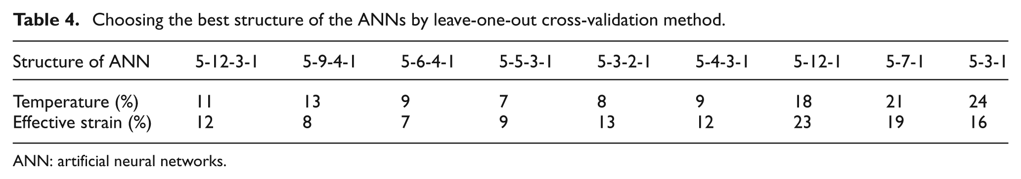
ANN: artificial neural networks.

After selecting the suitable structure, the NNs should be trained. For this propose, the GA was employed for training the two chosen networks by applying 27 rows of training data and 5 rows of testing data from data samples of the Table 3. Also, the training process was carried out in different iterations of GA to prevent overtraining. At the end, the neural networks were trained excellently for predicting the maximum temperature and effective strain of the workpiece by trial and error procedure and by changing the iterations of GA. The obtained results for each network is shown in Table 5. Also, Figure 8 shows convergence diagram of GA for training the NNs.

Table 5.

Final errors of the ANNs trained by GA.

ANN	GA iteration	MSE training error	Mean training error	Absolute testing error	Mean testing error
Temperature	900	0.00121	2.8%	1.2%–5.3%–4.9%–4.9%–1.9%	3.7%
Effective strain	1500	0.00057	1.7%	0.5%–2.4%–2.5%–4.2%–6.1%	3.2%

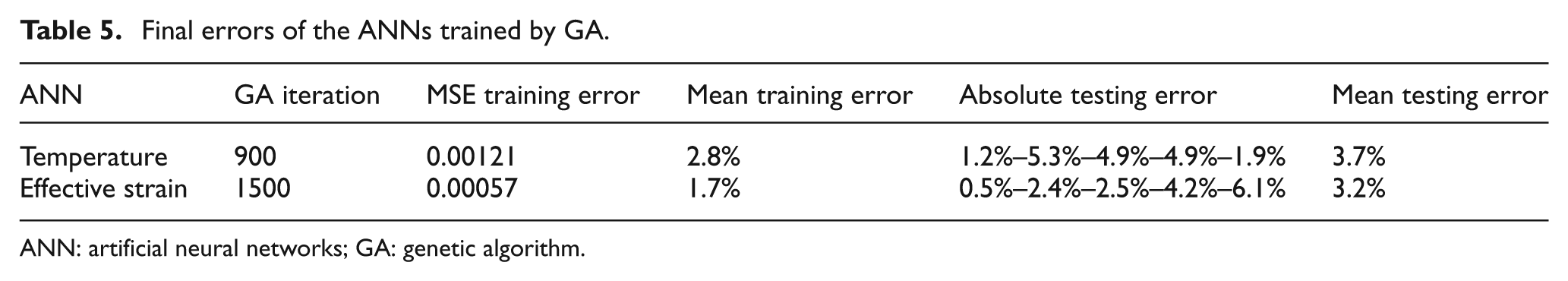
ANN: artificial neural networks; GA: genetic algorithm.

Figure 8.

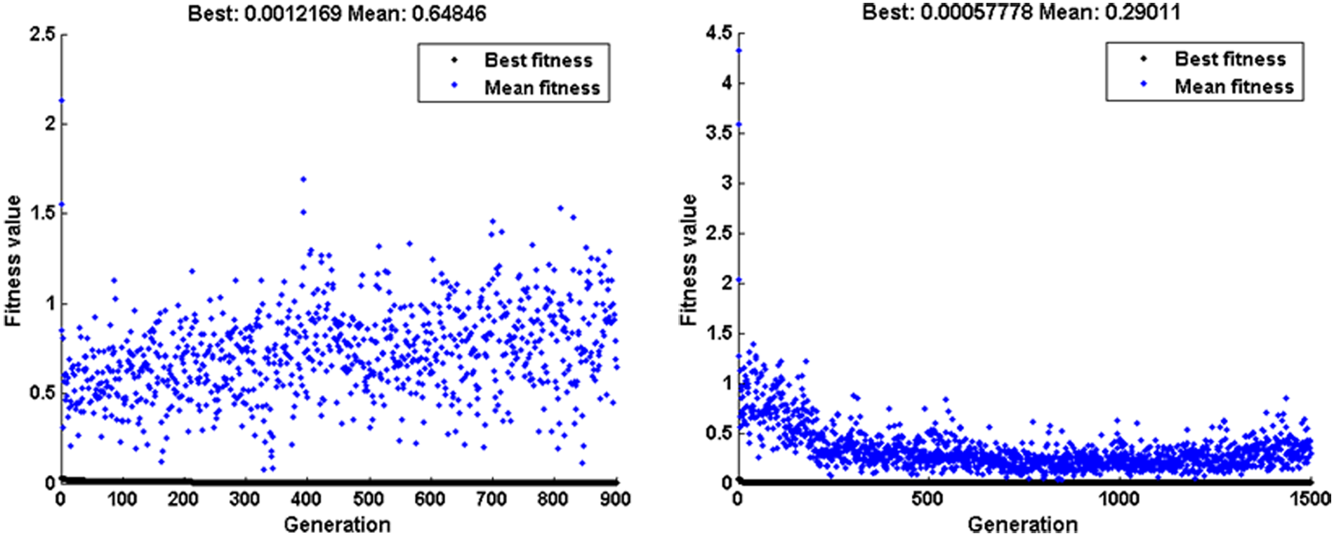
Convergence curves of training procedure for temperature and effective strain.

Simultaneous optimization of thermo-mechanical loads

In this section, to access the desired surface properties of the machined workpiece, thermo-mechanical loads were optimized during the hard turning process. Here, suitable machining conditions were determined by MOO algorithm (NSGA-II) in order to simultaneously minimize the temperature and maximize effective strain of the workpiece. Therefore, the objective functions that were considered for NSGA-II are as follows

Objective 1 = Workpiece temperature

(8)

Objective 2 = \frac{1}{Workpiece effective strain}

(9)

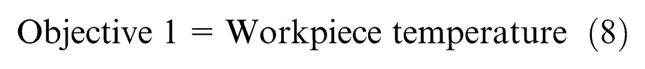
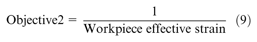
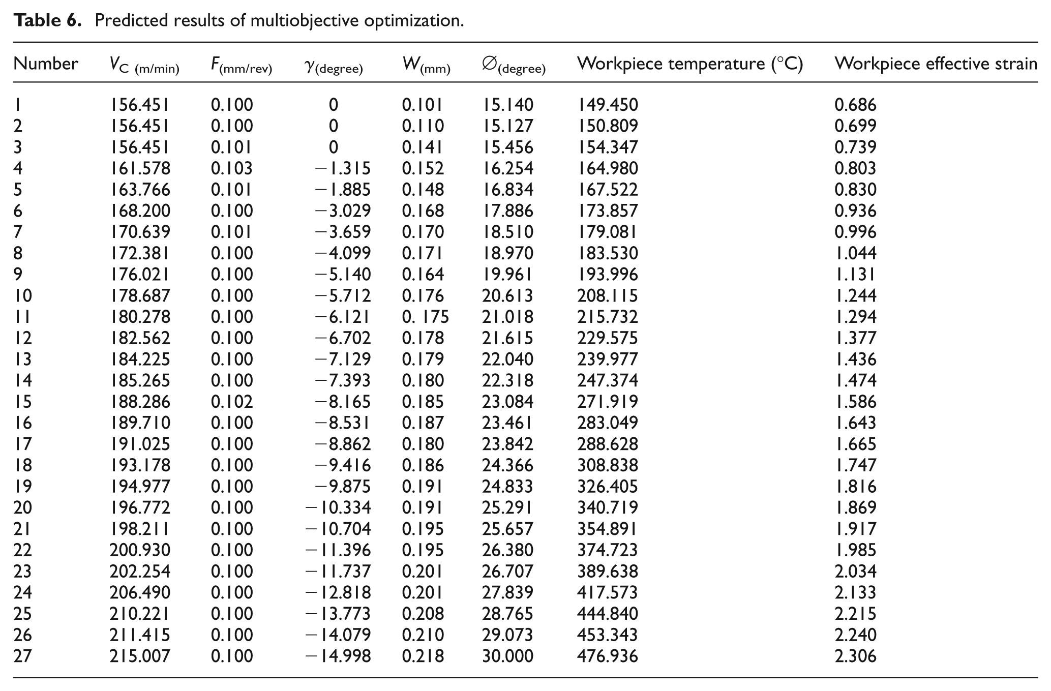
The functions implemented by NNs in the previous section were utilized as objective functions of NSGA-II. By doing this, NSGA-II determined the optimal Pareto-front by searching the decision space (input-machining parameters) and sorting the nondominated solutions (based on the minimizing temperature and maximizing effective strain). Some adjusted parameters of NSGA-II include crossover probability of 0.8, mutation probability of 0.25, population size of 90, and iteration of 1000. The optimal Pareto-front (nondominated solution set) that was obtained after optimization procedure is shown in Figure 9. Also, a set of 27 solutions (of 90 obtained solutions) and corresponding decision variables (machining parameters) were sorted based on the increasing temperature and were reported in Table 6. As can be seen, by moving to lower solution sets in this table, the state of objective 1 becomes worse while objective 2 becomes better. Since neither of the solution sets is absolutely better than the other (not dominated by each other), both are not the optimal solution that can be selected according to the requirement of the process engineer.

Figure 9.

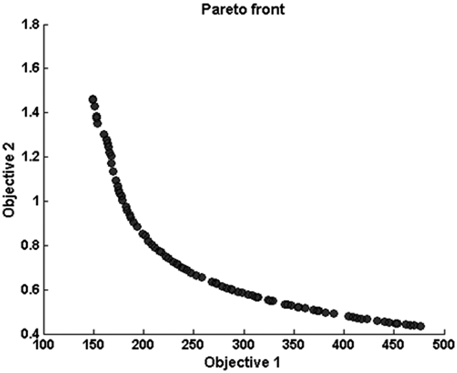
Optimal Pareto-front.

Table 6.

Predicted results of multiobjective optimization.

Number	V _{C (m/min)}	F _(mm/rev)	γ_(degree)	W _(mm)	∅_(degree)	Workpiece temperature (°C)	Workpiece effective strain
1	156.451	0.100	0	0.101	15.140	149.450	0.686
2	156.451	0.100	0	0.110	15.127	150.809	0.699
3	156.451	0.101	0	0.141	15.456	154.347	0.739
4	161.578	0.103	−1.315	0.152	16.254	164.980	0.803
5	163.766	0.101	−1.885	0.148	16.834	167.522	0.830
6	168.200	0.100	−3.029	0.168	17.886	173.857	0.936
7	170.639	0.101	−3.659	0.170	18.510	179.081	0.996
8	172.381	0.100	−4.099	0.171	18.970	183.530	1.044
9	176.021	0.100	−5.140	0.164	19.961	193.996	1.131
10	178.687	0.100	−5.712	0.176	20.613	208.115	1.244
11	180.278	0.100	−6.121	0. 175	21.018	215.732	1.294
12	182.562	0.100	−6.702	0.178	21.615	229.575	1.377
13	184.225	0.100	−7.129	0.179	22.040	239.977	1.436
14	185.265	0.100	−7.393	0.180	22.318	247.374	1.474
15	188.286	0.102	−8.165	0.185	23.084	271.919	1.586
16	189.710	0.100	−8.531	0.187	23.461	283.049	1.643
17	191.025	0.100	−8.862	0.180	23.842	288.628	1.665
18	193.178	0.100	−9.416	0.186	24.366	308.838	1.747
19	194.977	0.100	−9.875	0.191	24.833	326.405	1.816
20	196.772	0.100	−10.334	0.191	25.291	340.719	1.869
21	198.211	0.100	−10.704	0.195	25.657	354.891	1.917
22	200.930	0.100	−11.396	0.195	26.380	374.723	1.985
23	202.254	0.100	−11.737	0.201	26.707	389.638	2.034
24	206.490	0.100	−12.818	0.201	27.839	417.573	2.133
25	210.221	0.100	−13.773	0.208	28.765	444.840	2.215
26	211.415	0.100	−14.079	0.210	29.073	453.343	2.240
27	215.007	0.100	−14.998	0.218	30.000	476.936	2.306

To confirm that suitable interaction takes place between FEM and MOO, some FE simulations were carried out according to the machining parameters of Table 6. In this regard, Figure 10 shows the comparison between predicted results of FE simulation and obtained results of NSGA-II. As shown in this figure, simulation results are very near the corresponding results of MOO, and there is good agreement between these methods. Hence, it can be said that the proposed hybrid technique of FEM–ANN–MOO in this article was implemented successfully. In fact, by employing this hybrid technique, suitable machining parameters were determined in order to optimize thermo-mechanical loads during hard turning process, while these results were not obtained by using previous simulations. Figure 11 shows distribution of temperature and effective strain on workpiece during turning process with machining parameters of solution set of 21 and 27. As shown in this figure, in each test, the conditions of thermal loads and mechanical loads is not better than the other, and it is based on the definition of MOO.

Figure 10.

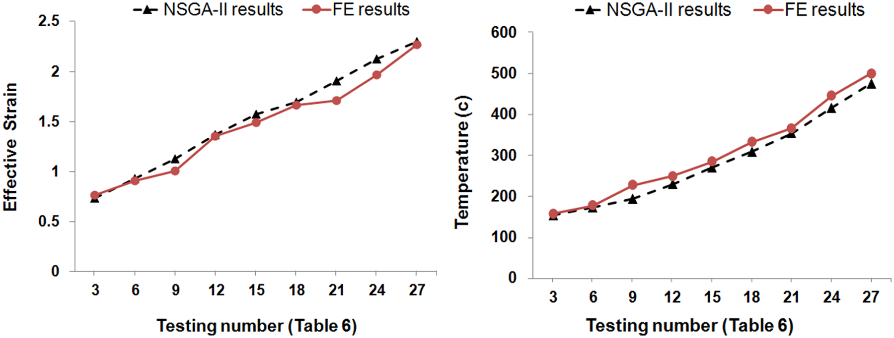
Comparison between the obtained results of NSGA-II and predicted results of FE simulation.

Figure 11.

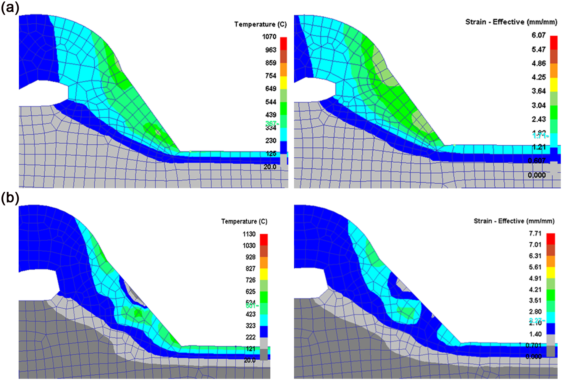
Distribution of temperature and effective strain with machining parameters of Table 6: (a) solution set of 21 and (b) solution set of 27.

Conclusion

The main objective of this article is to develop a useful and new hybrid method based on the FEM–ANN–MOO in order to predict and optimize thermo-mechanical loads during the orthogonal turning of AISI H13-hardened die steel. It is possible to state as follows:

By doing iterative procedure, it was found that the material model has more significant effects on calibration of simulation results than contact conditions. Moreover, it was found that using hardness-based flow stress is necessary for accurate simulation of hard turning process.

The new efficient method was employed to present a predictive model of the hard turning process by ANNs. At first, suitable structures of neural networks were determined by LOOCV method; then training of selected networks was carried out by GA. Although these methods were time-consuming in programming and computations, applied methods lead to an increase in accuracy and effectiveness of the neural networks in spite of less training data. In this regard, testing error ranges were obtained between 0.5% and 6.1% for both the ANNs.

Some FE simulations were performed with the same machining parameters obtained by NSGA-II. Comparison between results of NSGA-II and results of FE simulation showed that there were very good agreement between FE and intelligent methods employed in this article.

Optimal solution set of Table 6 showed that in order to achieve simultaneous optimization of thermo-mechanical loads in a specific range of investigated input parameters, the feed rate was kept at a minimum rate (0.1 mm/rev). Besides, it was found that cutting speed, rake angle, chamfered width, and chamfer angle were between 156 and 215 m/min, 0° and 15°, 0.1 and 0.021 mm, and 15° and 30°, respectively, on increasing each of which the state of mechanical loads was improved and the state of thermal loads deteriorated.

In this study, 2D analysis was employed for turning simulation, while 3D simulation of turning process is more realistic than 2D simulation and the effect of more machining parameters can be investigated. Besides, number of two outputs of the process were optimized, while developing MOO algorithm is required for simultaneously optimizing more than two outputs of the process. Finally, it should be said that the implemented hybrid technique in this study can be applied appropriately to other branches of mechanical engineering as well.

Footnotes

Funding

This research received no specific grant from any funding agency in the public, commercial, or not-for-profit sectors.

Conflict of interest

The authors of this article declare that there is no conflict of interest.

References

Davim

. Machining fundamental and recent advances. 1st ed. New York: Springer, 2008, pp.57–124.

Farid

Sharif

Idris

. Surface integrity study of high-speed drilling of Al–Si alloy using HSS drill. Proc IMechE, Part B: J Engineering Manufacture 2011; 225: 1001–1007.

Razfar

Zanjani Zadeh

. Optimum damage and surface roughness prediction in end milling glass fibre-reinforced plastics, using neural network and genetic algorithm. Proc IMechE, Part B: J Engineering Manufacture 2009; 223: 653–664.

Yang

Sheu

. Optimal machining parameters in the cutting process of glass fibre using the reliability analysis based on the Taguchi method. Proc IMechE, Part B: J Engineering Manufacture 2008; 222: 1075–1082.

Özel

. Computational modelling of 3D turning: influence of edge micro-geometry on forces, stresses, friction and tool wear in PcBN tooling. J Mater Process Technol 2009; 209: 5167–5177.

Yang

. Prediction of maximum forming load and billet dimensions using an abductive network and finite element method simulation of a near net-shaped helical gear forging. Proc IMechE, Part B: J Engineering Manufacture 2009; 223: 289–304.

Umbrello

Ambrogio

Filice

. An ANN approach for predicting subsurface residual stresses and the desired cutting conditions during hard turning. J Mater Process Technol 2007; 189: 143–152.

Umbrello

Ambrogio

Filice

. A hybrid finite element method—artificial neural network approach for predicting residual stresses and the optimal cutting conditions during hard turning of AISI 52100 bearing steel. Mater Des 2008; 29: 873–883.

Davim

. Machining of hard material. 1st ed. New York: Springer, 2011, pp.115–172.

10.

Gadalaa

Movahhedy

Wang

. On the mesh motion for ALE modeling of metal forming processes. Finite Elem Anal Des 2002; 38: 435–459.

11.

Ceretti

Filice

Umbrello

. ALE simulation of orthogonal cutting: a new approach to model heat transfer phenomena at the tool–chip interface. CIRP Ann-Manuf Techn 2007; 56: 69–72.

12.

Deform 2D V9.0.1. User Manual. Columbus, OH: Scientific Forming Technologies Corporation, 2006.

13.

Johnson

Cook

. Fracture characteristics of three metals subjected to various strains strain rates temperatures and pressures. Eng Fract Mech 1985; 21: 31–48.

14.

Umbrello

Rizzuti

Outeiro

. Hardness-based flow stress for numerical simulation of hard machining AISI H13 tool steel. J Mater Process Technol 2008; 199: 64–73.

15.

Yan

Hua

Shivpuri

. Flow stress of AISI H13 die steel in hard machining. Mater Des 2007; 28: 272–277.

16.

Chen

EI-Wardany

Nasr

. Effects of edge preparation and feed when hard turning a hot work die steel with polycrystalline cubic boron nitride tools. CIRP Ann-Manuf Techn 2006; 55: 89–92.

17.

Filice

Micari

Rizzuti

. A critical analysis on the friction modelling in orthogonal machining. Int J Mach Tool Manu 2007; 47: 709–714.

18.

Özel

. Modeling of hard part machining: effect of insert edge preparation in CBN cutting tools. J Mater Process Technol 2003; 141: 284–293.

19.

Umbrello

. Finite element simulation of conventional and high speed machining of Ti6Al4V alloy. J Mater Process Technol 2008; 196: 79–87.

20.

Aspinwall

Brazil

. Modeling of temperature and forces when orthogonally machining hardened steel. Int J Mach Tool Manu 1999; 39: 885–903.

21.

Soleymani Yazdi

Razfar

Asadnia

. Modelling of the thrust force of the drilling operation on PA6–nanoclay nanocomposites using particle swarm optimization. Proc IMechE, Part B: J Engineering Manufacture 2011; 225: 1757–1771.

22.

Filho

ACP

Filho

. Hybrid training approach for artificial neural networks using genetic algorithms for rate of reaction estimation: application to industrial methanol oxidation to formaldehyde on silver catalyst. Chem Eng Sci 2010; 157: 501–508.

23.

Zitzler

Laumanns

Bleuler

.A tutorial on evolutionary multiobjective optimization, in Gandibleux

Sevaux

Sorensen

T’Kindt

(Eds), Methaheuristics for Multiobjective Optimisation, Vol. 535, Lecture Notes in Economics and Mathematical Systems, Springer-Verlag, Berlin, 2004.

24.

Deb

Pratap

Agarwal

. A fast and elitist multi objective genetic algorithm: NSGA-II. IEEE T Evolut Comput 2002; 6: 182–197.

25.

Özel

Nadgir

. Prediction of flank wear by using back propagation neural network modeling when cutting hardened H-13 steel with chamfered and honed CBN tools. Int J Mach Tool Manu 2002; 42: 287–297.

26.

Ron

. A study of cross-validation and bootstrap for accuracy estimation and model selection. In: Proceedings of the fourteenth international joint conference on artificial intelligence, pp.1137–1143. Morgan Kaufmann Publishers Inc, San Francisco, CA, USA, 1995.

Integration of finite element simulation and intelligent methods for evaluation of thermo-mechanical loads during hard turning process

Abstract

Keywords

Introduction

Surface integrity in turning operation

FE simulation

Workpiece material modeling

Chip–tool contact conditions

Model validation

Numerical results

Artificial intelligent

Genetic algorithm

MOO

ANN

Training ANN by GA

Leave-one-out cross-validation method

Obtained results

Prediction of effective strain and temperature by ANN

Simultaneous optimization of thermo-mechanical loads

Conclusion

Footnotes

Funding

Conflict of interest

References