Uncertainty and Prior Assumptions,Rather Than Innate Logarithmic Encoding,Explain Nonlinear Number-to-Space Mapping

Abstract

Mapping number to space is natural and spontaneous but often nonveridical, showing a clear compressive nonlinearity that is thought to reflect intrinsic logarithmic encoding of numerical values. We asked 78 adult participants to map dot arrays onto a number line across nine trials. Combining participant data, we confirmed that on the first trial, mapping was heavily compressed along the number line, but it became more linear across trials. Responses were well described by logarithmic compression but also by a parameter-free Bayesian model of central tendency, which quantitatively predicted the relationship between nonlinearity and number acuity. To experimentally test the Bayesian hypothesis, we asked 90 new participants to complete a color-line task in which they mapped noise-perturbed color patches to a “color line.” When there was more noise at the high end of the color line, the mapping was logarithmic, but it became exponential with noise at the low end. We conclude that the nonlinearity of both number and color mapping reflects contextual Bayesian inference processes rather than intrinsic logarithmic encoding.

Humans and many other species spontaneously associate numbers with space, even in early infancy (de Hevia & Spelke, 2010; Drucker & Brannon, 2014; McCrink & Opfer, 2014; Rugani et al., 2015). Under many conditions, number-to-space mapping is nonlinear, following a logarithmic-like compression. Compressive mapping is most evident in children (Kim & Opfer, 2017) but becomes progressively more linear with schooling in neurotypical children (Dehaene et al., 2008; Kim & Opfer, 2017; Opfer & Siegler, 2007). Individuals with dyscalculia show more number-line nonlinearities than age-matched neurotypical individuals (Anobile et al., 2019; Geary et al., 2008). Adults also show compressive mapping under certain circumstances, such as lack of formal education (Dehaene et al., 2008) or deprived attentional resources (Anobile, Cicchini, & Burr, 2012; Anobile, Turi, et al., 2012; Dotan & Dehaene, 2016).

The compressive nonlinearity in the number line has been interpreted as evidence for intrinsic logarithmic processes in numerosity processing (Dehaene et al., 2008), which become more linear with education and attention. This idea finds support from the fact that physiological estimates of bandwidth of numerosity receptors increase with numerosity (Nieder, 2016) and that errors in numerosity estimation often follow Weber’s law (Anobile et al., 2014; Dehaene, 2003; Ross, 2003; Whalen et al., 1999). However, Anobile, Cicchini, and Burr (2012) suggested an alternative approach: that the nonlinearity was an example of regression to the mean (or central tendency), a universal phenomenon occurring for estimation of almost every quantity, including size, time, and number, in which responses gravitate toward the average of the response space (Hollingworth, 1910). Regression to the mean is well described within the Bayesian framework, where the mean is the prior, which combines with sensory data (the likelihood), following Bayes’s rule. The use of the mean as a prior has been shown to be an efficient strategy, reducing estimation error (Cicchini et al., 2012; Jazayeri & Shadlen, 2010).

Figure 1 shows how regression to the mean causes compressive nonlinearities in number mapping. Because the effect of the prior depends on the relative reliability (reciprocal variance) of the sensory data, it will have more of an effect at high than at low numbers because variance in numerosity judgments is known to increase with numerosity. For number-line tasks, the increase in root variance tends to follow a square-root relationship (Cicchini et al., 2014; Pomè et al., 2021), as modeled in this example. Figure 1a shows a hypothetical probability density function of the prior (black curve), together with probability density functions for the likelihoods for Numbers 6 and 24 (purple and red dashed curves, respectively). The broader distribution is influenced more than the narrow distribution when multiplied by the prior, resulting in more displacement at high than at low numbers, causing the compression observed in Figure 1b. However, this will occur only if observers are relatively imprecise; otherwise, all likelihoods will be narrow, relatively unaffected by the prior (gray curve).

Fig. 1.

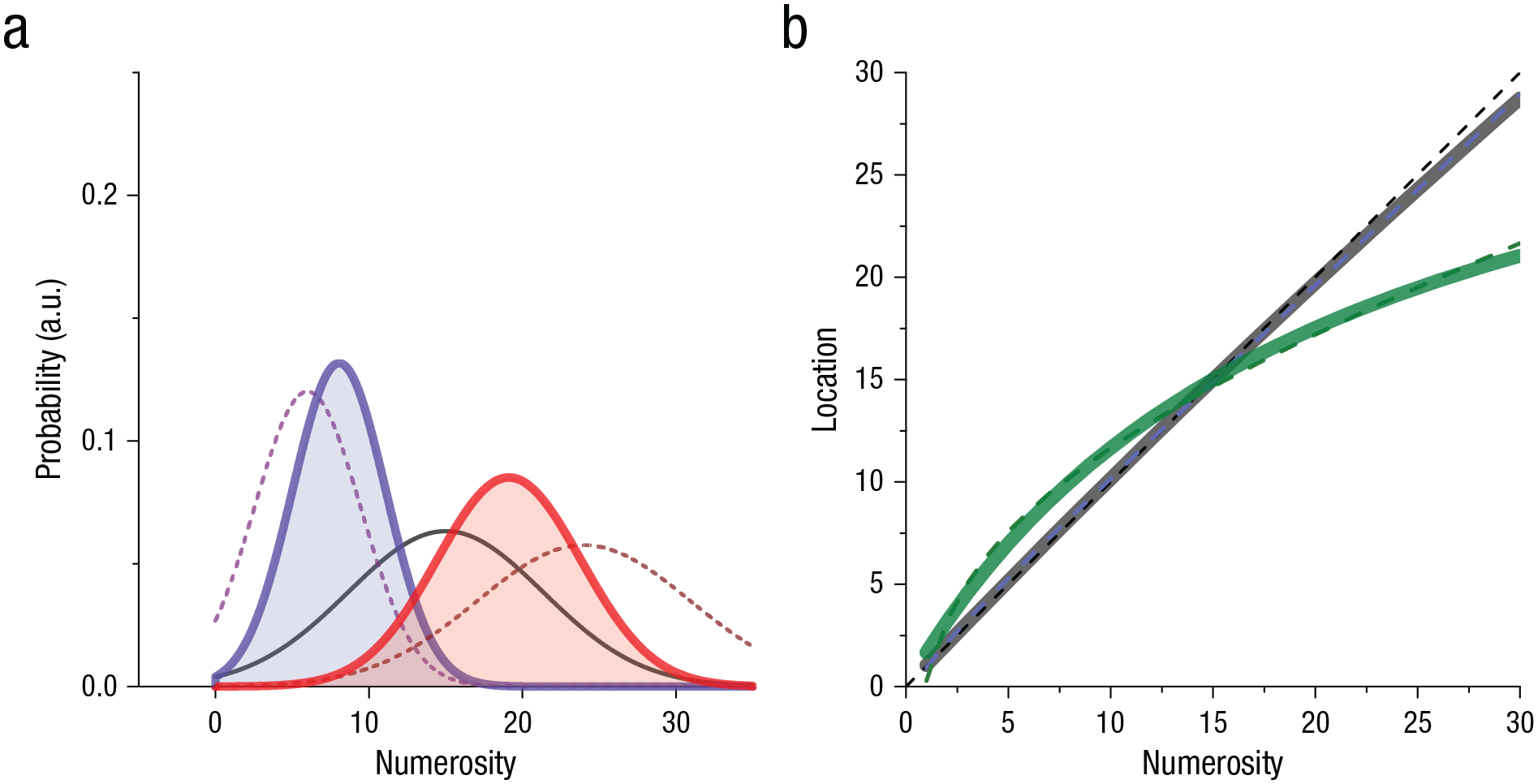
Regression to the mean within the Bayesian framework. The graph in (a) illustrates how the optimal combination of current evidence with prior knowledge is given by multiplication of the prior and likelihood distributions to yield the posterior Gaussian distribution. The prior is assumed to be centered in the middle of the number line and to have constant width ( ${\sigma }_p$ = 9; gray curve). The likelihood is the sensory judgment, centered at the stimulus value, whose width is given by the root variance of the underlying noise distribution. Because response variance increases with numerosity, the distribution is narrower for lower numbers (purple dashed curve) than higher numbers (red dashed curve), and the posterior (shaded curves) will be more influenced by the prior for higher numbers (Equation 7). Nonlinear responses are shown (b) for a simulated observer at two levels of response precision. The green curves (and the curves in a) simulate an observer with low precision (dispersion index of Equation 2 set to 2), and the gray curves simulate an observer with high precision (dispersion index of 0.5). For low precision (high dispersion index), the central prior distorts the number line more at the high end than the low end, resulting in compression; for high precision, the distortion is less marked. Thin dashed lines show log-linear fits to the model predictions (Equation 4), demonstrating that the behavior predicted by the log-linear model is very similar to that of the Bayesian observer. a.u. = arbitrary units.

Both logarithmic compression and Bayesian models provide excellent fits to the data (Anobile, Cicchini, & Burr, 2012), making them difficult to separate on that basis: Indeed, Figure 1b shows that they can be nearly identical. However, although a logarithmic transformation is a static nonlinearity, the Bayesian account suggests that the effects should be dynamic because the prior may be recalculated on every trial. Previous work has shown that the effects are indeed dynamic (Cicchini et al., 2014), following the pattern of results of serial dependence (attraction to the previous stimulus) observed for many perceptual phenomena, such as orientation and face perception (Cicchini & Burr, 2018; Liberman et al., 2014; Taubert et al., 2016). Serial effects were strongest for higher numbers and predicted a compressive behavior in the number-line task, without evoking the idea of intrinsic logarithmic coding.

Recently, however, Kim and Opfer (2018) seriously challenged this interpretation by demonstrating that even the very first trials of number-to-space mapping—which clearly cannot be subject to serial dependence—show strong compressive nonlinearities. Indeed, mapping of the first trial had a greater logarithmic component than mapping of later trials. However, although Kim and Opfer’s study shows that serial dependence is not the only mechanism responsible for the compressive response, it is not in itself proof of logarithmic encoding. Priors comprise a variety of information, not all necessarily calculated dynamically from previous trials. Before the experiment commences, observers see the line they are to map to, which itself may serve as a prior toward which responses are compressed (Anobile, Cicchini, & Burr, 2012).

Statement of Relevance

To operate rapidly and efficiently, perceptual systems rely at least partially on prior experience to make best guesses from noisy and incomplete sensory input. This is efficient but can lead to the systematic distortions of reality that underlie many well-known visual illusions. One example is mapping number to space along a number line in which larger numbers appear to the right. Interestingly, this mapping is compressed: Larger numbers are not reported as much to the right as they should be. This distortion was previously thought to reflect logarithmic encoding of sensory input. Our research shows that, instead, it results from a tendency to map toward the a priori best guess, the center of the number line. The deviations look logarithmic because they are larger for difficult-to-judge high numbers than for low numbers, which “curves” the number line. This interpretation was supported by complementary experiments with color matching under similar conditions. The research is relevant to understanding dysfunction in mathematics learning, because responses on the number line are more distorted in students with poor math skills.

If the Bayesian account is correct, then the strongest nonlinearity on the first trial should be accompanied by the poorest precision (see Fig. 1), so response scatter should correlate positively with nonlinearity magnitude. On the other hand, a static logarithmic nonlinearity should not affect mapping precision. We therefore repeated Kim and Opfer’s (2018) experiment showing that mapping precision steadily improves over trials and that the improvement quantitatively predicts the results. We also asked observers to map color onto space, manipulating stimuli to simulate the presumed noise gradient limiting numerosity judgments by adding external noise. When chromatic noise was added at the high end of the color line (simulating the higher response variance for large numbers), mapping followed a logarithmic-like function similar to number mapping. However, when noise was added to the low end of the color line, the response curve flipped to become exponential. We demonstrated that all nonlinearities are plausibly explained within the Bayesian framework without resorting to innate logarithmic mapping.

Method

Participants

A total of 168 students participated in the study (18–33 years old, M = 21.9 years; 128 female, 40 male). All were students at the School of Psychology of the University of Florence, and none had learning or neurological disorders. Seventy-eight participants performed the number-line task (19–33 years old, M = 22.1 years; 62 female, 16 male), 45 performed the color-line task with left-to-right noise gradient (18–31 years old, M = 22.9 years; 32 female, 13 male), and 45 performed the color-line task with right-to-left noise gradient (18–28 years old, M = 20.7 years; 34 female, 11 male). All participants signed a consent form before being tested. Experimental procedures were approved by the local ethics committee (Comitato Etico Pediatrico Regionale, Azienda Ospedaliero–Universitaria Meyer, Florence, Italy) and were in line with the guidelines of the Declaration of Helsinki.

Sample size was determined following Kim and Opfer (2018), who employed 40 participants per study. We adapted this to our stimulus setup (nine numbers), which thus prescribed testing a minimum of 45 participants.

Materials and procedure

Stimuli were generated with MATLAB (Version 8.6; The MathWorks, Natick, MA) using Psychophysics Toolbox routines (Version 3.0.16; Brainard, 1997; Kleiner et al., 2007) and were presented on 12.3-in. touch-screen tablets (Microsoft Surface Pro; resolution = 2,736 × 1,824 pixels, refresh rate = 60 Hz). The tablet was placed in a horizontal position resting on a table at a distance of about 50 cm from the participant. Each trial started with a number line or color line (depending on condition), and the extreme stimuli were visible and remained on screen for the entire experiment (see Fig. 2).

Fig. 2.

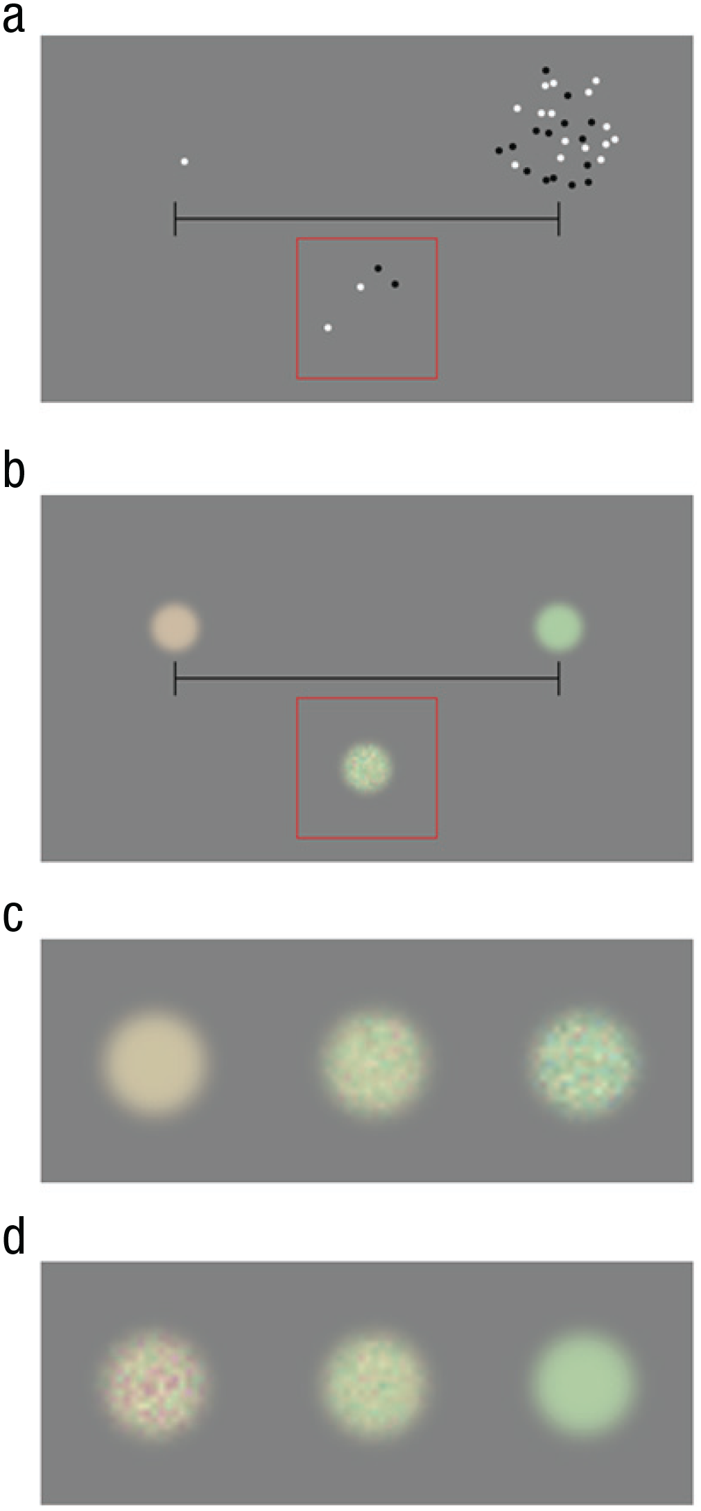
Experimental paradigm and stimulus examples. In the number-line task (a), participants indicated the number of dots in a stimulus (the cloud of dots inside the red box) by touching the appropriate location on a number line. In the color-line task (b), participants indicated the color of a stimulus patch (inside the red box) by touching the appropriate location on a color line. Example stimuli for the first color-line task are shown in (c). Chromatic noise was added progressively from left (peach) to right (citron), interpolating linearly between the two extremes. Example stimuli for the second color-line task are shown in (d). Chromatic noise was added progressively from right (citron) to left (peach), again interpolating linearly.

For the number-line experiment, the instructions were as follows:

This is a number line with one element on the left extreme and 30 items on the right. When you touch the screen, a cloud of dots will appear within the box below the line, and your task is to indicate where the number of dots would fall on the number line. The other stimuli will follow suit.

For the color-line experiment, the instructions were as follows:

This is a color line with one colored disk on the left and one on the right. When you touch the screen, a colored disk will appear within the box below the line, and your task is to indicate where the color of the disk would fall on the color line. The other stimuli will follow suit.

At this stage, the participant would start the experiment by tapping on the screen border. After 2 s, the first to-be-mapped stimulus appeared (lasting 1 s). Trials following the first were automatically presented by the program after each response (1-s interstimulus interval). Using a finger on their dominant hand, participants touched the location on a number line that they estimated would correspond with the number of dots in the stimulus (number-line experiment) or the location between two anchor colors on a “color line” that they estimated would correspond to the color of the stimulus. The touch triggered a sound signaling that the response was saved. There was no time pressure, and no feedback was given about accuracy. Participants were tested in a quiet room in a single session consisting of nine trials (lasting less than 2 min).

The order of stimuli was determined by a balanced Latin square such that each stimulus set (cloud of dots or color patch) was uniformly sampled across participants. For the number-line task, each dot cloud was tested by at least eight participants, each of whom saw that cloud on at least one trial. For each of the two color-line tasks, each stimulus was tested by five participants, each of whom saw that color patch on at least one trial.

Stimuli

The number line was 14-cm long, and there was one dot on the extreme left and a 30-dot cloud on the extreme right (see Fig. 2). The stimulus to be mapped appeared 7 cm below the line within a 5.5-cm × 5.5-cm square frame. Stimuli were clouds of nonoverlapping 0.2-cm-diameter dots, half of which were white and half black, displayed at 90% contrast on a gray background (luminance = 104 cd/m²). Dots were constrained to fall inside a virtual circle of 5 cm in diameter. Each participant was tested with nine unique stimulus sets, listed in Table 1.

Table 1.

Stimulus Parameters for the Number-Line and Color-Line Experiments

Stimulus	Number line	Color line		Reverse color line
	Number of dots	Hue	σhue	Hue	σhue
1	4	0.12667	0 a	0.12667	0.08667
2	7	0.14667	0.02333	0.14667	0.07667
3	10	0.16667	0.03333	0.16667	0.06667
4	13	0.18667	0.04333	0.18667	0.05667
5	16	0.20667	0.05333	0.20667	0.04667
6	19	0.22667	0.06333	0.22667	0.03667
7	22	0.24667	0.07333	0.24667	0.02667
8	25	0.26667	0.08333	0.26667	0.01667
9	28	0.28667	0.09333	0.28667	0 a

a

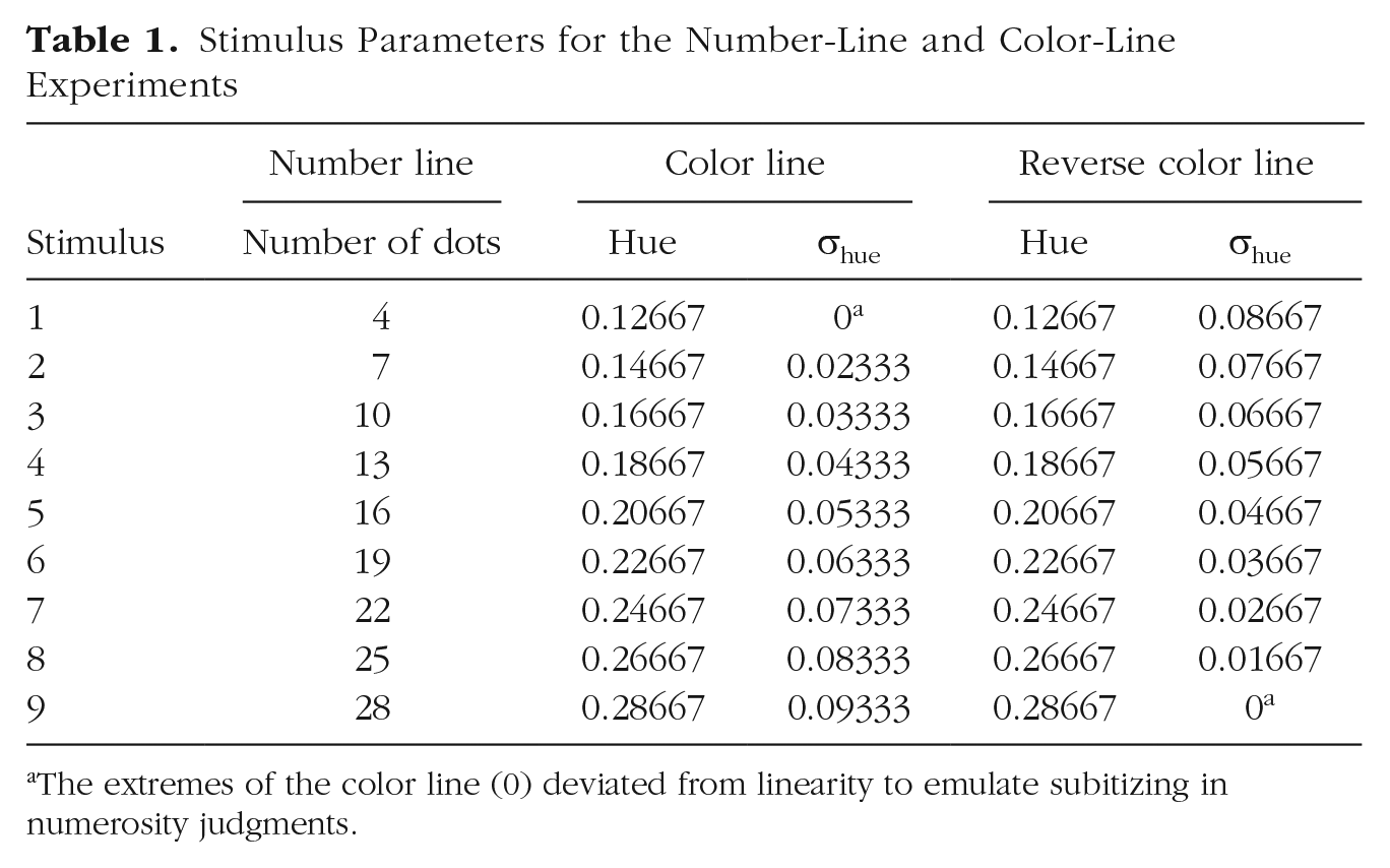
The extremes of the color line (0) deviated from linearity to emulate subitizing in numerosity judgments.

The color line was analogous to the number line, except that the stimuli were colored circles 1.4 cm in diameter rather than dot clouds (see Fig. 2). The color line was delimited by two reference color patches: peach-orange on the left and bright citron-green on the right. We defined the colors from the hue, saturation, value (HSV) color space: peach = 0.1, 0.2, 0.8; citron = 0.3, 0.2, 0.8. These values yielded stimuli with the following Commission Internationale de l’Éclairage (CIE) color-space coordinates—peach: x = 0.346, y = 0.359 (luminance = 140 cd/m²); citron x = 0.316, y = 0.382 (luminance = 143 cd/m²), measured on screen by a CS-100 Minolta photometer. The base hues of the patches were linearly interpolated between these two extremes with MATLAB’s implementation of HSV color space to produce nine unique stimuli (see hues in Table 1), corresponding to the same positions on the line as the number stimuli (see Column 2 in Table 1).

To emulate the noise gradient that presumably drives the increase in response variance with increases in numerosity, we perturbed the hues with pixelated Gaussian noise. We created small (21 × 21 pixels) images, defining the hue of each pixel by randomly drawing from a Gaussian distribution centered at the base hue with variable standard deviation ( ${\sigma }_{\mathrm{hue}}$ ). The images were then upscaled by bicubic interpolation to produce images of 210 × 210 pixels (effectively, low-pass-filtered noise patterns with a cutoff of 5 cycles per degree) and multiplied by a two-dimensional circular vignette of 1.4 cm diameter having a sigmoidal roll-off of 0.4 cm (14%–86% opacity).

In the first condition, the noise amplitude increased almost linearly from peach to citron: ${\sigma }_{\mathrm{hue}}$ = 0 for peach patches to ${\sigma }_{\mathrm{hue}}$ = 0.1 for citron patches (see Table 1 for precise values). In the second condition, we applied the reverse gradient (noise highest for colors on the left, decreasing linearly toward the right; see Table 1). Saturation (S in the HSV color space) of the stimuli was unaffected by noise, but we included a small luminance noise to mask possible luminance cues that could interfere with hue judgments by adding Gaussian noise to the V coordinate of the HSV color space with ${\sigma }_{\mathrm{value}}$  of 0.05.

Analysis and curve fitting

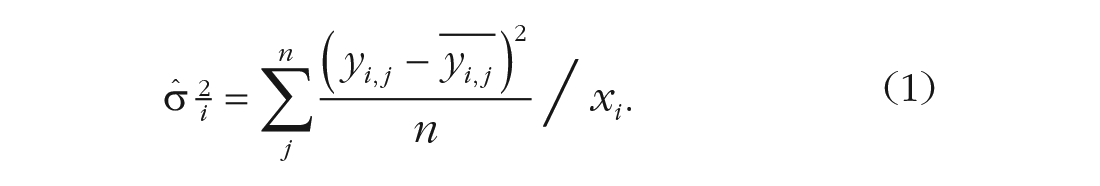
We first combined data from individual participants to create an aggregate observer for every condition and trial number, from which we calculated the dispersion index. We first computed, for each numerosity $i$ , the variance of the raw responses $y_{i,j}$ (where $i$ is the numerosity condition and $j$ the counter running through the aggregate observer at that numerosity and trial number), normalized by the stimulus numerosity $x_i$ :

$$\hat{\sigma }\frac{2}{i}={\displaystyle \sum }_j^n\frac{{\left(y_{i,j}-\overline{y_{i,j}}\right)}^2}{n}/x_i.$$

(1)

We then averaged these normalized variances across the nine numerosity stimuli and took their square root to obtain the dispersion index:

$$\mathrm{Dispersion}\mathrm{index}=\sqrt{{\Sigma }_i^9{\hat{\sigma }}_i^2/9}.$$

(2)

For the color-line experiments, and as an alternative analysis to the numerosity data (see Fig. S1 in the Supplemental Material available online), we quantified response scatter with Weber fractions, the normalized standard deviations for each numerosity $i$ :

$${\mathrm{Weber}\mathrm{fraction}}_i=\sqrt{{\displaystyle \sum }_j^n\frac{{\left(y_{i,j}-\overline{y_{i,j}}\right)}^2}{n}}/x_i.$$

(3)

Then we averaged across all numerosities tested at a given trial.

For the number-line and first color-line tasks, we fitted average responses with a log-linear model that was created from an additive mixture of a linear and logarithmic function, as used by Anobile, Cicchini, and Burr (2012):

$$y=a\left(\left(1-\lambda \right)x+\lambda .K.{\log }_{10}\left(x\right)\right).$$

(4)

Each fitting curve was determined by two parameters: $\lambda$ , the relative contribution of the logarithmic and linear components, and $a$ , a scaling factor that determines the overall height of the fit. $K$ is a constant set to $X_{\max }/{\log }_{10}\left(X_{\max }\right)$ to balance the relative contributions of the linear and log components.

For the reverse color line, we fitted the growth function with a reverse log-linear equation, which was the mirror symmetrical version of Equation 4, given by flipping both $x$ and $y$ . The function is anchored at the upper end (right) of the response line and free to vary at the lower end (left):

$$y=-a\left(\left(1-\lambda \right)(30-x)+\lambda .K.{\log }_{10}\left(30-x\right)\right)+30.$$

(5)

Bayesian modeling

We modeled the behavior of an ideal observer who combines optimally prior knowledge with current sensory evidence. In such a model, estimates are the combination of the current observation (centered on the stimulus $x$ ) and prior knowledge (in this case, the center of the response space $X_{\max }/2$ ):

$$y=x\left(1-w_p\right)+w_p.X_{max}/2.$$

(6)

For an optimal observer, the weight of the prior $w_p$ is proportional to the relative reliabilities $({\sigma }^{-2})$ of the two sources of information, likelihood and prior:

$$w_p=\frac{{\sigma }_P^{-2}}{{\sigma }_P^{-2}+{\sigma }_L^{-2}}=\frac{{\sigma }_L^2}{{\sigma }_L^2+{\sigma }_P^2}.$$

(7)

For any given ${\sigma }_P$ , the behavior of the model varies with sensory variance ${\sigma }_L^2$ for each numerosity. For low variance ( ${\sigma }_L^2)$ , the weight of the prior approaches zero, so the main contribution to the response will come from the current observations, leading to a near linear (and veridical) response curve (gray curve in Fig. 1b). For high variance, however, the prior becomes important, leading to clear compressive nonlinearities (green curve in Fig. 1b). If variance scales with stimulus intensity x (e.g., shot noise), the relative contribution of the current observation and prior will vary across the stimulus range: For small values of x, variance is low, leading to little weighting of the prior, whereas for large values of x, variance increases, leading to higher weighting of the prior and a departure from linearity toward the mean.

In our fitting approach, response variance was determined experimentally; the only free parameter for the fit was ${\sigma }_P$ , the width of the prior. We assumed that this did not change over time and simultaneously fitted the nine trials with the same value of ${\sigma }_P$ .

Results

Number-line experiment

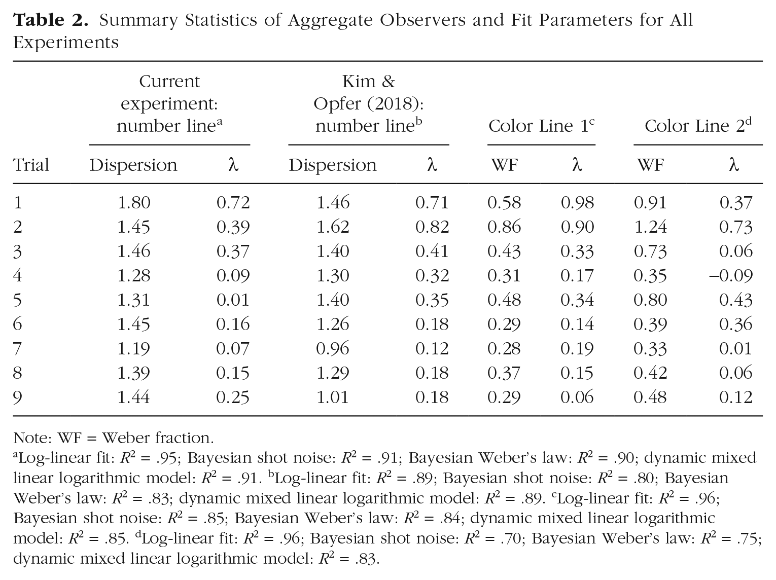
We first replicated Kim and Opfer’s (2018) study, asking 78 students to make nine consecutive judgments about the number of dots in a stimulus set and to indicate those judgments on a number line (see Fig. 2). The results of the first, fifth, and ninth judgments for Kim and Opfer’s and our data sets are shown in Figure 3. The trend was very similar. The first judgments (see Figs. 3a and 3d) showed the greatest nonlinearity, and then the mapping became progressively more linear. The orange curves show the best log-linear fit to the data (Equation 4; also see Table 2 for values of $\lambda$ ). In both studies, the logarithmic component $\lambda$ decreased steadily over trials, from 0.71 on Trial 1 to 0.17 on Trial 9 in our data and from 0.72 to 0.25 in Kim and Opfer’s data (see Table 1 and ordinates of Figs. 3h and 3i).

Fig. 3.

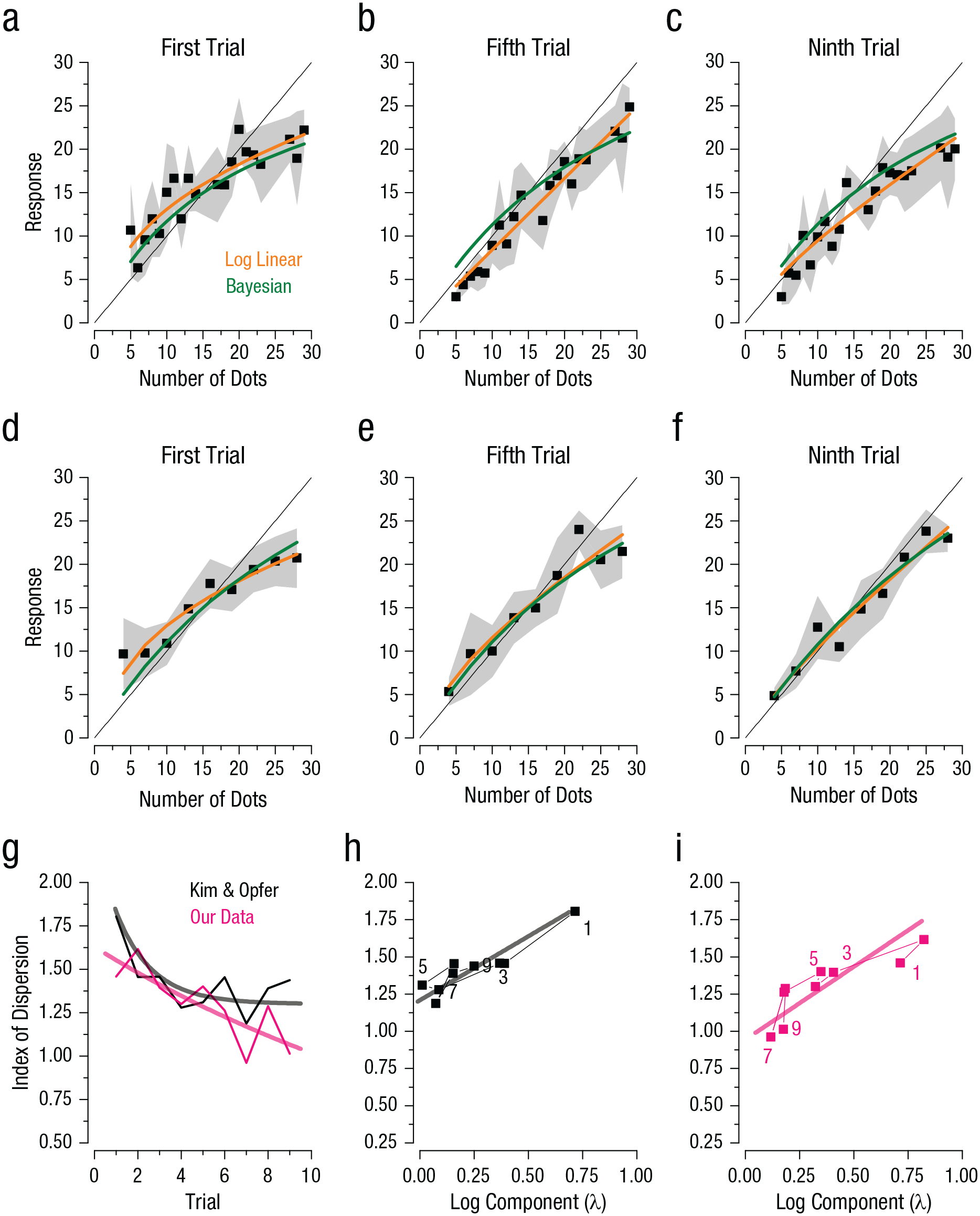
Results from the number-line experiment. The top row shows the average response from the data set of Kim and Opfer (2018) on the (a) first, (b) fifth, and (c) ninth trials as a function of the number of dots in the stimulus. The middle row shows the average response from the current data set on the (d) first, (e) fifth, and (f) ninth trials as a function of number of dots in the stimulus. Squares indicate responses, and the shaded regions indicate 95% confidence intervals. Fits of the log-linear model (Equation 4) are shown in orange, and predictions of the Bayesian observer based on a measured index of dispersion are shown in green. Indices of dispersion (g) are shown as a function of trial number, separately for Kim and Opfer’s data set and our data set. Continuous curves are fits of an exponential decay function, $ln(y)=A-kx.$ In (h) and (i), the correlation between response curvatures (as indexed by the log component of Equation 4) and indices of dispersion across trials is shown for Kim and Opfer’s data set and our data set, respectively. In (h) and (i), thick lines indicate best-fitting linear regressions, and numerical values indicate trial numbers.

Table 2.

Summary Statistics of Aggregate Observers and Fit Parameters for All Experiments

Trial	Current experiment: number line a		Kim & Opfer (2018): number line b		Color Line 1 c		Color Line 2 d
	Dispersion	λ	Dispersion	λ	WF	λ	WF	λ
1	1.80	0.72	1.46	0.71	0.58	0.98	0.91	0.37
2	1.45	0.39	1.62	0.82	0.86	0.90	1.24	0.73
3	1.46	0.37	1.40	0.41	0.43	0.33	0.73	0.06
4	1.28	0.09	1.30	0.32	0.31	0.17	0.35	−0.09
5	1.31	0.01	1.40	0.35	0.48	0.34	0.80	0.43
6	1.45	0.16	1.26	0.18	0.29	0.14	0.39	0.36
7	1.19	0.07	0.96	0.12	0.28	0.19	0.33	0.01
8	1.39	0.15	1.29	0.18	0.37	0.15	0.42	0.06
9	1.44	0.25	1.01	0.18	0.29	0.06	0.48	0.12

Note: WF = Weber fraction.

a

Log-linear fit: R² = .95; Bayesian shot noise: R² = .91; Bayesian Weber’s law: R² = .90; dynamic mixed linear logarithmic model: R² = .91. ^bLog-linear fit: R² = .89; Bayesian shot noise: R² = .80; Bayesian Weber’s law: R² = .83; dynamic mixed linear logarithmic model: R² = .89. ^cLog-linear fit: R² = .96; Bayesian shot noise: R² = .85; Bayesian Weber’s law: R² = .84; dynamic mixed linear logarithmic model: R² = .85. ^dLog-linear fit: R² = .96; Bayesian shot noise: R² = .70; Bayesian Weber’s law: R² = .75; dynamic mixed linear logarithmic model: R² = .83.

The two strong predictions of the Bayesian model are that response precision should be poorest on the first trial and then progressively improve and that the imprecision should correlate positively with the magnitude of nonlinearity. We estimated response precision as the square root of the average dispersion index of the responses, defined as the variance at each numerosity normalized by the numerosity (see Method for details and Discussion for rationale). Figure 3g plots this precision index (higher numbers imply greater imprecision) as a function of trial number for the two experiments. In both cases, the index was high in the first trial and then steadily decreased over time, following an exponential decay (exponential fit: R² = .49, p < .001 and R² = .53, p < .001 for Kim and Opfer’s data set and our data set, respectively). Figures 3h and 3i plot the dispersion index against the logarithmic factor $\lambda$ —the index of nonlinearity—for each of the nine estimates, separately for the two experiments. The two measures were strongly correlated and highly significant (r = .92, p < .001 for Kim and Opfer’s data set; r = .85, p = .002 for our data set; ps one tailed).

The poor precision observed on the first trial predicts that the prior will have a relatively greater effect, leading to the nonlinearity. This qualitative relationship is clear in Figures 3h and 3i, but can the increase quantitatively predict the nonlinearity? The green curves in Figures 3a to 3f show the Bayesian predictions, obtained by combining the prior with the data (likelihoods in the Bayesian model) and weighting the contribution of the prior by the relative reliabilities (inverse variances). To smooth the variance estimates, we assumed that response variance increased linearly with numerosity (Equation 1), leading to a constant index of dispersion (Equation 2). The only parameter free to vary was the width of the prior, assumed to be positioned in the center of the number line and to remain constant for all trials (one free parameter for nine fits). It is clear that this Bayesian model captured the data well, showing the same compressive nonlinearity as the logarithmic fits. The fits are also quantitatively good: Average R² was .80 and .91, respectively, for Kim and Opfer’s data and our data, compared with .90 and .94, respectively, for the log-linear fit (see Table 2). Considering that the nine log-linear fits were independent, each with two free parameters, whereas the Bayesian fit had only one parameter for all nine fits, the Bayesian fits are respectable, even if not quite as good. More importantly, the green curves were derived from an efficiency-based model rather than merely fitting the data. To replicate other models in the literature, we also ran Kim and Opfer’s dynamic mixed linear logarithmic model, in which the mixture of linear and log components is updated from trial to trial, depending on the stimulus presented. This model has fewer parameters than the nine independent fits and yielded fits with an average R² of .90 and .91 for the two data sets (see Table 2).

In these fits, we assumed that variance was directly related to numerosity, as has been reported, consistent with variability determined by shot noise or Poisson noise, typical for distributions of discrete events, such as photons (Schottky, 1918). However, it is important to stress that this assumption was not essential for the model. Other assumptions, including Weber’s law (constant coefficient of variability), led to similarly good predictions, as we show in Figure S1 and Table 2.

Color-line experiments

The previous sections showed strong correlational evidence for the Bayesian model: Precision was poorest on the first trial and then steadily improved. The precision indices were good predictors of the results of all nine trials without additional free parameters. However, although the correlational evidence was strong, the strongest stress test for any theory is whether an experimental manipulation can cause a predicted outcome. Because almost all psychophysical judgments are subject to regression to the mean (Hollingworth, 1910), it should in theory be possible to obtain compressive logarithmic-like mapping with other nonnumerical judgments, such as color-to-space mapping. All that is needed for response compression, besides the mean acting as a prior, is a gradient of thresholds, so one end of the mapped attribute is more susceptible to the prior and therefore more attracted to the mean.

To test this possibility, we designed a task in which observers mapped a colored patch onto a color line, which varied smoothly from peach-orange at left to citron-green at right (see Fig. 2c). The color patches were perturbed by chromatic noise, which increased progressively from no noise for peach patches to maximum noise for citron patches (for details, see the Method section). The idea of this manipulation was to progressively increase thresholds, with a Weber-like dependence on stimulus magnitude simulating the presumed internal noise underlying numerosity judgments (which increases monotonically with numerosity). This in turn should cause more Bayesian regression to the mean for mappings on the right end of the color line, thereby creating a compressive, logarithmic-like nonlinearity.

The results are shown in Figures 4a to 4c. The mapping followed the same pattern as the number-line mapping. The first trial had a very strong logarithmic component ( $\lambda$ = 0.98), which gradually decreased over the next nine trials (down to $\lambda$ = 0.06 at the ninth trial). As we observed in the previous experiments, response variability was also highest on the first trial and then decreased exponentially (R² = .39, p = .001; see Fig. 4g). Again, the variability (indexed as a Weber fraction) correlated significantly with the logarithmic component (r = .87, p < .001, one tailed; see Fig. 4h). Furthermore, these indices directly predicted the compressive nonlinearity: With only one degree of freedom for all nine fits (the width of the prior), the theory-based model explained 85% of the variance, compared with 87% explained by the descriptive log-linear fit, which had 18 free parameters and was not theoretically motivated (see Table 2).

Fig. 4.

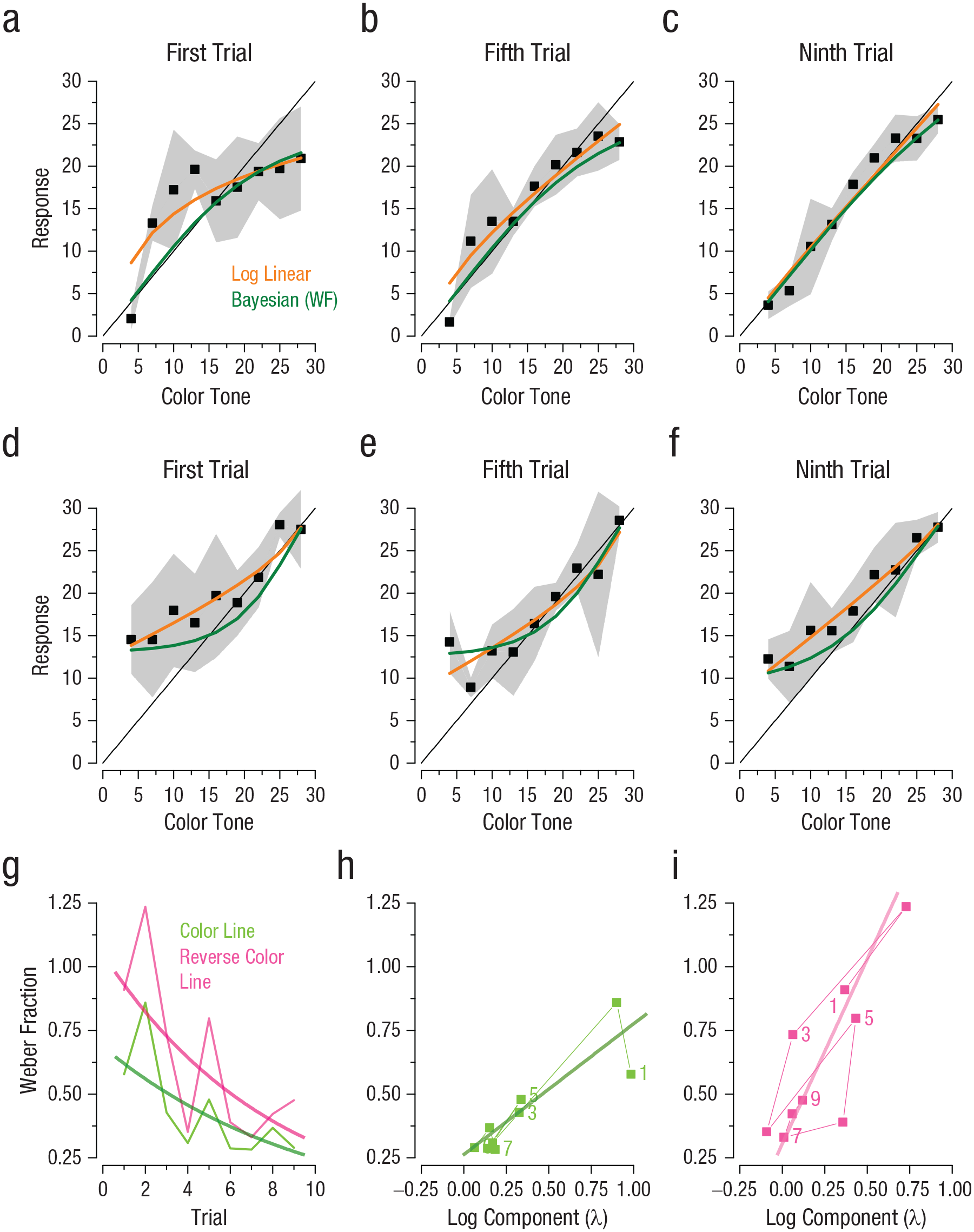
Results from the color-line experiment. The top row shows the average response from the data set of Kim and Opfer (2018) on the (a) first, (b) fifth, and (c) ninth trials as a function of color tone (hue). The middle row shows the average response from the current data set on the (d) first, (e) fifth, and (f) ninth trials as a function of color tone. Squares indicate responses, and the shaded regions indicate 95% confidence intervals. Stimuli ranged from peach to citron, in 30 equal steps. Fits of the log-linear equation (Equation 5) are displayed in orange. Predictions of the Bayesian observer are in green. Progression of Weber fractions (WFs) is shown (g) as a function of trial number for the two color-line tasks. Continuous curves are fits of an exponential decay function, ln(y) = A − kx. In (h) and (i), the correlation between λ and dispersion index across trials is shown separately for the first and second color-line tasks, respectively. The thick lines indicate best-fitting linear regressions, and numerical values indicate trial numbers.

Although it has been suggested that number coding may follow a logarithmic law, no such suggestion has ever been applied to color, usually described as being fairly linear around the circle (Wyszecki & Stiles, 1982). It therefore seems unlikely that the compression reflects an intrinsic static nonlinearity in color coding but is a consequence of the asymmetric added noise. To test this hypothesis further, we repeated the experiment with an inverted noise gradient, maximal at the peach end and decreasing progressively to citron (see Fig. 2d). Under these conditions, the nonlinearity in the mapping became expansive rather than compressive. We fitted the data with a flipped log-linear function anchored at the high end (Equation 5), where the nonlinear component was captured by the log component (λ) and was free to vary. As is obvious by the fits (orange curves), there was a strong accelerating component in the first trials, which gradually decreased over trials. Again, the increase in reliability over trials was well described by exponential decay of Weber fractions (R² = .16, p = .007; see Fig. 4g), and dispersion at each trial correlated significantly with the nonlinear, logarithmic component of the fit (r = .87, p = .001, one tailed; see Fig. 4i). The green curves in Figures 4d to 4f show the parameter-free Bayesian model, which fitted the data well, explaining 70% of the variance (with nine inverted log-linear fits explaining 86%).

First-trial responses on number-line task across experiments

An important prediction of our approach is that nonlinear response patterns arise whenever either the participant or the condition is accompanied by a high noise level, whereas more linear patterns emerge when observers are precise and conditions not so taxing.

To address these predictions, we examined two data sets provided by Kim and Opfer (2018), which are the only ones available that employed a balanced Latin square design. One is their Study 4, which examined number-line mapping of nonsymbolic numbers in young children. As already reported in the literature, a strong nonlinearity emerges at a young age (5–6 years). These data were previously fitted with the log-linear model, which became saturated at λ of 1. To better quantify the fit, we relaxed the boundary conditions of the log-linear fit and reported a logarithmic component λ equal to 1.85. Indeed, the curve was nearly flat (R² for the logarithmic fit was only .14), implying that it predicts the data little better than the mean (see Fig. 5a). Nevertheless, if our model is correct, the stronger nonlinearity in children should be explained by high response variability in children. The root index of dispersion for the children’s aggregate data on the first trial was 2.23 (see blue square in Fig. 5d), compared with 1.80 for the adults in their study.

Fig. 5.

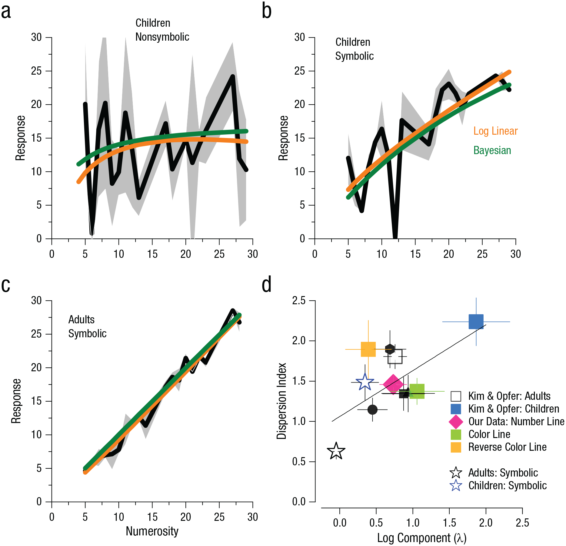
Responses on the first trial of the number-line task across data sets and dispersion index across experiments. Responses from Kim and Opfer’s (2018) Study 4 are shown for (a) 5- to 6-year-old children’s mapping of nonsymbolic numerosities (number of dots in dot clouds) to a number line, (b) children’s mapping of symbolic numerosities (numerals) to a number line, and (c) adults’ mapping of symbolic numerosities (numerals) to a number line. Fits of the log-linear model (Equation 4) are shown in orange, and predictions of the Bayesian observer based on a measured index of dispersion are shown in green. Shaded regions indicate 95% confidence intervals. Dispersion indices of children and adults across all studies and tasks (d) are plotted against log component $\lambda$ of log-linear fit. Black symbols show results from Kim and Opfer’s studies on adults (square, triangle, circle, and hexagon refer to Studies 1–4, respectively). Error bars indicate standard errors. The diagonal line shows the correlation across all studies (excluding the aggregate data set of Kim and Opfer).

The other data set is also from Study 4 by Kim and Opfer (2018), in which the numerosity to be mapped was presented as Arabic numbers (see Figs. 5b and 5c). In this case, even the first trial displayed very little logarithmic compression (0.34 for the children group and −0.05 for the adult group; see blue and black stars, respectively, in Fig. 5d). In line with our hypothesis, this was also accompanied by a reduction of the root index of dispersion of 1.48 and 0.64, respectively, for the two groups.

The relationship between the curvature of responses (as indexed by λ) and sensory resolution was a general characteristic of the data. Figure 5d shows the data for the various experiments by Kim and Opfer (2018), together with that of our studies. Clearly, the conditions with the highest dispersion indices also had the highest logarithmic compression (r = .66, p = .018).

Discussion

We tested the notion that the compressive nonlinearities in number-to-space mapping result from efficient Bayesian strategies rather than from innate logarithmic coding. We first replicated the study by Kim and Opfer (2018), finding that there were strong compressive nonlinearities on the first trials of each participant but that the data became progressively more linear over trials. As predicted, response precision was poorest on the first trials and then steadily improved, paralleling the linearization of responses. The magnitude of the precision indices quantitatively predicted the nonlinearities of both our and Kim and Opfer’s results, with only one degree of freedom for the nine fits (the prior width). We also predicted and observed lower precision indices in children’s data and higher precision for symbolic numbers. Interestingly, our conclusions fit both our own data, collected from college students in Italy, and those of Kim and Opfer, collected from adults and young children in the United States, equally well. This gives confidence that the phenomena under study are a general trait of human behavior and may generalize beyond the present research.

Kim and Opfer (2018) explained the progressive linearization of responses across trials, assuming a specific trial-by-trial update of the mapping prompted by how similar the previous and current stimuli were to the end point, within their dynamic mixed linear logarithmic model. Goodness of fits with this model (which has more parameters and includes a scaling factor) were similar to those of the Bayesian fits. However, our model provides a much simpler explanation, suggesting that linearization occurs because of the spontaneous improvement of precision with training. However, how the central and sequential priors combine is still an open question for further studies.

The strongest evidence for Bayesian contextual effects rather than logarithmic encoding in number-line mapping was the color-line mapping experiments. Color representation is best conceived as circular (Shevell, 2003), but a portion of this space can be represented as a line to which participants can reliably map specific colors. When color noise was added to the samples to be mapped, participants mapped color to space in a logarithmic fashion. However, for noise increasing in the opposite direction, the mapping became exponential. It is clearly unreasonable to suggest that color hues are encoded logarithmically, in any particular direction, but even more so that the encoding could shift from logarithmic to exponential when noise is selectively added. Efficient Bayesian contextual processes provide a far more parsimonious explanation for both color-line and number-line mapping. One difference between the number-line and color-line experiments is that for numerosity, the noise driving the decrease in precision with numerosity was internal, whereas for the color-line experiments, the noise was external and visible, and internal noise was invisible. But despite this difference, the external, visible noise created compressive nonlinearity, as did internal noise on numerosity estimation: Both forms of noise increased response variance to cause the compressive nonlinearity, as predicted both qualitatively and quantitatively.

When reliability (inverse variance) is low, other signals such as a central prior become relatively important, causing the well-known regression to the mean (Hollingworth, 1910). If the nonlinear color mapping results from efficient Bayesian processes, there is little need to invent arbitrary mechanisms such as logarithmic coding for number processing. When participants are most uncertain, such as on their first trial (when they have the least experience in the task), they weight their judgments heavily with prior information, including the mean position they are mapping to.

Most previous literature has assumed that the central tendency prior is derived from statistical regularities of the environment (Adams et al., 2004; Cicchini et al., 2012; Jazayeri & Shadlen, 2010) during an experimental session or from daily experience. These are very rapid processes that can recalibrate responses in as little as three trials (Berniker et al., 2010) but cannot explain context effects on the very first trial. However, our results show that they can and do exist, at least in experiments such as number-line and color-line mapping, in which the response space is on continuous display. The system is clearly flexible and efficient, incorporating information from all possible sources. Our results suggest that in the absence of statistics of the perceptual past, participants derive a prior from the response space itself, which, on average, will correspond to the center of the space. In this respect, our model is surprisingly successful because the prior for the first trial is not a free parameter but is assumed to be central.

The notion that perceptual systems logarithmically encode physical qualities goes back 160 years, to the founder of the field of psychophysics, Gustav Fechner (1860). The idea neatly explained many common psychophysical phenomena, including the Weber-Fechner law (whose integral is logarithmic). This simple and compelling idea dominated psychophysics textbooks for a century before being challenged by Stevens (1957), who showed that observer estimates of stimulus intensity did not typically follow a logarithmic function but rather a power function, seriously questioning logarithmic encoding as a general law. More recent research explains nonlinearities in sensory transduction as the action of dynamic gain control and normalization mechanisms (Carandini & Heeger, 2011; Shapley & Enroth-Cugell, 1984), which optimize systems to prevailing levels of luminance, contrast, and so on and predict compressive nonlinearities in most sensory mechanisms.

Many modern approaches to number cognition treat it as a perceptual system, variously termed “the number sense” (Dehaene, 2011) or a “primary visual property” (Burr & Ross, 2008, p. 425). As with all other perceptual systems, number systems adapt dynamically to the prevailing level of numerosity (Burr & Ross, 2008), a clear signature of the gain-control processes that explain the Weber-like behavior of discrimination thresholds (Carandini & Heeger, 2011). It is therefore highly probable that numerosity is encoded like other dynamically adaptable perceptual systems, rather than performing static logarithmic transformations. Indeed, as Gallistel and Gelman (1992) have pointed out, logarithmic encoding would be problematic for many reasons, including the fact that it would hinder addition, fundamental for dealing with numbers.

Early support for logarithmic encoding of numbers was that numerosity discrimination shows scalar variability, the tendency to follow the Weber-Fechner law (Dehaene, 2003; Ross, 2003; Whalen et al., 1999), and that the bandwidths of numerosity-tuned neurones scale with numerosity (Nieder, 2016). However, Weber’s law is not always observed: At low “subitizing” numerosities, the increase is steeper than predicted by Weber’s law (Dehaene, 2003), and at high numerosities, the increase is shallower, closer to the square root (Anobile et al., 2014). In number-line tasks, precision follows a square root rather than Weber’s law (Cicchini et al., 2014; Pomè et al., 2021). A square-root law is the signature of shot noise or Poisson noise, the intrinsic noisiness of the stimulus, of which photon noise is a clear example (Schottky, 1918). The square-root law is common in psychophysics, including the de Vries-Rose law in luminance discrimination (Rose, 1948), usually taken as a signature that discrimination is limited by the noisiness of the stimulus rather than by special encoding mechanisms. Similarly, in our model, shot noise is determined by the stimulus rather than an encoding strategy. However, the square-root law is not essential for the model: Figure S1 shows that scalar variability (Weber’s law) will also produce the same result, as will any positive dependence on numerosity.

We conclude that the compression of the number line results from efficient Bayesian-like processes that take advantage of prior information to reduce error. Although number-to-space mapping can be well fitted by log-linear functions, this does not in itself prove the existence of intrinsic logarithmic encoding mechanisms for numerosity. The compressive nonlinearity more likely reflects mechanisms evolved to exploit contextual effects to maximize perceptual efficiency. However, it is important to emphasize that this study does not minimize the usefulness of the number line as a diagnostic test for numerical understanding. Indeed, our results show that Bayesian processes account for the higher nonlinearities in mapping in children. Whatever the mechanisms behind the nonlinearity, the number-line task remains an informative diagnostic tool (Anobile et al., 2019; Berteletti et al., 2010; Geary et al., 2008). However, what our research shows is that it is also vital to elucidate the mechanisms that lead to deviations from perfectly linear behavior to better interpret the results of this simple and widespread test of basic numerical skills.

Supplemental Material

sj-docx-1-pss-10.1177_09567976211034501 – Supplemental material for Uncertainty and Prior Assumptions, Rather Than Innate Logarithmic Encoding, Explain Nonlinear Number-to-Space Mapping

Supplemental material, sj-docx-1-pss-10.1177_09567976211034501 for Uncertainty and Prior Assumptions, Rather Than Innate Logarithmic Encoding, Explain Nonlinear Number-to-Space Mapping by Guido Marco Cicchini, Giovanni Anobile, Eleonora Chelli, Roberto Arrighi and David C. Burr in Psychological Science