
Abstract
The measure for assessing the acoustic quality of the rail surfaces, the acoustic roughness, is defined in the EN 15610 standard. It is shown that this standard contains gaps with regard to the applied procedures for processing the raw data to the quantity of acoustic roughness. Additions to the standard appear necessary to ensure better comparability of the results. A piece of rail tactilely measured by METAS (Swiss Federal Institute of Metrology) was used as a reference. Measurement data recorded by a laser triangulation sensor was used to quantify the adjustments to the standard. This paper provides an overview of the individual processing steps and systematically examines possible additions to the standard to improve the quality of the outcome. Special emphasis was given to a method for outlier removal, pre-filtering, spike removal, curvature correction and calculation of one-third octave bands. It becomes apparent that different implementations can have a significant impact on the final result. The filter used, the wavelength ranges, the methodology for removing outliers should be specified. The spike removal, curvature correction and the calculation of the one-third octave bands should be supplemented in detail to reduce ambiguities in the implementation.
Keywords
Introduction
Traffic noise can cause various health problems as described by Héritier et al.
1
and Dratva et al.
2
It is therefore an endeavour to reduce the noise from rail traffic as much as possible. A large part of railway noise originates from the rolling noise of the vehicle, respectively, from the wheel-rail contact as described by Thompson.
3
According to Szwarc et al.,
4
this is especially true for the speed range between
There are numerous standards dedicated to the topic of noise emission and measurement in the railway sector. EN ISO 3381 12 deals with the topic of noise measurement in rail vehicles. EN ISO 3095, 13 on the other hand, deals with noise measurement on vehicles in general. EN 15610 14 focuses on the noise development resulting from the wheel-rail contact and the roughness of the respective components in contact. The procedure for calculating the acoustic roughness is given by EN 15610. 14 Despite this definition, ambiguities remain in the data processing which can influence the result.
The aim of this paper is to develop an optical acoustic roughness measurement set-up, which can operate on the moving train. The direct measurement of the longitudinal profile of the rail is carried out using laser triangulation sensors. In the following, the further processing of the measured data to the acoustic roughness will be systematically examined and suggestions for supplementing its definition will be recorded. The target of this paper is to present a calculation of acoustic roughness to give a more stable definition of the evaluation process.
Method
Experimental setup
A test setup equipped with a reference rail was used. The reference rail has a ground profile, which had been tactilely measured with a measuring tip size of Experimental setup with the installed laser triangulation sensors indicated by numbers 1–4.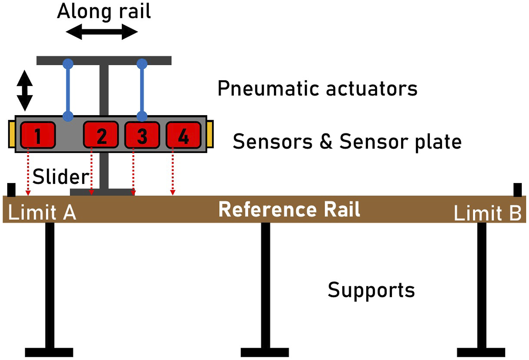
The sensor plate carrying the sensors is connected to the slider with pneumatic actuators for an additional test series involving the simulation of the train suspension. The setup is fixed such that the pneumatic actuators are not actuated during the measurement. Thus, the degree of freedom perpendicular to the rail is suppressed. Tests were performed with a clean rail as well as with a rail contaminated with dust or water. The purpose of the latter was to create a disturbed data with real interferences that exist on the rail network set in order to challenge the optical measurement and the data processing. The raw data was stored and further processed to the acoustic roughness in a separate step. Only the data of sensor one was used for the investigations. The combination of all sensor values and the possible improvement of a measurement result are part of a follow-up study.
Data processing
The following processing steps were followed: (1) Import of the TDMS (Technical Data Management Streaming) data: The analog data was recorded with a cRIO 9045 from National Instruments. The TDMS file format of National Instruments was used due to its integrability into the LabView software and the resulting small file size. The data must also be converted from analog voltage signals to distance values. (2) Outlier removal: As the measurement was carried out optically, unfavourable reflections (e.g. speckle) can become noticeable in the form of outliers in the data set. The same applies to dust or water being present on the rail. Both were artificially applied to the rail in experiments. Outliers influence the measurement result and require further steps of the data post-processing. Therefore, the IQR (interquartile range) method for outlier removal was investigated and implemented. The objective is to remove the outliers without distorting the significance of the original data set. Usually outliers differ significantly from the rest of the data set. Thus, the outlier removal must not be set too sensitively; otherwise it will also remove spikes in the same way as the spike removal procedure. (3) Resampling: Since the measurements were not carried out at a uniform speed, the data point distances in the longitudinal direction are not constant in the unprocessed form. Therefore, linear interpolation was used to generate a constant data point spacing at the points of the reference data set. For the provided reference data in this setup, this leads to a sample spacing of (4) Pre-Filter of Raw Data: The wavelength range results from the range of interest given in the standards, which focusses on the corresponding train speeds where rail corrugation is deemed relevant for noise emission. EN 15610
14
specifies a range between (5) Profile comparison: Before further processing the measurement data for the acoustic roughness, a profile comparison to the METAS measurement can be performed. The longitudinal profile measured by METAS was compared with the profile estimates from the optical measurement in the time domain. The longitudinal offset of the measurements from each other were corrected. The following values were calculated and compared: a. Root-mean-square deviation b. Correlation coefficient c. Mean value of the absolute error d. Integrated absolute error e. Mean value of the relative error (6) Spike removal: According to EN 15610
14
spikes in the measurement data that are too large must be removed (e.g. small impurities) for the determination of the acoustic roughness. They could have a negative influence on the result in the short-wave range. The spike removal process is defined for a tactile measuring method with a probe tip radius of Spike removal procedure.
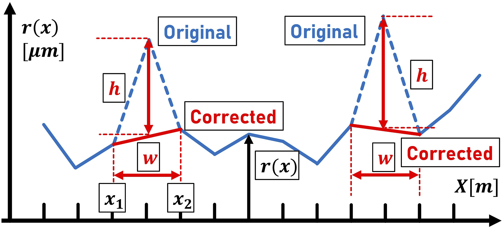
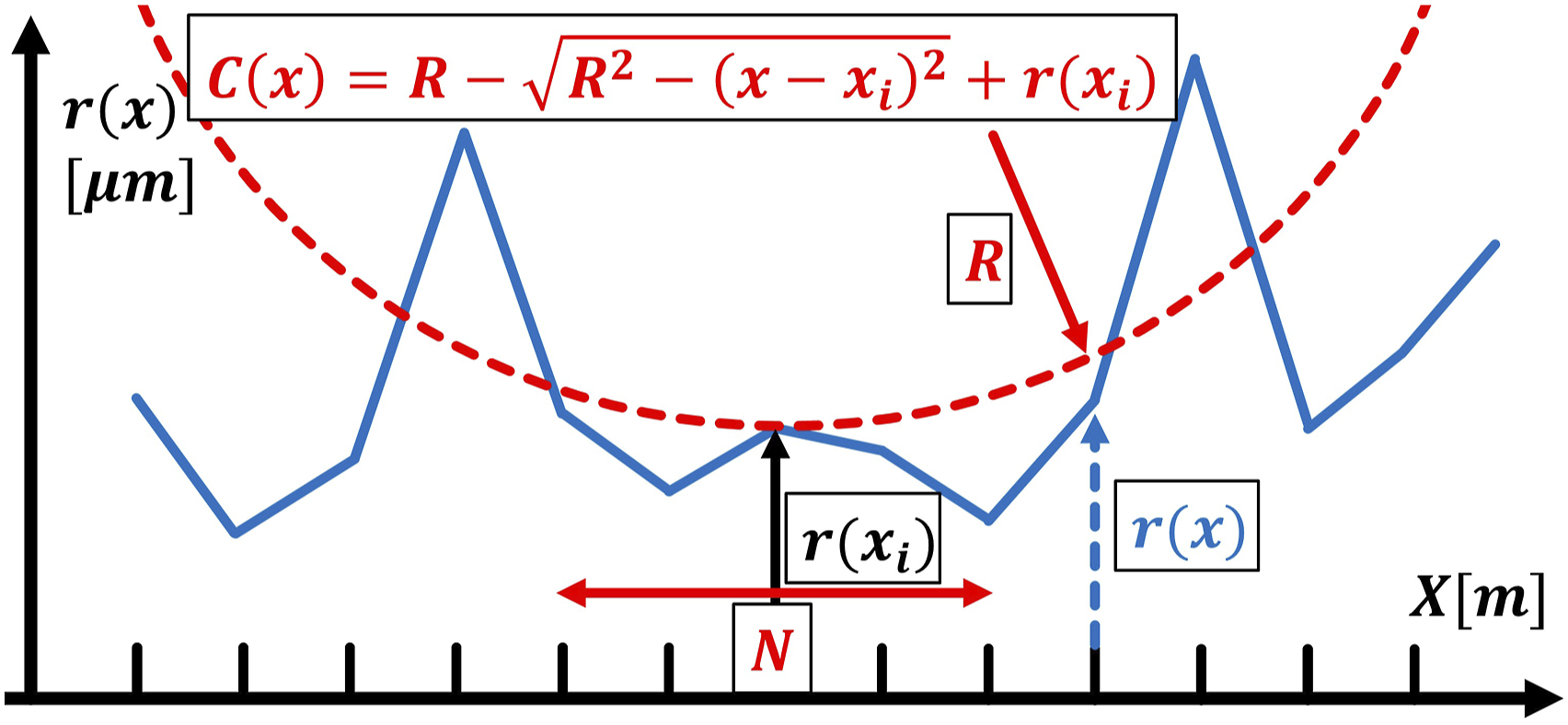
The procedure involves the following steps with (a) Calculation of the first derivative (b) Search for local maxima or minima by searching for a change in sign of the first derivative (c) Check whether the criterion for the second derivative (d) Search for the footpoints (e) Calculation of the width (f) Check whether the ratio of peak height and width is fulfilled. The following criterion serves for this: (g) Repeat the procedure until no new spikes are detected. (7) Curvature correction (Figure 3): Subsequently, the curvature of the wheel must be taken into account. When traversing the longitudinal profile, only those parts of the profile are relevant which the wheel (Radius (8) Calculation of the power spectrum: Based on the longitudinal profile, the power spectral density was calculated as a function of the spectral wavelength. (9) Conversion to one-third octave band spectrum: The power spectral density is converted into a one-third octave band spectrum. This is done according to the specifications of EN 15610.
14
A comparison to the METAS reference is afterwards performed in the wavelength domain. Curvature correction procedure.
Adjustments to the standard
Outlier removal
After importing the data, outliers were removed. This is not part of EN 15610, 14 which only requires discontinuities to be removed. Outlier should be removed before the application of a filter in order not to falsify the result of the filter process. The raw data set was used for this study. A method based on the interquartile range was used as the approach for the numerical implementation. A description of this method can be found in the work of Moska et al. 15
Since the mean value of the data set corresponds to the waviness of the longitudinal profile, outliers that play a role on a roughness value level cannot be detected. It is necessary to divide the data set into segments of data points which are processed individually. The length of a segment is not trivial to define as it is used to determine the mean value and the interquartile range. That determines how many data points are detected and removed as outliers. In order to remove only real outliers, the data set of an undisturbed measurement was used for these investigations. In this case, the deviation from the reference gives an indication of the quality of the outlier removal. The integrated absolute error over the spectrum of acoustic roughness provides a way to assess the deviation.
The integrated error varies between
Bandpass filter
For the acoustic roughness, long-wave signal components as well as measurement noise are not relevant. Therefore, these components are removed by a pre-filter. The process of pre-filtering can influence the result through two main parameters: • Choice of filter technique (e.g. Butterworth, Chebyshev) • Choice of filter frequencies or wavelengths
First, a profile comparison was performed in the time domain. When filtering in the range between Spectrum of acoustic roughness after different filtering.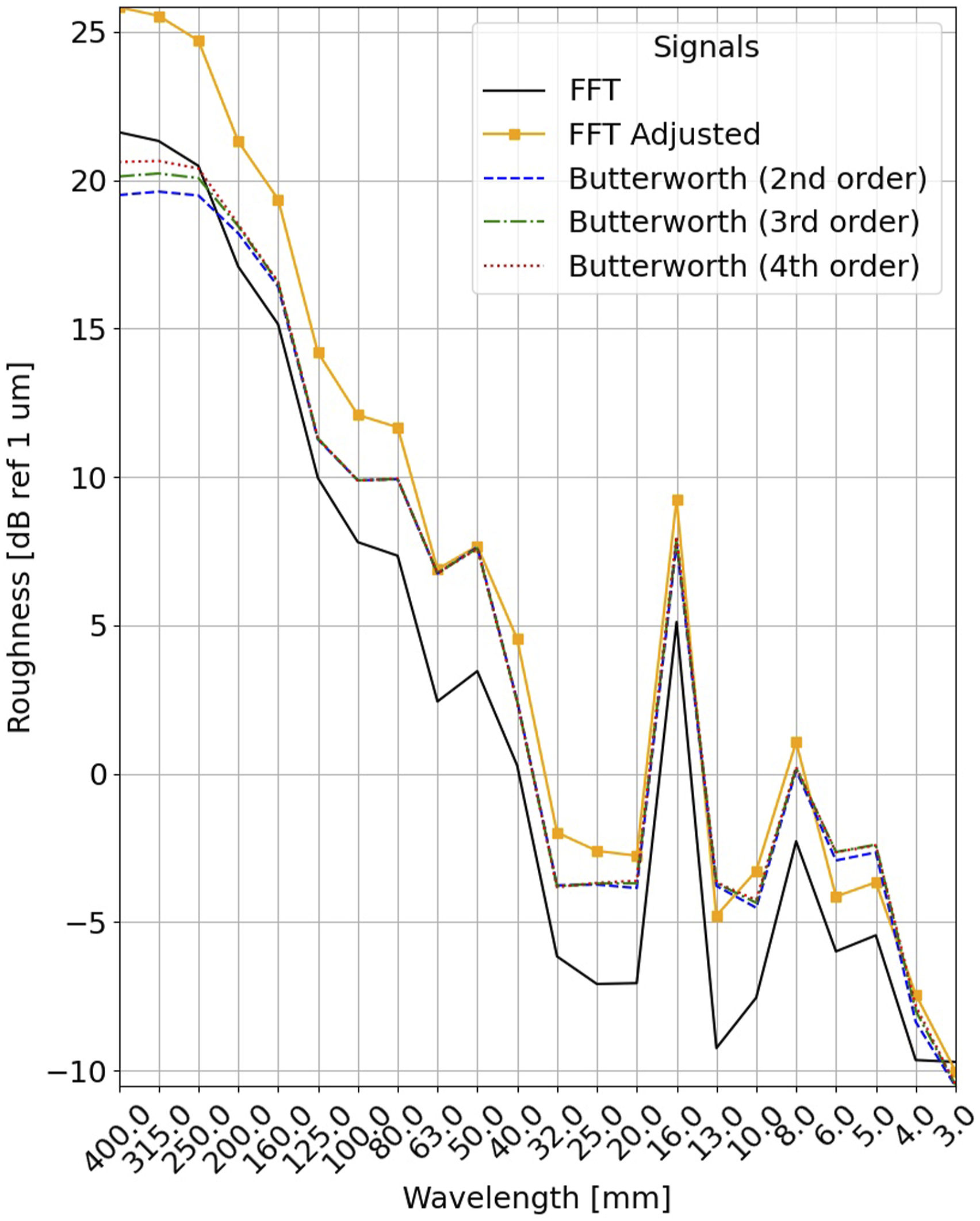
One main difference appears between the Butterworth filters and the manual bandpass filter. Across the spectrum, it can be observed that the absolute values tend to be shifted to higher values with the Butterworth filter. The maximum shift for each filter order is about
Spike removal
The process is shown in Figure 2. Since the method is designed for tactile measurement, the numerical parameters mentioned in EN 15610
14
are not necessarily useful for an optical measurement of the acoustic roughness. In the following, the limit values for the first and the second derivative given by EN 15610
14
were used. The procedure itself is sufficiently defined in the standard. An exception is the definition of the spike height
There are five possibilities to calculate (1) Based on left footpoint: (2) Based on right footpoint (3) Maximal (4) Minimal (5) Based on
Where Spectrum of acoustic roughness for different spike height calculations, measurement with water on the rail.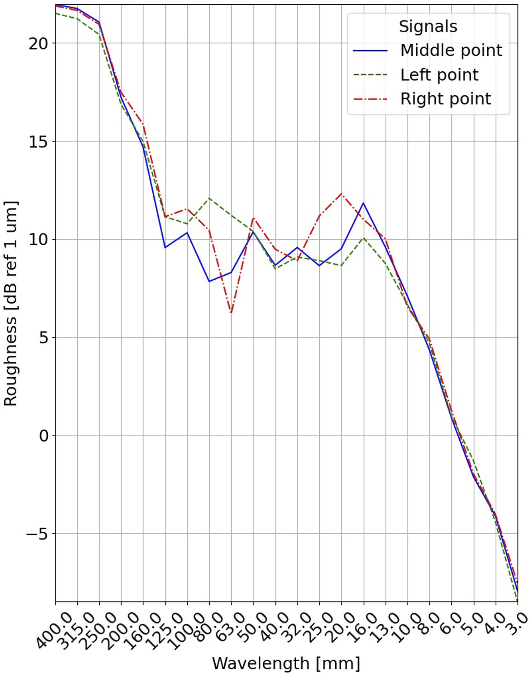
In the case of the definition via the left footpoint, a maximum deviation of
Curvature correction
For each data point
The standard EN 15610
14
does not explicitly specify how many data points Data points within the Hertzian contact zone.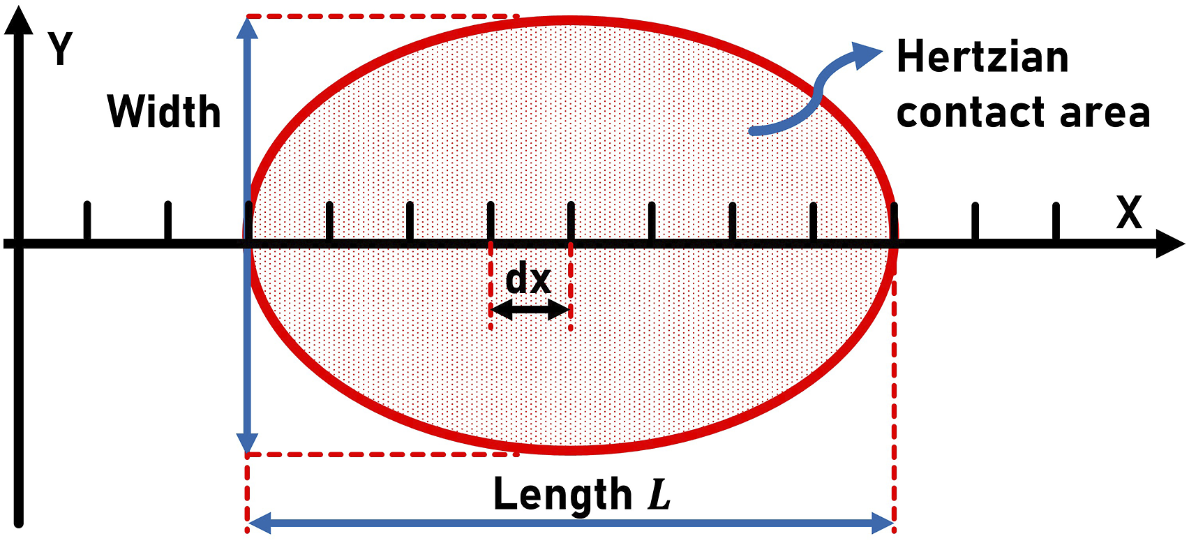
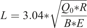
According to Fendrich et al.,
17
the length


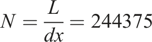
The relevant number of data points for the contact is taken into account regardless of the sampling frequency. Comparing both possible implementations, deviations become apparent depending on the wavelength of the respective band. Figure 7 shows the deviations of the constant point definition of Absolute deviation for 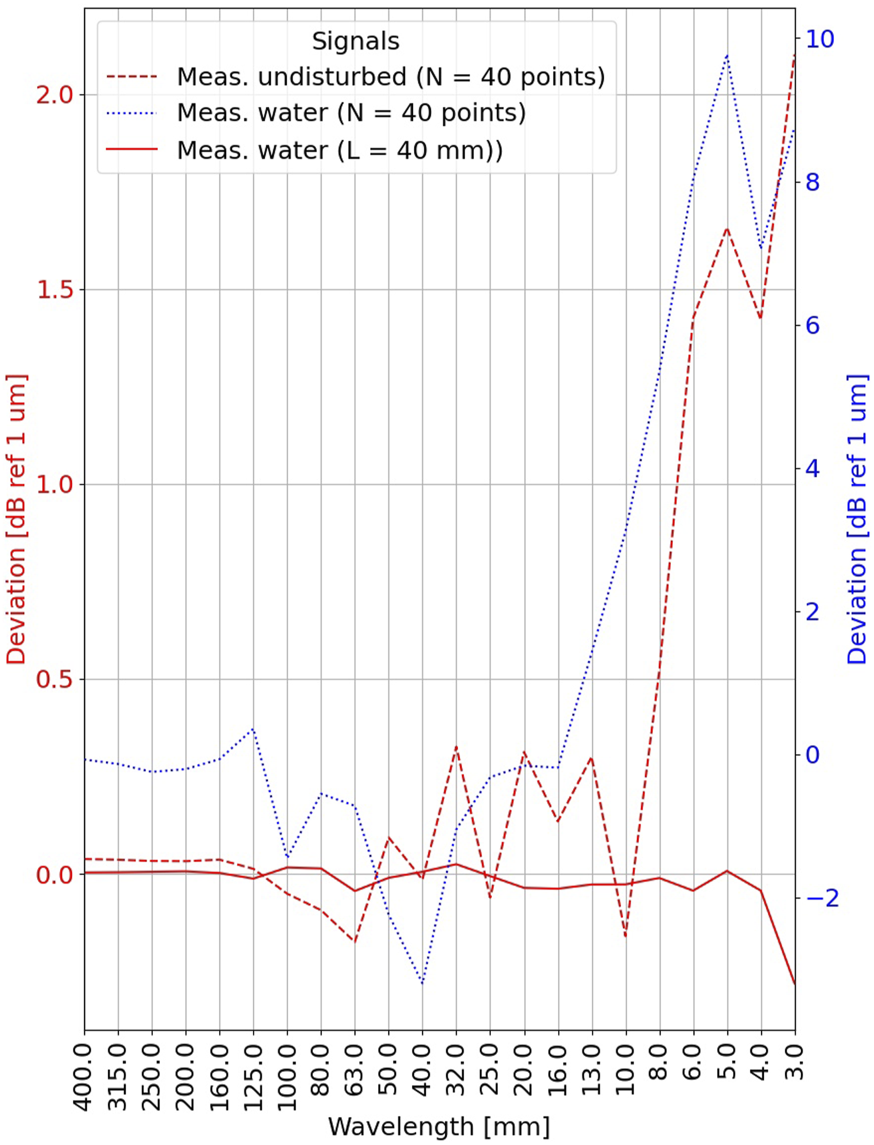
For long wavelengths between
One-third octave band calculation
After calculating the power spectrum, the individual discrete level values are transformed into one-third octave bands. Each individual discrete value is considered as a narrow band of width
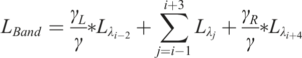
With • • • •
Also specified is the approach how to include narrow bands at the edge of a one-third octave band. These are added to the respective one-third octave band proportionally to their width. The calculation is shown graphically in Figure 8. Shown in red is the range of a single one-third octave band while the narrow bands are shown as bars. In Figure 8, the discrete level values serve as the centre of the narrow bands. This is not explicitly specified in EN 15610.
14
Calculation of the one-third octave band based on narrow bands and central value implementation.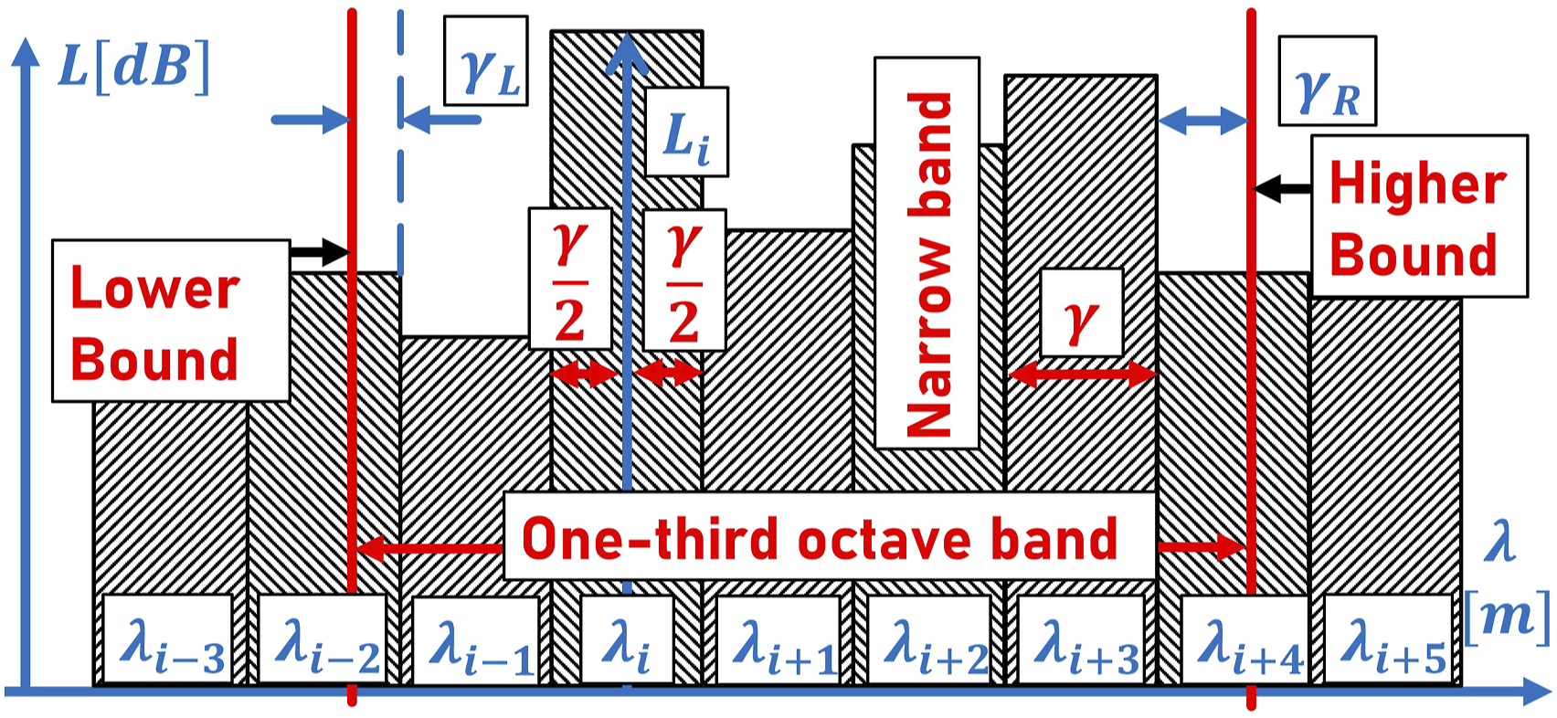
Alternatively, it would be possible to define a narrow band starting from the left edge, which would shift the narrow bands across the width of the spectrum. This alternative is shown in Figure 9. The blue bars correspond to the non-central value implementation of the narrow bands. Calculation of the one-third octave band based on narrow bands and non-central value implementation.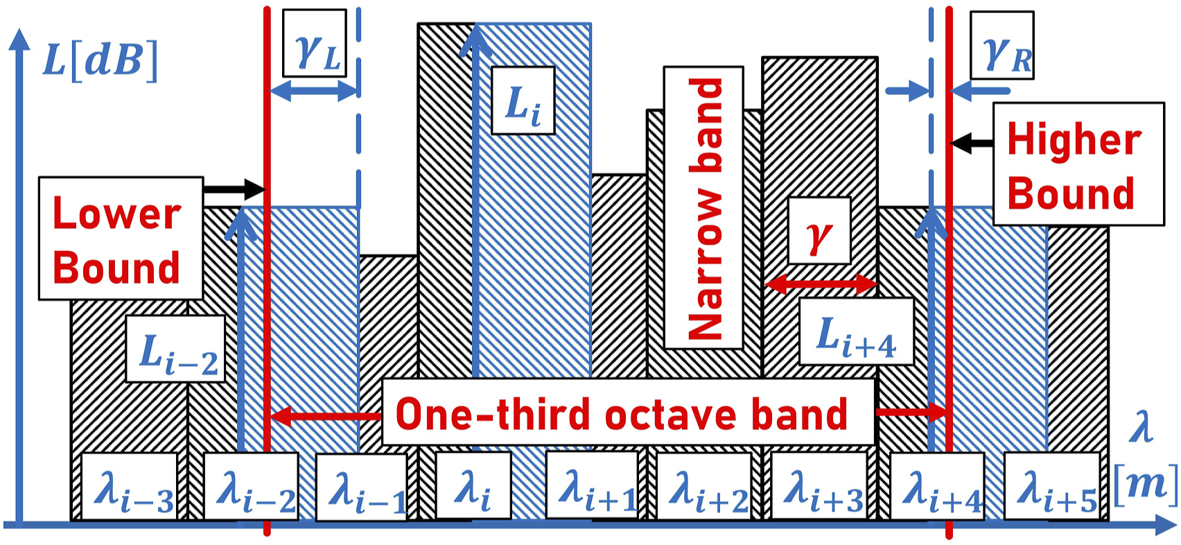
The crucial question is to what extent both definitions affect the spectrum of acoustic roughness. The data was previously processed according to the described processing procedure. Figure 10 shows the spectrum of acoustic roughness for a central value implementation. Spectrum of the acoustic roughness, calculation of the octave band based on narrow bands and central value approach and non-central value approach.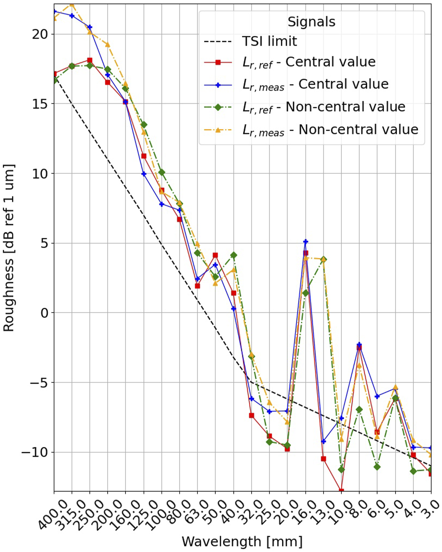
Two peaks are contained at
The absolute value also differs at this point. For the central value implementation, this was
Discussion
Outlier removal
The outlier removal procedure based on interquartile range reliably removed erroneous data points. In a further step, it must be checked for various external disturbances whether this statement can be maintained. In the context of this investigation, it should be examined to what extent a short-term position of the sensor outside its measurement range has an effect on the measurement result. An error signal occurring in this case manifests itself in the measurement data as an outlier and should consequently be able to be removed by this processing step. Furthermore, it should be checked with further measurement data whether a segmentation to
Filter
It is crucial how the measured longitudinal profile data may be processed through a filter before the acoustic roughness is calculated from it. Uncertainties exist both in the use of filter technology (software used) and in the permitted wavelength range in which filtering is allowed in order not to influence the measurement result. Both issues should be addressed to ensure the comparability of different measurements. For a manual bandpass filter, it would also be necessary to determine which window is to be used for the transformation into the frequency range and whether the PSD is multiplied with a correction factor.
Spike removal
It could be shown that the definition of the spike height can already have an effect on the result as long as the measurement data have sufficient disturbances. This deviation cannot be detected for a completely undisturbed data set, which in turn could be attributed to the reduced amount of spikes. It is suggested to calculate the spike height
Curvature correction
It could be shown that the choice of the value for the considered number of data points
One-third octave band calculation
The spectrum of acoustic roughness is strongly influenced by the chosen implementation of the narrow band definition. The result can be influenced simply by the way the narrow bands are computed into one-third octave bands. The problem could be further exacerbated with lower sampling frequencies. The narrow bands would become wider and accordingly have a stronger influence on the calculation in the boundary areas. It is proposed to add a stable definition for this topic to EN 15610 14 in order to prevent deviations of measurements from each other. The approach of defining the narrow bands via the centre point seems robust and allows an implementation that is largely independent of the sampling frequency. In future studies, the calculation of the power spectrum should be considered in more detail and concretized. This aspect was not considered in this study, but could as well have a relevant influence on the result.
Conclusion
Based on the described observations, the EN 15610
14
should be supplemented in several parts. If all the implementation options considered are inserted differently from a calibration measurement, significant deviations in the measurement results can be the consequence. This greatly limits the comparability of the measurements. There is also the theoretical possibility of adapting the measurement result without contravening the current status of the EN 15610
14
standard. A supplement to the standard seems to also make sense in order to establish better comparability between the various measurement approaches. It can be seen that EN 15610
14
was designed for a tactile method. Other measurement approaches are not taken into account. Parameters for the spike removal method are explicitly specified for a tactile tip size of
Footnotes
Acknowledgements
The authors would like to thank the Swiss Federal Office for the Environment (FOEN) and the Swiss Federal Office of Transport (FOT) for the financial support.
Declaration of Conflicting Interests
The author(s) declared no potential conflicts of interest with respect to the research, authorship, and/or publication of this article.
Funding
The author(s) disclosed receipt of the following financial support for the research, authorship, and/or publication of this article: This work was supported by Swiss Federal Office for the Environment (FOEN) and the Swiss Federal Office of Transport (FOT).