A review of techniques for measurement of forces and neutral temperatures in railway track

Abstract

Track failures in the form of thermally induced buckling events or rail breakages on continuously welded rails (CWRs) have long posed challenges for the rail industry. These issues arise because CWRs cannot freely expand or contract as rail temperatures fluctuate during operation, resulting in compressive or tensile stresses. As temperature variations increase, these stresses can lead to rail buckling under compression or separation under tension. Buckling, in particular, poses a serious threat, as it is often associated with derailments, carrying substantial social (rail safety, public perception) and economic (track downtime, damage to freight, rolling stock, and infrastructure) consequences. For this reason, understanding the thermal stress state or neutral rail temperature (NRT) of installed track is critical for rail network owners and operators. This knowledge enables more precise planning of maintenance, targeted rail replacement, and monitoring of high-risk areas. Consequently, there is growing demand for in-situ, non-destructive methods to measure NRT. This paper reviews existing methods for measuring NRT, encompassing approaches developed from the 1960s to the present. Each method is critically evaluated, with the findings summarized in a table that outlines their operational principles, limitations, reported accuracy, and current technology readiness level.

Introduction

Significance of problem

Determination of neutral rail temperature (NRT), the temperature at which continuously welded rails (CWRs) are at zero thermal stress state, has been a prevalent problem since the 1950s. If there were a set of Millennium Prize Problems for engineering, measuring NRT would certainly be on the list.

Historically, railway tracks consist of short sections of rail bolted together with fishplates. The gap between fishplates allows for thermal expansion and contraction of rails at the expense of higher maintenance. Modern rails are continuously welded and typically span kilometres long. They allow for quicker train speeds and smoother rides. However, due to the lack of expansion joints and constraints imposed on the rail, thermal stresses are introduced within the rails, with a lateral component. This poses a derailment risk as hot weather increases the risk of rail buckling whilst cold weather causes pull-aparts.

Between 2018 and 2021 in the United States, rail buckling was responsible for 775 derailment incidents, leading to 14 injuries and a total of $165M in reported damages. This amount accounts for 30% of all reported accident-related damages during that period. ¹ During the summer of 2022, the UK experienced 27 buckles and 3-line closures due to the excessive heat. This was despite imposing speed restrictions at 20, 30 or 60 mph across large proportion of the network and limiting rail use to passenger trains. As climate change intensifies, it is expected that the frequency of rail buckle will increase. Consequently, measurement of rail neutral temperature and rail stress remains one of the top research priorities for US and UK rail administrators. ²

The NRT should always be regulated, and thus maintained within a safe limit to avoid track buckling. Therefore, a device capable of measuring NRT is highly desirable. Over the past decades, destructive and non-destructive technologies (NDT) have been trialled for NRT measurement with varying degrees of success. Most national rail administrators have outlined similar criteria for a suitable industrial solution for NRT measurement ² :

• Accurate, measures the bulk rail stress

• Requires no calibration

• Easy and quick to perform

• Non-contact

This paper presents a comprehensive review of approaches trialled by researchers in the search for a solution for NRT measurement. Initially an introduction is provided for NRT, followed by a summary of different stresses experienced by rail, and a deep dive into the existing approaches for NRT measurement. This is followed by discussion of the methods which includes a summary of the reported field accuracy and technology readiness level (TRL) of existing methods.

Neutral rail temperature

The NRT is defined as the temperature at which the rail experiences neutral or zero stress. In the rail industry, rail thermal stresses are commonly expressed in degrees centigrade (°C), rather than in SI units (Pascals). Over the natural daily temperature cycles, rails are subjected to temperature fluctuations. Track lengths joined with fishplate joints can naturally expand and contract with this thermal fluctuation; continuous welded rail (CWR) unfortunately does not have this luxury. As the rail temperature fluctuates, the linear stress profile of the rail also changes.

When subjected to cold temperatures below the NRT, the rail contracts, creating a tensional force which can lead to cracking and fracture. Fractured rails due to pull-aparts are generally less of an issue if they are detected early and appropriately managed by repair, temporary support and speed restrictions. The Federal Railroad Administration ³ noted that if the rail is properly anchored, the pull-apart gap is typically less than 4” (25.4 mm) and that trains can still traverse this gap relatively safe compared to large, buckled rail. Additionally, crack propagation can be detected by industry standard NDTs such as ultrasonic inspection, and the failure may also be detected by the signalling system. Despite this, the damaged region will deteriorate with operation due to the wheel-rail impact, but it does not normally induce derailments or large damage. ⁴

In excessively warm conditions above the NRT, the rail attempts to expand, leading to compressive forces which, when exceeding a limiting stress, can cause buckling of the rail. Buckling occurs when internal stresses continue to increase leading to two possible static equilibrium scenarios: non-deformed state or laterally deformed state. The exact moment of buckling, and the required force, depend on the lateral resistance that can be provided by the sleepers in the ballast. If the lateral resistance is no longer sufficient to prevent sideways movement, buckling will occur. The relationship between thermal stress and rail temperature is defined as follows:

$∆T=\left(T_N-T_R\right)=\frac{\sigma }{E\alpha }$

(1)

where $T_N$ is the NRT, $T_R$ is the current rail temperature, $∆T$ is the temperature difference between $T_N$ and $T_R$ , $\sigma$ is stress, $E$ is elastic modulus and $\alpha$ is the thermal expansion coefficient. When $∆T$ is positive, the rail is in tension and conversely when it is negative, the rail is in compression. The NRT, $T_N$ can be calculated from the temperature change summed with the rail temperature:

$T_N=∆T+T_R$

(2)

Substituting equations (1) into (2) gives:

$T_N=\frac{\sigma }{E\alpha }+T_R$

(3)

If the rail temperature drops below the NRT, equation (1) demonstrates that the stress is positive, meaning the rail is subjected to a tensional force as it tries to contract, and according to equation (3) there is an increase in NRT. Likewise, if the temperature increases above the neutral rail temperature, the rail tries to expand and is therefore under compression. Naturally, the NRT of the rail reduces to counteract this compressional force.

Managing neutral rail temperature

The NRT is localised depending on the ambient conditions where the track will operate. For example, in the UK the NRT is set to 27°C, as this is considered an optimum NRT to balance the risk of breaks and buckles. On Australia’s Darwin-Alice Spring line, where ambient conditions can reach 50°C, the NRT is much higher. ⁵ Therefore, the main maintenance strategy of NRT is preventative; track is installed when ambient conditions are as close as possible to the desired NRT. ⁶ Rails are not normally installed when the ambient temperature is above the NRT. If the ambient temperature is too low during installation, the tracks are typically stretched to impart a tensional force which compensates for the compressional force due to expansion which will occur when the ambient temperature increases. ⁶ Adjustments are therefore made in the form of imparting stress to the track to ensure the NRT is as close as possible to the “true NRT”, which is between the minimum and maximum ambient temperature conditions.

To complicate matters further, there will be NRT variations along the length of track at the point of installation. Some points along a track will naturally incur higher daily temperatures due to instances such as more sunlight exposure compared to a section of CWR under shade. Additionally, over the course of the rail’s lifetime there are further fluctuations, the causes of which are reviewed by Skarova et al. ⁷ The authors explain that NRT can vary due to thermal fluctuations, inadequate longitudinal restraints, changes in track settlement and also acceleration and braking forces of trains. These factors alter NRT by changing the track length and subsequently its stress state.

NRT should always be regulated, and thus maintained within a safe limit to avoid track buckling. If a track is deemed to have a NRT that differs significantly from other sections of the track, then an adjustment must be carried out. This is typically conducted by either stretching or cutting the rail, similar to the installation process mentioned above. For rail administrators, a quick, reliable, and non-disruptive measurement solution is highly desirable to facilitate this rail management process.

Rail variants

Prior to discussing measurement techniques, it is important to understand the rail variants existing in operation and how they are processed. This section thus covers the typical types of rails employed in the UK and Europe, and how they are manufactured.

Types of rails

Railway tracks are typically expressed in weight/length. In Europe, rails are measured in kg/m whereas the US employs lbs/yd units. Prior to the introduction of the European standards, most railways had their own legacy sections, in the UK these included 113 lb/yd, 110lb/yd and 95lb/yd bullhead rail. Since then, Europe has standardised rail sections that can be used and they are always described in kg/m. Many of the modern lines use 60E1 or 60E2. However, a wide range of different sections are still in use across Europe which are described in EN 13674. ⁸

For rails, steel grade designation number that is Grade 260 refers to the Brinell hardness of the steel. ⁹ Since 2004, over 90% of newly installed UK rail networks are of R260 grade. This grade is also widely used in continental Europe.

Steel rail processing

The process of producing high quality rail steel has progressed steadily over the decades, eliminating gasses, reducing segregation, inclusions, pipe, and other manufacturing features that could adversely impact the rail during its operational life. ⁹ Rail steel needs to have tightly controlled residual elements including phosphorus and the base metals and so it requires the use of high-quality scrap, iron ore or direct reduced iron to control the residual elements.

The two main process routes are used for rail steel manufacturing are:

(a) The blast furnace - basic oxygen converter process. The blast furnace converts iron ore into pig iron by reducing the iron oxide at high temperature with carbon. The pig iron is fed into a basic oxygen converter where carbon is removed from the pig iron by oxygen to produce steel.

(b) The electric arc furnace process. This process melts scrap steel or direct reduced iron with electrical energy to produce steel.

The liquid steel from both process routes requires secondary steelmaking to modify the composition to the precise requirements of the grade that is being produced. Vacuum degassing ¹⁰ is used to remove gases such as hydrogen, which must be limited to a very low level to eliminate the risk of hydrogen shatter cracks forming in the rails.

The refined steel is solidified in a continuous casting machine ⁹ to produce blooms that are suitable for rolling into rails. When casting operation starts, nozzle at the bottom of the ladle opens and steel flows under a controlled rate into the tundish and from the tundish through submerged entry nozzles into one or several moulds, where it undergoes its first solidification at the metal/mould interface. As the solidifying steel exits the mould it is drawn through the caster using a series of rollers and spray cooled with water, the thickness of the solidified shell increases progressively. At the end of the machine, the strand is cut to produce a bloom of the precise weight that is required to make a specified rail section and length.

Rail blooms are transferred to the rolling mill where they are reheated to rolling temperature (around 1200°C) before passing into the rolling mill. Scale removal before and during rolling is essential to ensure the integrity of the rail surface and to avoid rolling the scale back into the rail. There are many different rolling mill designs that can produce rail, but most adopt a universal approach to at least part of the rolling process as this is generally considered the most rapid and precise method to form the rail shape.

The rolled rail is cooled and then roller straightened to create a flat straight rail. This process bends the rail over multiple rollers in both vertical and horizontal directions. Initially a high percentage of the rail section experiences plastic deformation, this reduces to very low levels of plasticity towards the end of the machine. This combination of plastic bends creates substantial residual stresses in the rail. Other processes including cooling, heat treatment and end straightening also influence residual stress in the rail.

Modern rail manufacturing facilities are designed to produce highly consistent rails that are free from manufacturing imperfections that could influence in service performance. Internal quality is largely determined during the bloom manufacturing processes; the internal integrity is confirmed by ultrasonic inspection of the whole rail. Surface integrity is largely defined during the hot rolling and cold finishing processes. All surfaces are checked for cracks and scratches that could become stress raisers in service. Eddy currents and visual methods ⁹ are used to confirm surface integrity. Dimensional accuracy is another critical factor, automatic dimensional inspection is carried out to confirm the key dimensions along the entire rail length. In combination the production and inspection of rail has developed to a level where the manufacturing defects should not impact the service life of rail. The improvement in manufacturing capability of rail has been built into the major rail specifications to eliminate manufacturing features as a major cause of premature rail failure.

Most rails last for decades with average life of around 30 years. ¹¹ This is extremely variable depending on the intensity of use and so it is not uncommon for rails to be over 50 and even 75 years old. Consequently, there remains a legacy of rails in service that have not been produced to the modern standards. Isolated defects are still found from legacy manufacturing faults such as tache ovals caused by hydrogen cracking, ¹² that has since been eliminated by the move from ingots to continuously cast steel and the introduction of vacuum degassing.

Local stresses in rail

Rail neutral temperature is dependent on the net force over the cross section of the rail. Locally, however, the stresses vary significantly due to the addition of local stress effects as well as stresses from external sources such as trains. These include residual, welding, bending and contact stress.

Residual stresses in rail

Majority of the residual stresses in rail are generated during the cold roller-straightening process. ¹³ As the rails cool, they bend. To correct for unwanted bending, rails are straightened by passing them through a series of roller. During this process, they undergo plastic deformation due to the alternating bending stresses. Residual stress patterns from rolling and cooling are largely replaced by the cold roller-straightener stresses.

Heat treatment prior to roller straightening increases the yield strength of the rail. Subsequently, a larger force is necessary to be imparted during cold roller-straightening and the end result is higher residual stress in the rail. ¹⁴

During the service life of a rail, stresses are accumulated on the rail head due to repeated rail wheel rolling-contact. These dynamic contact forces are high and can cause plastic deformation around the contact surface and modify the residual stress field on the running surface and internally within the rail head.

Naumann ¹⁵ stated that for cold roller-straightening, the contact pressure between the rail and rollers is responsible for the residual stress pattern. He argued that the special cross section with the wide head and foot and the slim web is the reason for the typical residual stress distribution. An alternative explanation is that the residual stress distribution can be attributed to the interface between plastic and elastic deformation as the rail is bent over each straightening roller coupled with the direction of the last plastic bend, which forces residual stress towards the head or foot.

The residual stresses are partly tensile and compressive across the rail section and therefore do not add to the resulting force over the cross section. However, any NRT measurement methods that measures from the side of the rail (instead of top-down) would need to consider the varying residual stresses across different parts of the rail. Figure 1 shows the typical residual stress distribution across a rail’s cross section. A tensile stress is typically present between 100 and 200 MPa in the rail head as well as rail base whereas the rail web experiences a compressive residual stress. It is reasonable to assume that the residual stress at the base of the foot contributes to foot fatigue failures; and the tensile head stresses may contribute to rolling contact fatigue, although this depends on the stress shakedown in use and deformation of the running surface which tends to relieve the residual head stress with the passage of traffic.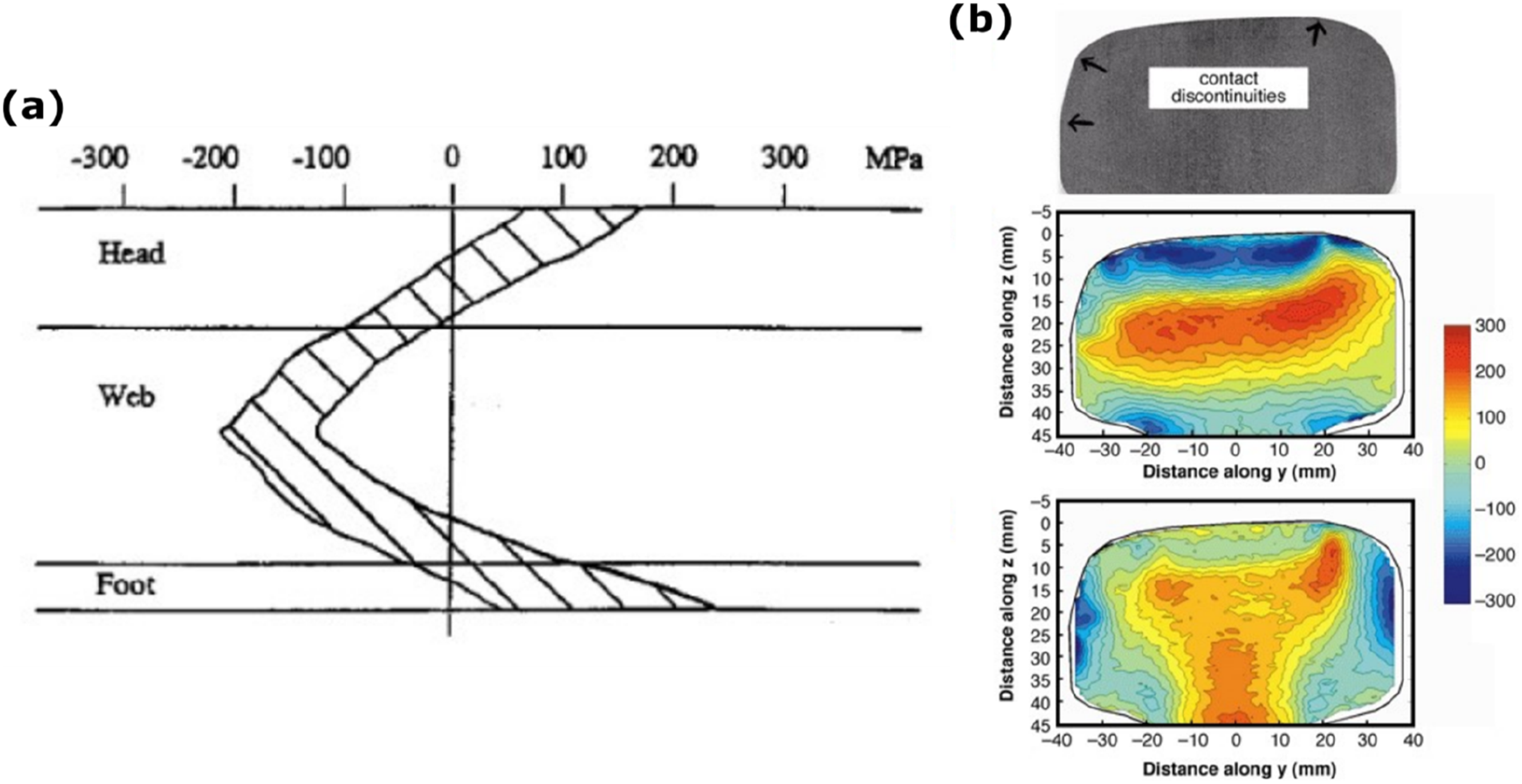

Figure 1.

Variation in residual stress across the (a) rail head, web, and foot ¹⁶ and (b) rail head due to rail-wheel contact. ¹⁷

Welding stress

Aluminothermic welding (ATW) is the most common weld type used in joining CWR. Within the weld, the web section of the rail weld is strongly in tension in both longitudinal and vertical components, ¹⁸ unlike typical rail which is in compression within the web region. This can lead to crack initiation and propagation if there is porosity or inclusions in the weld section. ¹⁹ The residual stress resulting from a weld can influence track up to 0.5 m away from the weld location, thus impacting the total stress state of the rail in this region. ²⁰ The weld residual stress can be mitigated if the weld operation is performed before the track is clamped to the sleepers. Overlay welding, a secondary weld process, is used to repair rail head damage, but is not an ideal solution and can lead to fatigue crack growth, particular for the shallower repairs which have a 30% higher stress value compared to deeper welds. ²¹ Weld finish can also impact the loading conditions with dipped profiles causing the greatest dynamic loads. ²² However, dipped welds are not controlled as well as peaked welds during installation. This loading stress impact is discussed in §1.5.4. As welding stresses is unlikely to impact stresses 0.5 m away, welding is a minor factor and where possible NRT measurement should be conducted at least 0.5 to 1 m away from welds.

Bending stress

Where the track has to curve to avoid geographical features, a bending stress is introduced into the track. Bending stress is influenced by the rail width and radius of curvature. Assuming elasticity and using a Young’s modulus of 2.07 GPa, with a typical rail half width of 70 mm and a curve radius of 400 m, the maximum bending stress is approximately 40 MPa which is in the same order of magnitude as thermally induced stress. However, since most of the stress will be concentrated on the flange tips, NRT measurement methods that circumvent the region, that is measuring through the rail web, can operate freely without being influence by bending stresses.

Contact stress

Plastic deformation occurs when rail loading exceeds the yield stress of the material, resulting in an inherent residual stress upon the removal of the load. Cyclic loading can then potentially alter the residual stress. ²³ As such, rail-wheel contact results in contact residual stress, in the direction parallel to the running surface and penetrating up to 20 mm into the rail head. ²⁴ These stresses from passage of traffic relieve the high tensile longitudinal residual stresses from roller straightening. Consequently, old rails are vertically bent when removed from service as the foot stresses from manufacture remain, but the head stresses have been reversed from passage of traffic. Thus, variation of residual stress in rail heads needs to be accounted for in NRT measurements. Despite this, residual stress due to manufacturing processes and in particular, roller straightener design and settings as detailed in §1.5.1, remains the key contributor of residual stresses in rail and can have a significant impact on the levels and balance of the residual stresses in rail. These variations must be considered when developing a non-destructive measurement device for thermal stress.

Track-bridge interaction stress

Railway tracks laid across bridges are subjected to additional stresses from the relative movement between the track and bridge.^25,26 This occurs due to temperature changes of the bridge deck sections, traction of braking forces from a passing train and bending of bridge deck sections under vertical loading.^26,27 As ambient temperature fluctuates, bridges by design are able to freely expand or contract whilst CWRs are constrained, imparting thermal stresses in them. The relative movement of the bridge beneath the static railway track imparts additional stresses onto the track through the fasteners. ²⁶ This needs to be accounted for when measuring NRT across tracks laid on bridges as they are of the equal order of magnitudes. Effects from train traction and deceleration can be circumvented by withholding measurements when trains traverse through the bridge.

Measurement techniques for NRT measurement

This section provides a comprehensive summary of the existing measurement techniques for determining thermal stress or NRT. These range from simple extensor style methods to complex, mathematical acoustic techniques at various level of maturity and accuracy.

Rail cutting method

Prior to 2003, the rail cutting technique was widely utilised. The rail cutting method^4,28–30 is a destructive method which utilises, the cutting of rail to release the residual thermal stress and then measuring the elongation to deduce the NRT within the rail. Rail is untightened from sleepers and is severed using gas cutting equipment which releases the thermal residual stresses, resulting in the expansion or contraction of rail. The change in rail length is then measured and converted to NRT.

The procedure of rail cutting method is illustrated in Figure 2. Prior to cutting of rail, the cutting location is identified, required to be at least 50 m from the end of a CWR rail or from a switch. Punch marks are introduced at both sides of the cutting location, roughly at 100 mm apart. The distance between punch marks and rail temperatures are measured before and after the rail is cut. Elevating the unclipped rail length on rollers ensures that contraction is not restricted by friction between the rail/pads and sleepers. The NRT, $T_N$ rail temperature, $T_R$ and elongation, $e$ can be related through the following relationship, where $L$ is the rail length over which stress relaxation occurs and $\alpha$ is the coefficient of rail expansion.

$e=\alpha ·L·\left(T_N-T_R\right)$

(4)

Figure 2.

Rail cutting method for deducing rail thermal stress/NRT.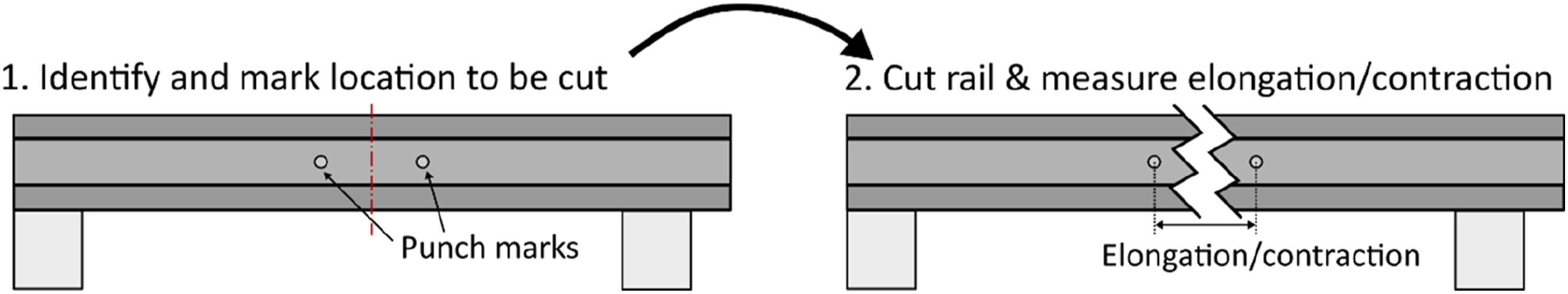

The primary challenge lies in obtaining an accurate stress relaxation rail length, $L$ . Field measurements show that the rail relaxation length varies non-linearly with NRT. This was thought to be due to the varying number of sleepers influencing the force equilibrium as rail temperature increases from NRT, which subsequently increases the rail length involved.

Despite this, accuracy of the method is good, quoted at ±2°C or ±5.2 MPa for UIC-60 rails. ⁴ Errors up to 15°C however were reported, ³⁰ especially when the stress relaxation rail length is not accurately measured.

The method is also relatively straightforward, requiring only gas cutter and temperature and position measurement kits. However, the method is labour intensive, requires track closure, suffers from lengthy measurement time limiting track availability and cost comparatively high per measurement point due to requirement for track closure.

Rail lifting method

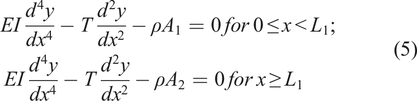
The rail lifting method,^31,32 first documented in 1987 ³¹ is the industry standard for determining the NRT for CWR. It is commercially known as Vertical Rail Stress Equipment (VERSE), supplied by Pandrol Ltd based in Plymouth, UK. The method is based on the relationship between the tensile or compressive force in the rail and the force required to displace the rail a certain distance. The larger the thermal stress, the higher the force necessary to deflect the rail. It can be modelled as a beam connected with heavier beams as demonstrated in Figure 3, ³² where $E$ is the modulus of elasticity, $I$ is the moment of inertia of rail, $T$ is the tension in rail, $x$ is the position, $y$ is the deflection and $\rho A$ is the rail weight per length.

$EI\frac{d^{4}y}{d{x}^4}-T\frac{d^{2}y}{d{x}^2}-\rho A_1=0\hspace{0.17em}for\hspace{0.17em}0\le x<L_1;\hspace{0.17em}EI\frac{d^{4}y}{d{x}^4}-T\frac{d^{2}y}{d{x}^2}-\rho A_2=0\hspace{0.17em}for\hspace{0.17em}x\ge L_1$

(5)

Figure 3.

Model of a beam connected with adjacent heavy beams (adapted from ³³ ).

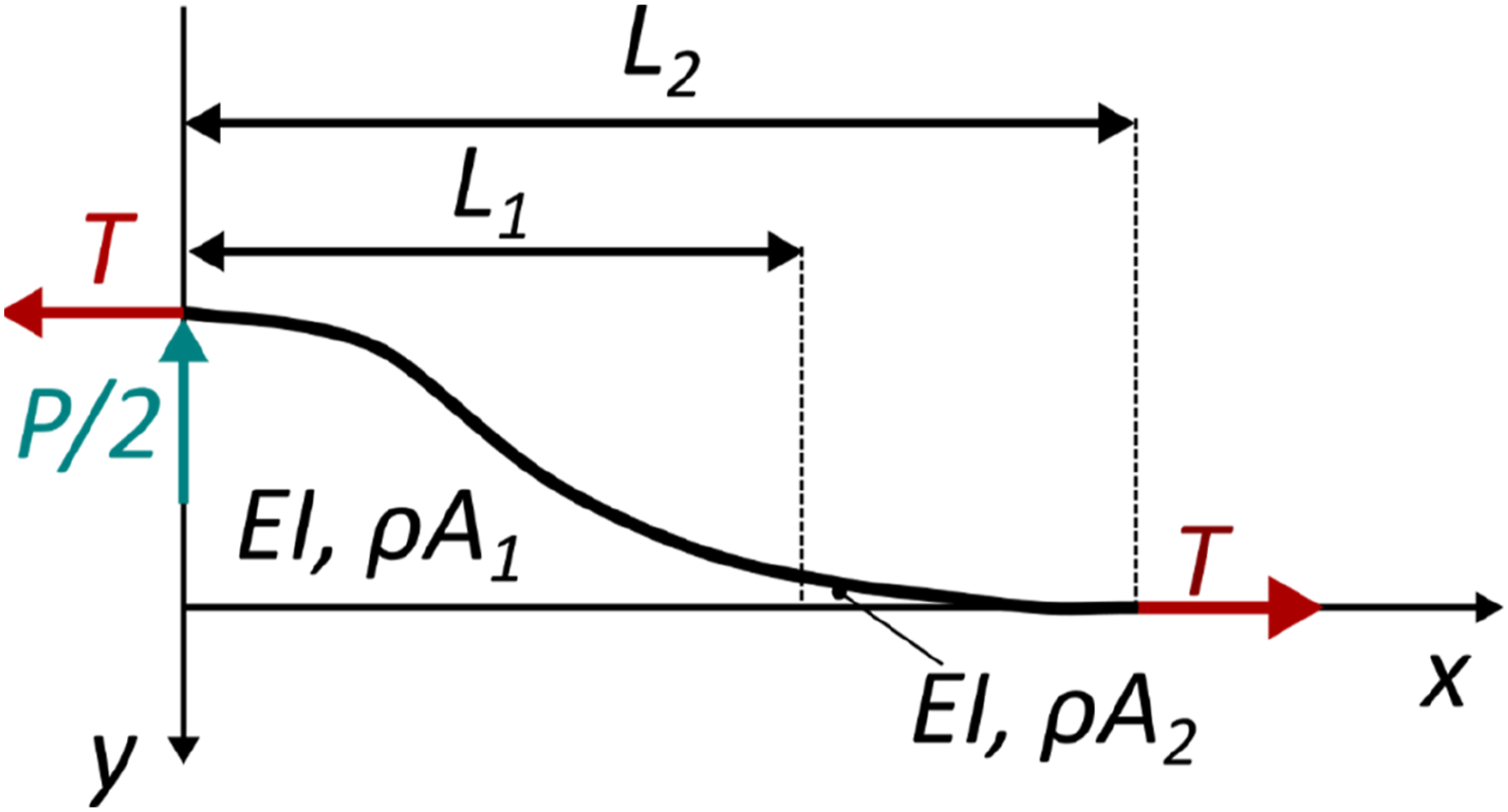
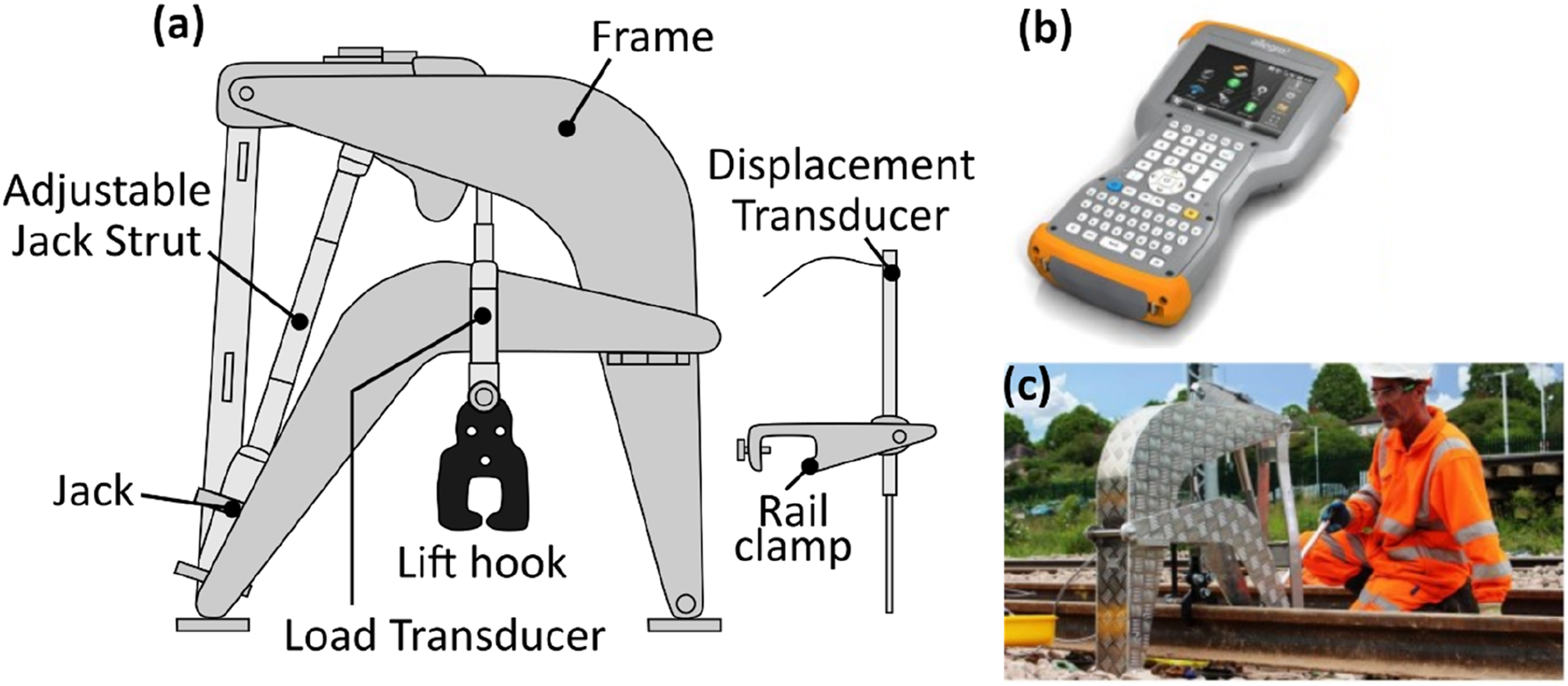
The VERSE system,^30,34 shown in Figure 4, consists of a clamp to lift the rail head with its built-in hydraulic jack. Measurement involves unclipping 30 m of rail track, elevating the rail onto two simple supports positioned 10 m away at both sides of the centre point and applying deflection by incrementally lifting the rail head through the hydraulic jack up to 10 kN. As deflection is applied onto the rail, the force and displacement profile were captured. The NRT, $T_N$ is then calculated using equation (6) where $T_a$ is the ambient temperature, $F_{start}$ and $F_{end}$ are rail loading applied at the start and end of the measurement, $\alpha$ is the coefficient of expansion, $A$ is the rail cross-sectional area and $E$ is the rail modulus of elasticity. This is done through a handheld interface after consideration of geometric properties, rail wear, and track curvature.

$T_N=\frac{\left(F_{start}+F_{end}\right)}{2\alpha AE}+T_a$

(6)

Figure 4.

VERSE NRT measurement system: (a) Mechanical structure, (b) handheld device for NRT calculation, (c) system in action. ³⁵

The method has a verified accuracy of ±3.5°C^4,34,35 or ±8.3 MPa with a relatively rapid measurement time of one measurement per hour and easy to operate interface in the form of a handheld computer. In 2007, Pandrol claims to have sold 100 systems globally with the UK being their largest market. ³⁰ Despite this, the method has several limitations. As 30 m of railway track needs to be unclipped, the method is unsuitable under tight arrangements and cannot be used for rail under compression as the untightened rail will buckle. The method is also unsuitable when rail temperature is considerably larger (>28°C) than the NRT ³⁰ as the rail will either buckle or pull-apart upon unclipping. The method is also limited to straight tracks or rail with a radii larger than 700 m as its accuracy quickly deteriorates for radii smaller than 700 m.

Hole drilling method

The hole drilling method, first introduced in 1934, ³⁴ is an ASTM certified method ³⁶ for measurement of residual stresses in components. As the name suggests, the method is fairly destructive which involves introducing a bore on a component and measuring the change in surface strains around the introduced feature. The bore can be through or blind with a depth typically equal to its diameter and small compared to the component thickness. ³⁷ As material is removed, the component’s stress state undergoes a change to re-attain its residual stress equilibrium. Strain gauges are typically employed for measuring the strain variation around the proximity of the bore with special standardized rosettes available commercially for this. ³⁷

For a through-hole within a thin infinite linear elastic plate subjected to biaxial residual stress, ${\sigma }_{r-x}$ and ${\sigma }_{r-y}$ , the relieved radial strain at a certain point $P\left(R,{\alpha }^{\prime }\right)$ can be represented as shown in equation (7) where $R$ is the radius, ${\alpha }^{\prime }$ is the angle in the cylindrical coordinate, and $\stackrel{\sim }{A}$ and $\stackrel{\sim }{B}$ are constants defined in equation (8) dependent on $E$ , $v$ and $r$ , the Young’s modulus, Poisson’s ratio, and ratio between arbitrary radius from hole centre, $R$ to the hole radius, $R_o$ . ³⁸ Since three unknown are present ( ${\sigma }_{r-x}$ , ${\sigma }_{r-y}$ , ${\alpha }^{\prime }$ ), three independent measurements of radial strain are required to compute the stress. As such, three strain gauges are typically mounted at various angle relative to one another around the site of the hole prior to drilling.

${\epsilon }_r={\sigma }_{r-x}\left(\stackrel{\sim }{A}+\stackrel{\sim }{B}\mathit{cos}\mathit{cos}\hspace{0.17em}2{\alpha }^{\prime }\hspace{0.17em}\right)+{\sigma }_{r-y}\left(\stackrel{\sim }{A}-\stackrel{\sim }{B}\mathit{cos}\mathit{cos}\hspace{0.17em}2{\alpha }^{\prime }\hspace{0.17em}\right)$

(7)

$\stackrel{\sim }{A}=-\frac{1+v}{2E}\left(\frac{1}{r^2}\right),\stackrel{\sim }{B}=-\frac{1+v}{2E}\left(\frac{4}{1+v}\right)\frac{1}{r^2}-\frac{3}{r^4}$

(8)

Conversely, for a blind hole, the stress state varies in a complex manner which necessitates the replacement through-hole of coefficients $\stackrel{\sim }{A}$ and $\stackrel{\sim }{B}$ with their blind-hole counterparts, $\underset{¯}{A}$ and $\underset{¯}{B}$ which is a function of dimensionless hole depth $Z/D$ in addition to $E$ , $v$ and $r$ . These coefficients can only be computed either experimentally^37,39 or through finite element methods.^40,41

Researchers from University of California San Diego (UCSD)^41,42 have successfully implemented the hole drilling method for rail thermal stress measurement on US AREMA 136RE and 141RE rails. They initially conducted FE studies to obtain the blind-hole calibration coefficients $\underset{¯}{A}$ and $\underset{¯}{B}$ which they subsequently validated through uniaxial testing of an aluminium bar instrumented with strain gauges. Measurements were subsequently carried out on unconstrained and constrained 136RE and 141RE rail sections, with the latter conducted at UCSD’s large-scale buckling test bed. A 3 to 4.1 mm bore was introduced at increments of 0.1 mm at the centre of the rail web for a total depth of 2 mm or 1/10th of the total web thickness. Measurements from the unconstrained rails were used to estimate the longitudinal residual stresses present in the rail which was subtracted from the total measured stress in the latter constrained tests to yield thermal stress. Errors were reported at ±5°C or ±13 MPa during the initial study ⁴¹ which was improved to ±3.8°C or ±9.7 MPa through subsequent measurement refinements. ⁴² The accuracy of the method primarily depends on the assumed relationship between longitudinal and vertical residual stresses and the calibration coefficients $\underset{¯}{A}$ and $\underset{¯}{B}$ . Despite proven to yield satisfactory accuracy, the introduction of a shallow bore at each measurement point would eventually be an issue as an agglomeration of these could eventually compromise the integrity of rail networks. This method also requires track closure for the pneumatic drill assembly and strain gauges to be installed at the rail web and measurements taken.

Deformation techniques

Deformation-based techniques centre around inferring rail forces from deformation of rail which includes strain or deflection measurements. Multiple methods exist for strain measurements in rail, these include resistive strain gauges, displacement, fibre-bragg sensors and more recently Digital Image Correlation (DIC).

Resistive strain gauge

A resistive strain gauge produces an electrical signal proportional to the mechanical strain of the surface which they are bonded. ⁴³ They can be made extremely small and can be attached to components of any share which may be moving. It measures strain through a change in resistance within the gauge. The resistance, $R_c$ varies with, ${\rho }_c$ the resistivity of the material, $L_c$ the length and $A_c$ the area of the conductor. When a material is subjected to strain, the resistivity changes due to changes in one or all of the variables.

$R_c=\frac{{\rho }_c{L}_c}{A_c}$

(9)

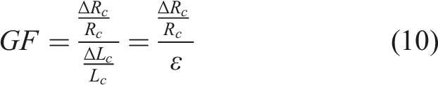
In a typical strain gauge, as illustrated in Figure 5(a), the conductor is looped into a grid pattern, called the resistive foil, and mounted on a flexible, insulating backing layer which then bonds onto the component of interest. ⁴⁴ As such, the strain gauge measures an averaged strain across the grid pattern and the sensitivity of the strain gauge is dependent on the grid material, commonly made of out Nickel-Chromium (Nichrome) or Nickel-Copper (Constantan) alloys. Each grid material has a different gauge factor (GF), defined as the unit resistance change per unit strain as mathematically represented in equation (10). Nichrome and Constantan gauges have a gauge factor of around 2.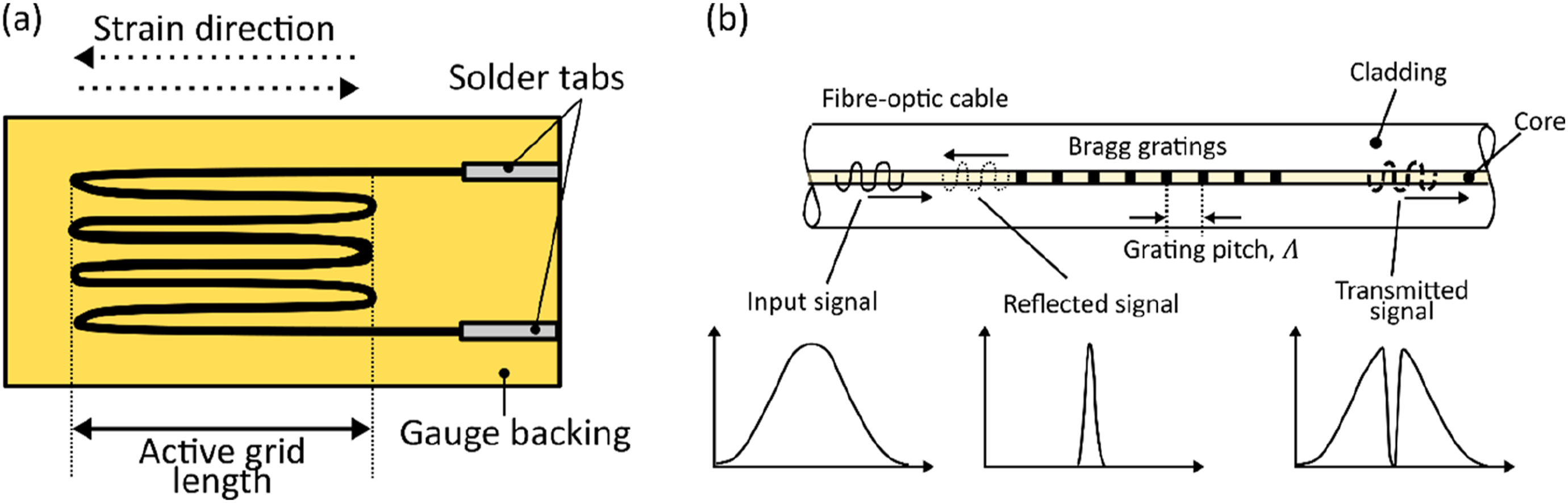

$GF=\frac{\frac{∆R_c}{R_c}}{\frac{∆L_c}{L_c}}=\frac{\frac{∆R_c}{R_c}}{\epsilon }$

(10)

Figure 5.

Schematic of (a) a typical resistive strain gauge ⁴⁴ and fibre-bragg optical sensor. ⁴⁶

Through measuring the strain, assuming that the material is linearly elastic, the stress can be calculated through Hooke’s law. Electrical resistance however also depends on temperature and as such temperature compensation needs to be performed. It is prudent to note that, since the measuring grid is bonded onto the specimen’s surface, the measured strain is surface strain and as such the calculated stresses are surface stresses.

Liu et al. ⁴⁵ proposed a bi-directional strain method for NRT monitoring. They stipulated that the transient nature of CWR variation during operation cannot be sufficiently quantified through uniaxial strain measurements. The proposed sensor consists of a H-shaped steel plate and a full-bridge strain gauge to measure longitudinal and transverse strain. The strain gauges are installed at the thinner section of the plate, whilst the thicker ends are bolted onto the rail. Material of the plate has the same thermal properties as rail. Despite this, due to the non-uniform sectional area between the strain gauge section and the outer plate region, correction factors are necessary. Since both ends of the plate is fixed onto the rail web through bolts, the system necessitates drilling into the rail web. Assembly also consists of a thermocouple for ambient temperature measurements. The authors validated the device through two tests: by constraining a 600 mm CHN60 rail within a 1 MN testing machine whilst introducing heat to the test assembly and applying longitudinal compressive stresses onto the rail. They obtained an accuracy of ±1.7 MPa and 1.9 MPa respectively or a max error of ±0.8°C. A limitation of the setup is that it needs to be installed at the unstressed state.

Fibre-bragg sensors

Fibre-bragg sensors, as shown in Figure 5(b), can be considered as the optical equivalents of strain gauges with advantages such as multi-sensing/measurement capabilities, long service life, anti-corrosion, immunity to electromagnetic interference and good tensile fatigue properties. ⁴⁶ They are capable of measuring parameters such as strain and temperature. Structurally they consist of a typical optical fibre cable with its core modified with gratings. ⁴⁷ Grating act as reflectors of optical light. Light propagating through the core of an optical fibre is reflected due to the discontinuity at the layer’s interfaces. The light reacts constructively or destructively depending on the gratings and at particular wavelengths, the reflected light at each interface interacts constructively. This happens at the Bragg wavelength, ${\lambda }_B$ and is defined mathematically as follows, where $n_{eff}$ is the effective refractive index and $\Lambda$ is the grating pitch.^47,48

${\lambda }_B=2n_{eff}\Lambda$

(11)

As temperature and strain of the optical fibre change, this induces a change in the effective refractive index, $n_{eff}$ and the grating pitch, $\Lambda$ and consequently the Bragg wavelength, ${\lambda }_B$ .The change is represented mathematically as follows by differentiating equation (11) with respect to strain and temperature variation, where $\frac{\partial n_{eff}}{\partial l_f}$ and $\frac{\partial n_{eff}}{\partial T}$ are the variation of the effective refractive index induced by strain and temperature respectively whilst $\frac{\partial \Lambda }{\partial l_f}$ and $\frac{\partial \Lambda }{\partial T}$ relates to the change in grating pitch from strain and temperature. ⁴⁸

$\mathrm{\Delta }{\lambda }_B=2\left[\Lambda \frac{\partial n_{eff}}{\partial l_f}+n_{eff}\frac{\partial \Lambda }{\partial l_f}\right]\mathrm{\Delta }l+2\left[\Lambda \frac{\partial n_{eff}}{\partial T}+n_{eff}\frac{\partial \Lambda }{\partial T}\right]\mathrm{\Delta }T$

(12)

The sensitivity for strain and temperature varies with Bragg wavelength. For a typical FBG strain sensor with a Bragg wavelength of 1550 nm, its strain sensitivity is 0.0012 nm/µstrain with a range of ±5000 µstrain.^49–51 Conversely, the thermal response (due to thermo-optic response) at 1550 nm is 0.01 nm/°C. ⁴⁶ Due to the higher sensitivity to thermal fluctuations, both factors need to be accounted for. For strain, the response is linear with no evidence of hysteresis up to 370°C whereas for temperature variations, the response becomes non-linear, but sensitivity increases above 85°C. ⁴⁶

Alternatively, the Bragg wavelength shift, $\mathrm{\Delta }{\lambda }_B$ could also be written as a function of the material properties of the fibre gratings and the strain, $\epsilon$ where $p_{ij}$ is the Pockel’s coefficient of the stress-optic tensor and $v$ is the Poisson’s ratio. ⁴⁶

$\mathrm{\Delta }{\lambda }_B={\lambda }_B\left[1-\frac{{n_{eff}}^2}{2}\left[p_{12}-v\left(p_{11}-p_{12}\right)\right]\right]\epsilon$

(13)

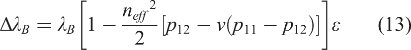
Simplifying the relationship by introducing a photoelastic coefficient, $p_e=\frac{{n_{eff}}^2}{2}\left[p_{12}-v\left(p_{11}-p_{12}\right)\right]$ yields the following relationship.

$\frac{\mathrm{\Delta }{\lambda }_B}{{\lambda }_B}=\left(1-p_e\right)·\epsilon \cong 0.78·\epsilon$

(14)

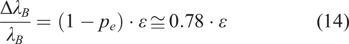
Researchers from China ⁵² investigated the feasibility of utilising fibre-bragg sensors for measuring NRT in rails. They utilised two fibre-bragg sensor constrained within the same optic-fibre cable, positioned 2 mm apart from each other, each with different cladding thickness for their study. The sensor cable was instrumented onto the rail web of a section of unspecified rail specimen with a cross-sectional area of 10.76 × 10⁻⁴ m ² and calibrations were carried out independently to determine the sensor’s sensitivity to temperature and strain. For the temperature calibration, the rail specimen was placed in a temperature-controlled enclosure and heated from ambient temperature at increments of 10°C from −30°C to +30°C. For strain calibration, the rail specimen was placed, under temperature-controlled conditions, in a loading machine and longitudinal compressive force was applied from 0.5 kN to 45 kN at 5 kN increments. The authors then constrained the rail specimen within the loading machine and heated the specimen up from −30°C to +30°C to impart thermal stress within the rail specimen. Their laboratory validation results show an accuracy similar to strain gauges, between 1.1 and 1.8°C. ⁵² As such, it is difficult to justify employing a strain gauge proxy that is considerably more expensive compared to conventional strain gauge with no additional benefits in terms of rail NRT measurement. The method would potentially have more merit used as a mass monitoring device for railway networks due to the ease of introducing Bragg gratings (measurement points) within a single optical cable.

Digital image correlation

Digital Image Correlation (DIC) was first conceived in the early 1980s ⁵³ by researchers from the University of South Carolina at the infancy of numerical computation and digital image processing. It utilises digital images of specimens under various loading conditions to deduce its strain and displacement fields. The images are typically captured sequentially, from a fixed charged-coupled device (CCD) camera typically mounted on a tripod, supplemented with lenses and lighting to maximize image contrast.^54,55 The number of camera used can be varied; a singular camera setup is called 2D-DIC whereas a twin camera setup is termed 3D or stereo-DIC. 2D-DIC operates on the assumption that deformations occurring within the sample are constrained within the plane parallel to the camera. As such, out-of-plane deformations will incur large errors in the strain and displacement fields. ⁵⁶ Stereo-DIC circumvents this by employing two or more cameras to generate 3D digital images of the specimen, enabling depth perception through triangulation at a higher monetary and computational cost.

Prior to any DIC measurements, surface preparation is required on the test specimen to produce a white speckle pattern. ⁵⁷ This is typically achieved by spray-painting the surface solid white then applying a thin mist of black paint. The resulting surface has a high-contrast and a non-uniform pattern, facilitating tracking of surface deformations across the captured images. For 3D-DIC, the measurement system consisting of cameras, lenses and lighting equipment is then installed and calibrated against a pattern consisting of black dots with known separation distance over a white background. ⁵⁸ This establishes the relationship between deformation in pixels and millimetre. For 2D-DIC, this can be done by taking a photo of an object (i.e., ruler) with a known length. After calibration, a series of images were taken as the specimen undergoes strain. The captured images are then subdivided into small square regions called subsets, each with unique gray level distribution. The transformation of these subsets across images was then computed mathematically with algorithms such as cross-correlation and sum of squared differences criterions. ⁵⁹ The resulting translation is converted from pixels into millimetres through the established calibration relationship to produce the specimen’s full-field strain measurement. The main advantage of DIC compared to conventional strain gauges lies in this capability of measuring the specimen’s 3D strain and deformation field rather than a single averaged point which a strain gauge provides.

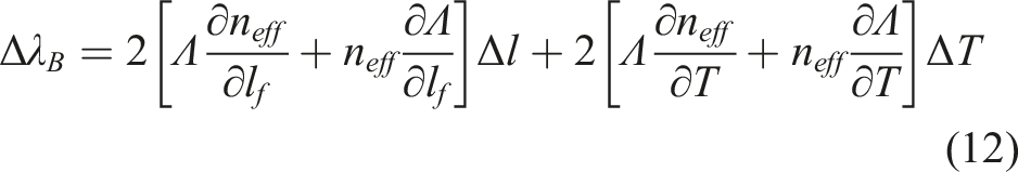
Recently, DIC has been trialled as a non-contacting method for determining NRT. ⁶⁰ Knopf’s DIC NRT measurement method ⁶⁰ summarised in Figure 6, relies on measuring web strain and rail head deformation at a region between two consecutive ties to estimate NRT and thermal rail stress. The authors theorised that due to the constraints typically imposed on railway tracks in the form of uniformly spaced fasteners and the longitudinal rail continuity, thermal expansion of rail will cause:

(a) non-uniform deformation of the rail head in the transverse plane

(b) variation in longitudinal and transverse stress, ${\sigma }_x$ and ${\sigma }_y$ at the web region located between two consecutive fasteners; maximum stress in the longitudinal direction, ${\sigma }_x$ with zero longitudinal strain, ${\epsilon }_x$ ( ${\sigma }_x\to {\sigma }_{\mathit{max}}$ , ${\epsilon }_x\approx 0$ ) and the opposite for transverse stress and strain ( ${\sigma }_y\approx 0$ , ${\epsilon }_y\to {\epsilon }_{\mathit{max}}$ ).

Figure 6.

Non-contacting DIC method for deducing NRT and thermal rail stress. ⁶⁰

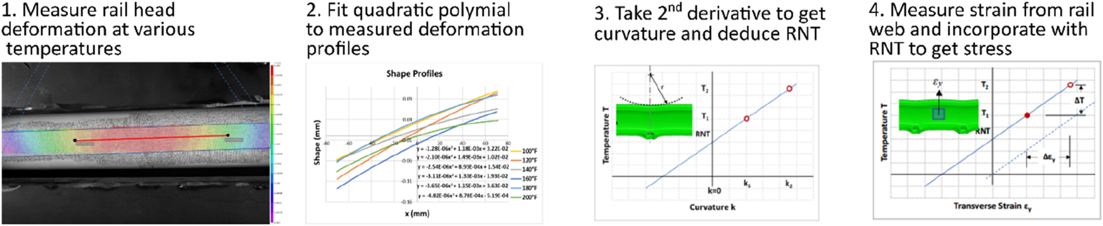
For their laboratory validation experiments, the authors measured the web strain, ${\epsilon }_x$ and ${\epsilon }_y$ and rail head deformation from a 16″ 132RE rail section, partially constrained longitudinally through welding two plates at both ends, at intervals of 11.11°C using a StereoDIC system. A quadratic polynomial was subsequently fitted onto the deformation profiles and the second derivative of the quadratic polynomial was taken to obtain curvature. The NRT was subsequently computed by calculating the y-intercept of the curvature-temperature relationship, which corresponds to the temperature at which the rail has zero curvature. As such this requires at least two measurement of rail head curvature at two different temperatures. The longitudinal rail stress, ${\sigma }_x$ was then computed using the transverse rail web strain, ${\epsilon }_y$ through the following equation where $E$ is the modulus of elasticity and $v$ is the Poisson’s ratio.

${\sigma }_x=\left(-{\epsilon }_y\right)\frac{E}{\left(1-v\right)}$

(15)

The authors achieved a NRT accuracy of between 2.7 and 4.4°C, ⁶⁰ demonstrating potential for a non-contacting NRT measurement solution. Despite this, the method has yet to be field validated and effects of different characteristics and types of rail fasteners, track stiffness, rail size and tie spacing on measurement accuracy have yet been investigated. The method also assumes that the rail head deformation at NRT is zero, which if it fails to hold, would require measurements at unstressed conditions that is reference. Despite claiming to be non-disruptive, the method would require a minimum of two measurements across a 11°C temperature change to achieve an accuracy demonstrated under laboratory conditions, which would only be feasible when measuring overnight and necessitates track closure for a single NRT measurement. In contrast, the industry standard, VERSE requires rail closure, but only for 2–3 hours. Apart from that, there is also the added complexity of surface preparation since DIC requires a speckle pattern to be applied onto the measurement zones and setup calibration.

Displacement methods

Displacement methods rely on measuring the change in distances between two positions to infer strain. The stress can then be computed through Hooke’s law. Solutions based on this is available commercially, with some products having more information in the public domain compared to others.

Pfender device

The Pfender device, ⁴ first introduced in Hungary, measures relative rail base elongation or shortening and converts the change in length into stress or NRT. For every 10 m of rail, pairs of balls were hammered into both sides of the rail web, separated by a distance of 100 mm. The distance between each pair of balls hammered into the surface is measured using a Pfender meter and the change in distance, $∆L_r$ is converted to stress, $∆\sigma$ via the following relationship.

$∆\sigma =E\frac{∆L_r}{L_r}$

(16)

The Pfender meter outputs both stress and strain information, with a NRT accuracy of 2°C. The device is prone to errors resulting from thermal expansion of components and thus is required to be calibrated regularly.

MS-02 device

The MS-02 longitudinal force gauge,^4,61 illustrated in Figure 7, is a device designed by Jacek Makowski for measurement of NRT. Weighing at a total of 1.55 kg, it measures the relative changes in the length of the gauge in relation to the measurement base under temperature fluctuations. This relative displacement is then converted into strain and subsequently longitudinal stress through Hooke’s law. Rail temperature is typically measured in addition to the relative displacement.

Figure 7.

The MS-02 measurement device (adapted from ⁶¹ ).

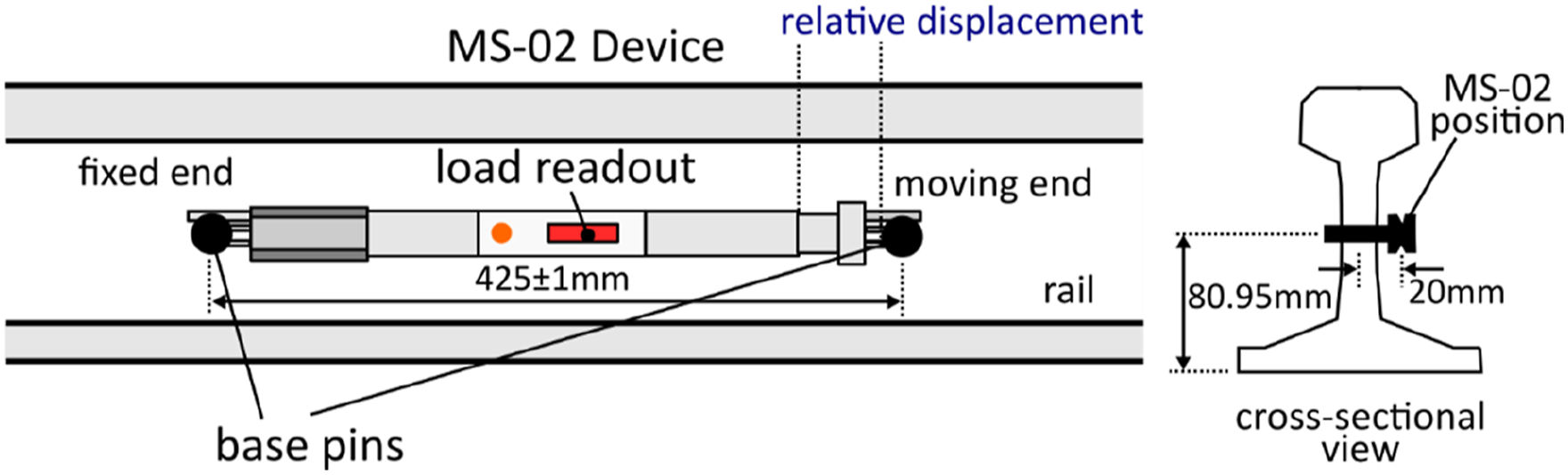
The gauge has a total length of 425 mm and consists of a casing, two pivots, one moveable whilst the other fixed to stabilise the position of the instrument relative to the pins during measurement and a digital display for direct reading of measurement. It is installed at the centre of the rail web where two 20 mm through holes are required for positioning the two pins. Alignment of the device relative to the longitudinal axis of the rail is crucial to avoid error. The method has a claimed accuracy of 5 kN or ±3°C ⁶¹ provided that the NRT is known at the time of installation.

Vibration

Resonance frequency method

A structure alters its modal characteristics (resonant frequency, mode shape) as its loading state changes. This is akin to a guitar string that changes its pitch when tightened. As such, changes in resonant frequencies of a structure can be used to infer its loading state.

This method was pioneered for rail stress measurement in 1979 by researchers from Foster-Miller Associates ⁶² who analytically and experimentally quantified the change in flexural vibration frequencies of a finite length of rail with varying compressive loading, for a frequency range between 1 and 10 kHz. Through their laboratory investigations, they observed a shift in resonant frequency with compressive stress however acknowledged that changes in rail end conditions will significantly influence the measurement. Researchers from Association of American Railroads ⁶³ furthered the investigation by testing on two 12 m long 136RE test rail, laid on ties set in crushed limestone ballast. The rails were instrumented with strain gauges to monitor compressive loading delivered by rail pullers at four loading intervals: 3.5, 20.7, 35 and 48 MPa. Impact excitation was applied to the rail web at each loading intervals and acoustic vibration was measured through a microphone positioned at right angle to the rail web. The resonant frequency varied from 1 to 5 kHz as the compressional force increased from 3.5 to 48 MPa. The research, despite addressing challenges pertaining to on-site testing, also did not address the influence of tie-to-tie variations on measurement accuracy.

To resolve this issue, researchers from Virginia Polytechnic Institute ⁶⁴ developed analytical models which established the theoretical relationship between resonant frequencies, axial forces, and support stiffness. The theoretical investigation extended into the first eight modes of resonances and quantified the sensitivity of each resonance mode to support stiffness and axial loading. Through measuring the frequency of resonance vibration, the possible combinations of support stiffness and axial loads can be computed for each resonance mode. The intersection point of all the resonance modes yields the estimated support stiffness and axial loading.

Experimental validation tests were conducted on a 5-m I-beam where it was loaded from 15 to 76 MPa at 15 MPa increments. The mode shape and natural frequencies of the beam was determined through calculating the response amplitude and phase for a series of excitations along the beam. Experimental results revealed an accuracy of ±41.5 MPa or ±17.4°C with the error attributed to uncertainty in lateral stiffness of the end supports. This demonstrates the primary limitation of the method as well as the challenges in accurately modelling end supports.

Livingston et al. ⁶⁵ devised a similar method as Boggs ⁶⁴ for estimating the support stiffness and axial loading through resonant vibrations signals. They measured the resonant frequencies of a square steel rod under tension up to 58 MPa and noted a linear relationship between the resonant frequencies and tensile load and attained a max error of ±7.396 MPa or ±3.2°C. However, dependency on boundary conditions that is the rail fixings onto sleepers still affects measurement accuracy.

More recently, efforts have been made to develop a contactless, video-based approach for measuring rail head vibration to infer NRT. ⁶⁶ The method utilizes a high-speed camera to record rail head vibrations as the rail is excited with an instrumented hammer. Modal characteristics (resonant frequency and mode shapes) of the rail were extracted from each pixel within the video image as they act as virtual accelerometers. The axial stress is subsequently inferred through the extracted modal characteristics. Laboratory validation tests were performed on a 2.4 m long 132RE rail, constrained axially by a hydraulic press. The test specimen was adequately illuminated through four studio lights whilst video measurements of the specimen was taken with a white background. To improve image contrast, “QR code” printouts were attached to the rail head surface. Accelerometers and strain gauges were also instrumented onto the rail. The rail was compressed in 12.05 MPa increments up to 96.39 MPa with measurements captured at each load increment. Through extracting the displacements at the pixels adjacent to the “QR code” printout, the rail resonances were successfully identified. The identified resonance frequencies agreed well with those identified from the accelerometer measurements, demonstrating the capability of the non-contacting system to replicate measurements from the contacting accelerometer bonded onto the rail. No accuracy is quoted, however if the method produces measurements akin to bonded accelerometers, accuracy will mirror the bonded instrumentation setup. The method, however, still needs to overcome challenges associated with field deployment which include illumination and high contrast issues from the sun and rail surface with varying wear condition, as well as the influence of residual stresses and rail fasteners on the measurement accuracy.

According to Ref. 4, a commercial product based on the vibration method does exist under the trade name Rail Vibrating Wire (RAFT). It was supposedly used by British Railways, which ceased operation in 1997. Instead of vibrating the rail, a wire is installed along the rail and excited to measure relative force change in the rail.

Vibration – D’stresen

A variant of the vibration method is the use of vibrational torsional rigidity to infer NRT. ⁶⁷ This has been commercially marketed in 2008 as D’stresen ⁶⁸ by Jury & Jury Technologies based in New Zealand. The method exploits the change in rail lateral and torsional stiffness with thermal stress, which in turn varies the resistance of rail against forced rotational motion introduced by an external force such as a shaker. The rail vibration amplitude varies proportionally with the rail axial thermal loading, as illustrated in Figure 8(a). Since the rail has the least resistance at zero thermal stress, the amplitude of vibration peaks at the NRT. Thus, the NRT can be estimated through monitoring the temperature and vibrational response of rail. Note that the relationship gradient varies for rails in tension and compression.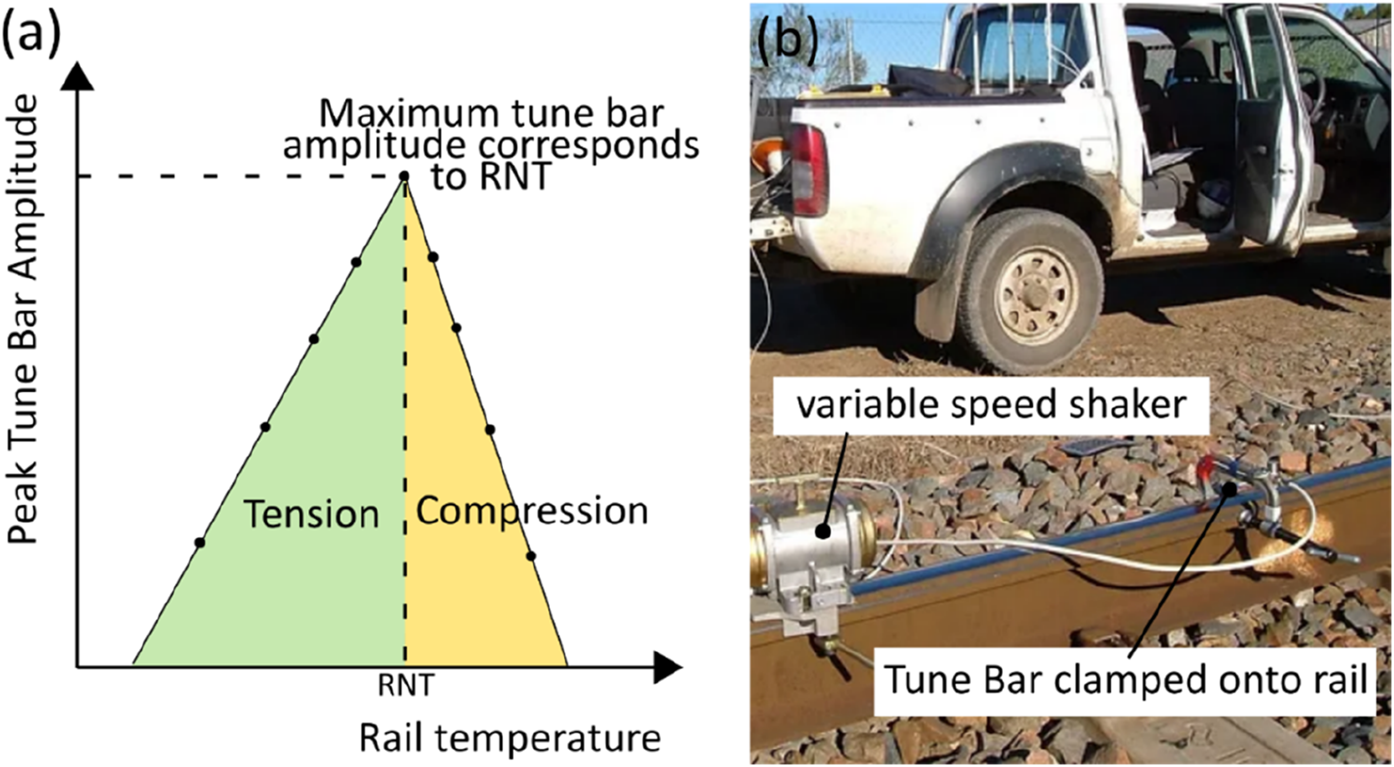

Figure 8.

(a) Relationship between peak TB amplitude and rail temperature ⁶⁷ and the D’Stresen system in operation. ⁶⁸

The D’stresen system, as shown in Figure 8(b) consists of a shaker, tuner bars, data acquisition unit, temperature probe and a computer. The shaker and twin tune bars are clamped onto the rail head. The shaker delivers low frequency excitation (65–80 Hz) and displacement of up to 0.2 mm to the rail head. Accelerometers mounted at the end of each tune bars measure the rail’s first bending resonance and the vibration data alongside rail temperature is then transmitted to the computer and processed for the peak vibration amplitude corresponding to the NRT. Accuracy of the D’stresen method is quoted at ±8.3°C or 19.76 MPa when compared with VERSE and strain gauge data. ⁶⁷ The approach, contrary to VERSE, does not require unfastening of rails. However, the method, similar to the resonance frequency method, is sensitive to rail fastening and support conditions. Measurements are also restricted to when the rail is in tension. There is also the lack of experimental evidence to validate the relationship between tune bar vibration amplitude and rail temperature. ⁶⁹

Guided wave technique

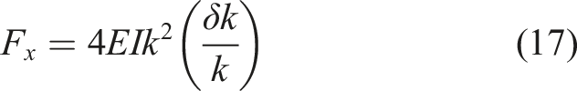
Researchers from University of Illinois^70,71 proposed a variation which circumvents the boundary condition dependency. The proposed method utilizes the lateral bending wavenumber, 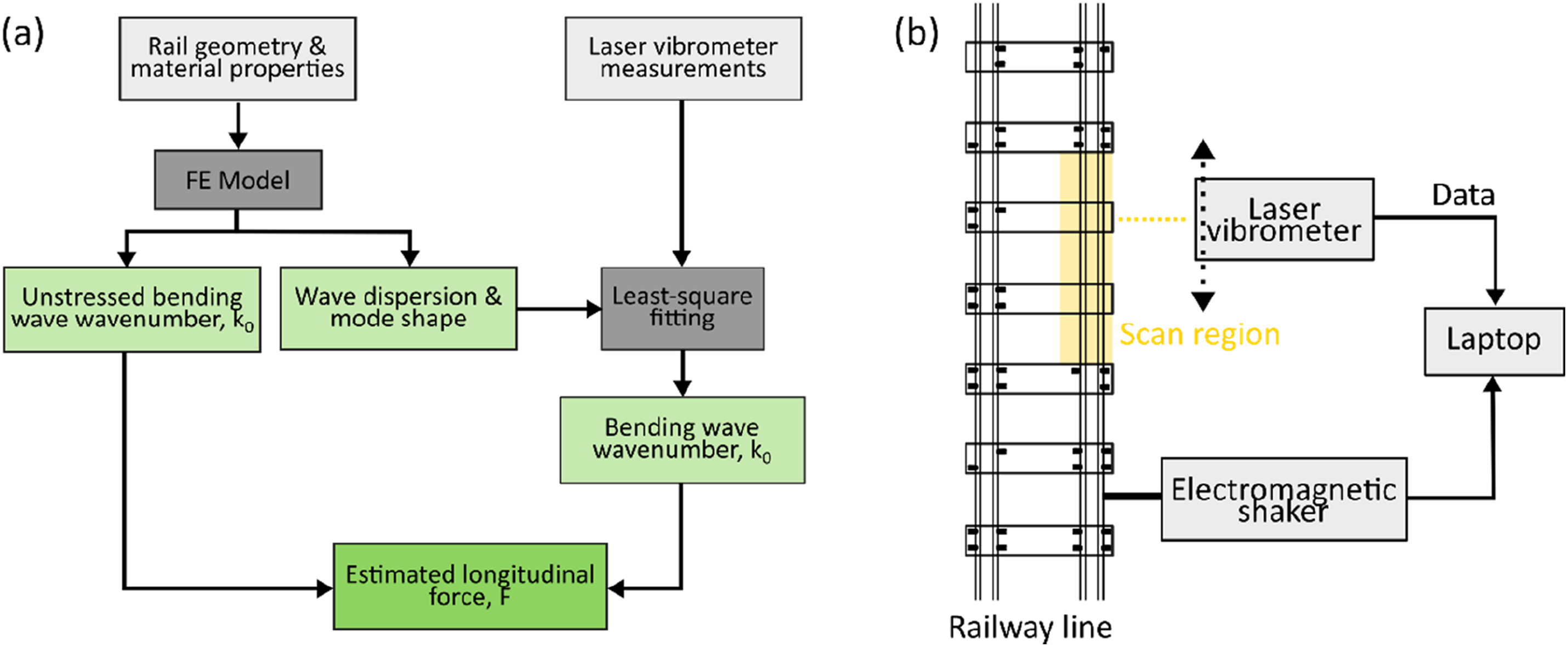$k$ instead of the resonant frequency of rail under thermal stress, to infer the longitudinal force, $F_x$ in rail. This guided wave technique is based on the Euler-Bernoulli beam theory which simplifies down to the following relationship.

$F_x=4EI{k}^2\left(\frac{\delta k}{k}\right)$

(17)

$E$ is the modulus of elasticity, $I$ is the second moment of area and $k$ is the lateral bending wavenumber, and $\frac{\delta k}{k}$ is the best-fit amount of distortion of $k$ , obtained from fitting the measured displacement profile to theoretically expected guide modes and wavenumbers, determined by high-precision Finite Element (FE) Modelling. Theoretically, the relationship intercepts at zero and behaves linearly for 136RE rails under 51.74 MPa. The framework for the guided-wave technique is summarised in Figure 9(a). By inputting precise rail geometry and material properties into wave dispersion models,^72,73 the reference wavenumber at zero-stress, $k_0$ as well as the wave dispersion mode shapes can be obtained. The latter information is then used to decouple desired vibration modes (lateral flexural mode) from vibration data obtained by the non-contacting laser vibrometer. The extracted wavenumber alongside the reference wavenumber is then used to estimate the longitudinal force using equation (17).

Figure 9.

(a) Methodology and (b) test setup for the vibration based guided-wave technique for estimating longitudinal forces in rail using wavenumber.^70,71

A schematic of the experimental setup is shown in Figure 9(b). An electromagnetic shaker delivers excitation at specific frequencies to the rail structure. A small section of rail is unclipped (1.4 to 2 m) and non-contacting vibration measurements are captured across the unsupported span using a laser vibrometer.

Initial validation tests were conducted on a 2.33 m long 136RE rail section. The rail section was loaded axially in compression with a hydraulic actuator and vibrated at its corresponding resonant frequency to ensure the strongest dynamic response. About 1.4 m of rail was unclipped and two longitudinal scans along different points on the rail cross-section were taken using a laser vibrometer and an accelerometer which acted as a reference. Post-processing involved a “lock-in” process which improved signal-to-noise ratio. The measured displacement profile was then fitted to theoretical expectations using non-linear least square fitting and a linear relationship between longitudinal load, $F$ and best-fit distortion amount of $k$ , $\frac{\delta k}{k}$ was established. Despite this, an offset was observed at zero-stress which incurred an error of 17.79 MPa or 7.47°C.^70,71 The error was attributed to inaccuracies in the cross-sectional area of rail steel used for the FE analysis, demonstrating the methods’ sensitivity to rail geometry.

Subsequent blind tests ²⁹ performed on 136RE rails with varying degree of wear, where the compressive loads were not disclosed to the operator, yielded an accuracy of ±13.98 MPa/±5.87°C for unworn rail and ±33.14 MPa/±13.92°C for the worn 136RE rail. The accuracy was compromised due to the lack in understanding of complex bending and torsional waves in worn rails and presence of measurement drift which was largely circumvented through the use of multiple reference accelerometers positioned on the rail.

Kjell and Johnson ⁷⁴ carried out an independent study on the guided wave technique using a setup which mimics an actual railway system. Their experiment used two 11 m 60E1 rails fixed to sleepers and pads. One of the rails was fixed at one end and loaded at the opposite end. In the rail’s middle section, where accelerometer readings were taken, three sleepers were left unclamped, and an excitation of around 330 Hz was introduced using a shaker. Instead of using a non-contacting laser vibrometer setup, rail longitudinal deflection was measured using conventional accelerometers bonded at different points on the rail. The wavenumber was subsequently determined through a least square fitting routine and compared with the reference wavenumber to yield longitudinal force. Although achieving better precision at ±4°C, zero-offset problems persisted. Kjell and Johnson ⁷⁴ highlighted several challenges with the technique, such as the sensors’ sensitivity to temperature and placement, dependence of friction between the rail and pads in loosened clamps, lengthy FE computation time due to requirements for fine mesh, and the need for precise rail geometry, wave speed in rail, and Poisson ratio for accurate measurements.

Electro-mechanical impedance (EMI)

The EMI method^75,76 involves measuring changes in the electrical admittance signature of a piezoelectric element bonded onto the rail to estimate the longitudinal stress and subsequently calculate the NRT. The element is typically made of lead zirconate titanite (PZT). As the rail is stressed, the strain is transferred to the PZT through the adhesive layer. This alters the properties (piezoelectric constants and dielectric permittivity) of the PZT ⁷⁶ which manifests itself as variation in electrical admittance.

To validate the method, researchers from University of California ⁷⁶ carried out laboratory tests on both aluminium and steel specimens. The steel specimen comprised of a web section machined out of a 136RE rail. Prior to testing, both specimens were instrumented with a PZT element, bonded with strain gauge adhesive and strain gauges. The aluminium specimen was loaded within a hydraulic machine from +34.47 MPa (tensile) to −34.47 MPa (compression) at measurement intervals of 6.89 MPa. The loading range was 4-fold higher for the steel specimen, with a measurement interval of 34.47 MPa. Electrical admittance was obtained from each load interval and subsequently, 3 parameters were identified to vary linearly with axial stress. These were shifts in the conductance resonance peaks, electrical resonance peaks and the capacitance of the PZT element. Among the 3 parameters, the capacitance was found to be most sensitive to stress variation at 0.96 pF/MPa. ⁷⁶

Provided that a zero-stress reference is available, based on the results presented in Ref. 76, the EMI method can achieve a ±2.5°C NRT accuracy. However, such a reference is often not available in modern railway tracks. The method however could still be used as a long term NRT monitoring solution in which piezo elements are installed alongside fresh railway tracks and its variation in admittance measured and converted to axial loading. For the method to be sufficiently robust for track implementation, effects of hysteresis during cyclical loading on the reversibility of admittance and temperature variation on the accuracy of the axial load estimation needs to be studied. Apart from that, the influence of varying bond layer on the measurement accuracy also needs consideration as surfaces of rail in operation will vary in degree of wear and rust, subsequently affecting the uniformity of bond layer.

Ultrasound

Acoustic waves are mechanical disturbances occurring within a medium due to energy transfer across the particles within the medium. Ultrasonic waves specifically refer to acoustic waves operating beyond the audible range of human hearing (>20 kHz). The propagation speed of ultrasonic waves within a material is dependent on its stress state. This variation is termed the acousto-elastic effect and depends on the polarisation (direction of particle displacement) and propagation direction of the ultrasonic waves relative to the stress field.

Equations governing these are first published by Hughes and Kelly ⁷⁷ and later adopted by Egle and Bray ⁷⁸ for rail thermal stress measurement. Considering a state of uniaxial stress acting in the $1$ -direction, the relationship between ultrasonic propagation speeds, $V_{ij}$ and strain, $\epsilon$ can be mathematically described as shown below, ⁷⁸ where ${\rho }_0$ is the unstressed density, $v$ is the Poisson ratio, $V_{ij}$ is the speed of sound propagating in the $i$ -direction, polarised in the $j$ -direction, $\lambda$ and $\mu$ are second-order elastic constants, and $l$ , $m$ , $n$ are third-order elastic constants.

${\rho }_0{V}_{11}^2=\lambda +2\mu +\left[4\left(\lambda +2\mu \right)+2\left(\mu +2m\right)+v\mu \left(1+\frac{2l}{\lambda }\right)\right]\epsilon$

(18)

${\rho }_0{V}_{12}^2={\rho }_0{V}_{13}^2=\mu +\left[4\mu +v\left(n/2\right)+m\left(1-2v\right)\right]\epsilon$

(19)

For ultrasonic waves travelling perpendicular to the uniaxial stress, that is sending sound waves perpendicular to the longitudinal rail length,

${\rho }_0{V}_{22}^2=\lambda +2\mu +\left[2l\left(1-2v\right)-4v\left(m+\lambda +2\mu \right)\right]\epsilon$

(20)

${\rho }_0{V}_{21}^2={\rho }_0{V}_{31}^2=\mu +\left[\left(\lambda +2\mu +m\right)\left(1-2v\right)+0.5nv\right]\epsilon$

(21)

${\rho }_0{V}_{23}^2={\rho }_0{V}_{32}^2=\mu +\left[\left(\lambda +m\right)\left(1-2v\right)-6v\mu -0.5n\right]\epsilon$

(22)

The level of sensitivity of ultrasonic waves to stress can be further derived from these equations. These are presented as relative changes in wave speed with axial strain, $L_{ij}=\frac{d{V}_{ij}/V_{ij}^0}{d\epsilon }$ where $d{V}_{ij}$ is the change in wave speed, $V_{ij}^0$ is the unstressed speed of sound and $d\epsilon$ is the change in strain. Table 1 shows the sensitivity of ultrasonic waves with varying polarisation and propagation to uniaxial stress in the $1$ -direction. A negative value indicates that the relative change in sound speed decreases with increasing strain and vice versa. Conversely, a larger magnitude represents larger change in sound speed with strain, indicating higher sensitivity. From Table 1, the longitudinal wave propagating in the longitudinal direction (parallel to the axial stress), $L_{11}$ has the highest sensitivity, followed by shear waves propagating perpendicular to the axial stress but polarised in line with the axial stress, $L_{21}$ . Table 2 shows the second and third order elastic constants for US rail steel from Egle & Bray. ⁷⁸

Table 1.

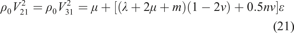
Sensitivity of ultrasonic waves to uniaxial stress.

	Sensitivity parameter	Value 78
$L_{11}$	$2+\left[\mu +2m+v\mu \left(1+\frac{2l}{\lambda }\right)\right]{\left[\lambda +2\mu \right]}^{-1}$	$-2.43\pm 0.05$
$L_{12}$	$2+0.25vn{\mu }^{-1}+0.5m{\left(\lambda +\mu \right)}^{-1}$	$0.01\pm 0.1$
$L_{22}$	$-2v\left[1+\left(m-\mu l/\lambda \right){\left(\lambda +2\mu \right)}^{-1}\right]$	$0.27\pm 0.01$
$L_{21}$	$0.5\left(\lambda +2\mu +m\right){\left(\lambda +\mu \right)}^{-1}+0.25vn{\mu }^{-1}$	$-1.51\pm 0.02$
$L_{23}$	$0.5\left(m-2\lambda \right){\left(\lambda +\mu \right)}^{-1}-0.25n{\mu }^{-1}$	$-0.27\pm 0.12$

Table 2.

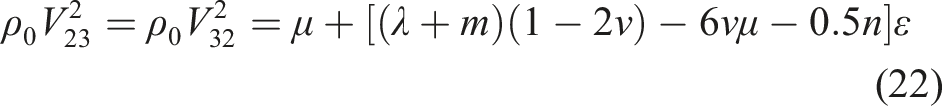
Second and third order elastic constants for rail steel. ⁷⁸

Parameter	${\rho }_0$ $\left(kg/m^3\right)$	$\lambda$ $\left({10}^{10}\hspace{0.17em}N/m^2\right)$	$\mu$ $\left({10}^{10}\hspace{0.17em}N/m^2\right)$	$l$ $\left({10}^{10}\hspace{0.17em}N/m^2\right)$	$m$ $\left({10}^{10}\hspace{0.17em}N/m^2\right)$	$n$ $\left({10}^{10}\hspace{0.17em}N/m^2\right)$
US rail steel	$7799.5\pm 0.5$	$11.33\pm 0.26$	$8.12\pm 0.13$	$-27.5\pm 2.7$	$61.95\pm 0.35$	$71.9\pm 0.5$

Table 3 summarises the different variants of ultrasonic setup used by researchers in attempt to measure NRT. All attempts except for Nucera et al. ⁷⁹ operate through the principle of acousto-elasticity, with differences either in the type of waves used or the direction of wave propagation relative to the longitudinal rail thermal stress.

Table 3.

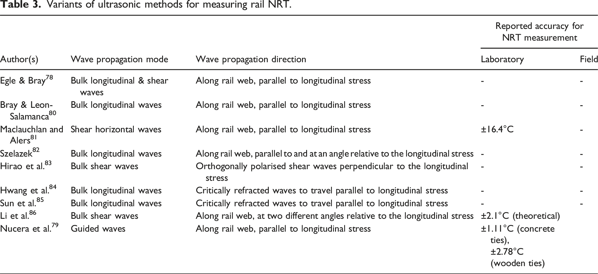
Variants of ultrasonic methods for measuring rail NRT.

Author(s)	Wave propagation mode	Wave propagation direction	Reported accuracy for NRT measurement
			Laboratory	Field
Egle & Bray 78	Bulk longitudinal & shear waves	Along rail web, parallel to longitudinal stress	-	-
Bray & Leon-Salamanca 80	Bulk longitudinal waves	Along rail web, parallel to longitudinal stress	-	-
Maclauchlan and Alers 81	Shear horizontal waves	Along rail web, parallel to longitudinal stress	±16.4°C	-
Szelazek 82	Bulk longitudinal waves	Along rail web, parallel to and at an angle relative to the longitudinal stress	-	-
Hirao et al. 83	Bulk shear waves	Orthogonally polarised shear waves perpendicular to the longitudinal stress	-	-
Hwang et al. 84	Bulk longitudinal waves	Critically refracted waves to travel parallel to longitudinal stress	-	-
Sun et al. 85	Bulk longitudinal waves	Critically refracted waves to travel parallel to longitudinal stress	-	-
Li et al. 86	Bulk shear waves	Along rail web, at two different angles relative to the longitudinal stress	±2.1°C (theoretical)
Nucera et al. 79	Guided waves	Along rail web, parallel to longitudinal stress	±1.11°C (concrete ties), ±2.78°C (wooden ties)

Non-linearity in bulk longitudinal and shear waves (acousto-elasticity)

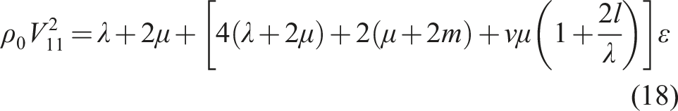
Egle and Bray ⁷⁸ pioneered the development of an ultrasonic-based method for longitudinal stress measurement in rail. They were first to quantify the third-order elastic constants of US rail steel (Table 2). Laboratory tests were conducted on three rail specimens from various parts of the rail, manufactured at different years to cover various heat treatments and rail composition. To pulse ultrasonic waves longitudinally along the rail, longitudinal and shear sensors are mounted on plexiglass wedges and critically refracted at 28° for longitudinal and 55° for shear. The transducer bonding method (permanent cement or viscous resin with spring loading) was found to have little effect on the ultrasonic wave speeds. They also concluded that the longitudinal wave propagating parallel to the applied stress is most sensitive to stress as and found that the acoustoelastic constants are relatively independent of specific composition and heat treatment.

The time-of-arrival (ToF) of ultrasonic waves are used to obtain ultrasonic wave speeds. The travel path, L is usually known or measured. Typical values for longitudinal waves in rail is 5945 m/s, nearly twice the speed of shear waves at 3226 m/s.

Bray and Leon-Salamanca ⁸⁰ used longitudinal subsurface waves to measure thermal rail stress. The ultrasonic waves were sent along the rail web and ToF of the ultrasonic pulses were measured. The authors proposed averaging measurements from several rail specimens to eliminate the influence of residual stresses and rail texture.

Maclauchlan and Alers ⁸¹ utilised surface skimming shear horizontal ultrasonic waves generated by EMATs for measurement of rail stress. Ultrasonic waves of 2 MHz are generated in a rail sample, which was then subjected up to 103.4 MPa of tensile and compressive loading. A linear relationship was obtained between the transit time difference and applied loading; however, a 38% difference/error (39 MPa or ±16.4°C) was observed between the measured and theoretical transit times.

Szelazek ⁸² exploited the sensitivity of longitudinal waves propagating in the stress direction ( $L_{11}$ ) to infer thermal stresses in rail. The designed ultrasonic probe-head, attached onto the rail head, consists of one transmitter and two receiver probes of 2 MHz frequency.

The system generates longitudinal waves in two direction: parallel and at an angle relative to the longitudinal stress. The latter travels through the rail head at an angle and is reflected as it strikes the opposite edge of the rail head. The reflected waves are subsequently captured by one of the receiver probes and sampled at a 1 GS/s using the DEBRO-30 device.

Laboratory tests involved quantifying measurement scatter through varying the probe’s position in the lateral and transverse direction. Measurements were found to vary as the probe is moved vertically upwards to the rail head due to the change in residual stress, however little variation is observed when the probe is shifted laterally. The latter measurements were also repeated during track trials on 49E1 rails. A scatter of 21 ns was found for the subsurface waves whereas 42 ns scatter was attributed to the reflected waves. Szelazek noted that the factors affecting repeatability of ToF measurements include residual stresses in rail, material texture and interface of the sensor (roughness of rail). Since the former two varies insignificantly across the scanned distance, the scatter observed is likely due to differences in acoustic coupling from variation in roughness of the rail surface. This constitutes between 70 and 140% of error as the time-of-flight change measured ranges between ±30 ns.

Track trials were conducted on a newly laid railway line. Prior to opening of the track, time-of-flight measurements were taken across a 400 m unclipped rail section. These measurements are free of thermal and operational residual stresses and thus serve as reference. Measurements were subsequently taken after 10 months of operation across the same section. A change in time-of-flight was observed between the two datasets; however, since measurements are taken blind, it is not possible to discern the accuracy of the method. The change observed will also be comprised of residual stress variation between freshly laid tracks and after 10 months of operation. Szelazek’s method can potentially be used qualitatively, however for absolute stress values, more refinements are necessary.

In 1994, researchers from Japan ⁸³ were first to propose the use of acoustic birefringence for measurement of thermal rail stress. They used non-contacting EMAT sensors to generate orthogonally polarised shear waves on sections of rail. Laboratory testing involved compressing Shinkansen rail sections (JIS-60) of 0.5 m long up to 76 MPa. Two methods were used; pulsed resonance spectroscopy applied on the rail web and phase shift method applied from the rail head through the foot. A major source of error was due to positioning of EMATs as they rotate the sensor from 0 to 90° to generate the shear waves.

Compressive residual stresses were also measured, around 150 MPa for the rail web. Pulsing from top-to-bottom smoothens the local texture and residual stress variation and subsequently residual stresses tend to zero. Liftoff errors were found to be as high as 24 MPa when gap is >1 mm which is very likely when testing in field. Authors note that this also includes position uncertainty error, thus liftoff error would be lower than reported. Authors also noted that temperature affects the texture offset parameter weakly (50°C gives an error of 2.5 MPa), but also noted that temperature would affect the acoustoelastic constants. No estimates were given. They proposed that the ultrasonic response consists of the acoustoelastic parameter as well as an offset resulting from texture anisotropy.

Researchers from Korea ⁸⁴ proposed a method using longitudinal critically refracted waves for thermal and residual stress measurement. Longitudinal waves are sent at the critically refracted angle from a less dense material (PMMA) into the rail steel and due to Snell’s law, the wave is refracted and propagates along the length of the rail steel. The method exploits the sensitivity of bulk longitudinal waves propagating in line with the applied stress ( $L_{11}$ ). They fabricated a sensor wedge made out of PMMA using 2.25 MHz piezo elements. The sensor wedge consists of 3 sensors: 1 transmitter and 2 receivers. Laboratory tests conducted on specimens machined out of two used KR60 rail sections and loaded in tensile up to 374 MPa yielded linear relationships between change in time-of-flight and stress. The extracted acoustoelastic constants, $L_{11}$ (−2.798 & −2.823) were very similar to that reported in Ref. 80. The authors also measured the variation in residual stresses across the rail head from 3 rail sections. Through analysing the patterns of residual stress across the rail head, they were able to deduce the origin of the rail section; straight tracks where residual stress distribution is more uniform or curved section with higher residual stress at the rail edge where higher contact occurs. Such measurements are difficult to be translated onto track due to influence of thermal stresses and as such has little value outside laboratory conditions.

Researchers from China ⁸⁵ implemented the longitudinal critically refracted method on the Shanghai-Nanjing high speed railway track in China. They designed PMMA wedges instrumented with 5 MHz ultrasonic sensors to send longitudinal critically refracted waves. They also designed an online monitoring system which consists of thermocouple, ultrasonic sensors, 4G wireless communication module, powered by a battery. They provided material properties for 60 kg rails and quoted an acoustoelastic constant at −2.51. They also showed a calibration curve for 60 kg rails, a linear relationship exists between the stress and ToF but it isn’t clear how the calibration curve is obtained. Trends between rail temperature and ultrasonic ToF were obtained, they correlate proportionally. However, effects of temperature on ultrasonic wave speed were not eliminated. Also, since the residual stress is not quantified, it is unclear how the data can be translated to NRT.

Recently, Li et al. ⁸⁶ proposed a new method of measuring rail stress. The method relies on sending two shear waves at two different angles, ${\theta }_1$ and ${\theta }_2$ across the rail thickness to deduce the stress state of rail. The sum of angles ${\theta }_1$ and ${\theta }_2$ needs to be 90°. The difference is propagation speeds between the two shear waves is proportional to the stress and independent of material properties. As such the method warrants no calibration. A virtual FE experiment was conducted by the authors to validate their method. The error incurred was <1% for applied stress lower than 500 MPa. Assuming a 1% error at 500 MPa, this translates to an error of ±2.1°C. The method shows promise for rail thermal stress measurement; however, it would potentially be difficult to implement due to the level of setup precision necessary to maintain errors under acceptable conditions.

Non-linearity in ultrasonic guided waves

Nucera et al.^79,87 proposed a method based on non-linear ultrasonic guided waves for NRT measurement. The method relies on measuring non-linearities arising in waveguides travelling in rails. Due to boundary restrictions, thermal energy introduced into the rail is instead converted into potential/vibrational energy. This alters the interatomic potential state of the rail and subsequently the average bonding distance between atomic particles, incurring higher-order, non-linear harmonics in the ultrasonic guided waves. ⁸⁷

Simulations were initially carried out using a proprietary non-linear finite element (SAFE) algorithm to select the mode of ultrasonic guided waves for propagation in the webs of 136RE rails. The simulated results, as illustrated in Figure 10(a), include wavenumber and phase velocities for guided waves up to 600 kHz. Subsequently, a frequency of 200 kHz was selected as it promotes flexural horizontal modes propagating in the rail web. Laboratory validation trials follow after and were conducted at University of California San Diego’s large scale test bed on 21 m long rails. The rails were subjected to heating and cooling cycles up to 65.56°C. Instrumentation include temperature compensated strain gauges, thermocouples, and infrared camera. A measurement device called “Rail-NT” was built to generate and receive guided waves. The device consists of an ultrasonic transmitter and receiver which operated in pitch-catch mode with magnets to mount onto the rail web. The measured non-linear parameter, β varies proportionally with rail temperature, with inflection points (minima) corresponding to the NRT, visible in Figure 10(b). An accuracy of ±1.11°C was successfully achieved in the laboratory.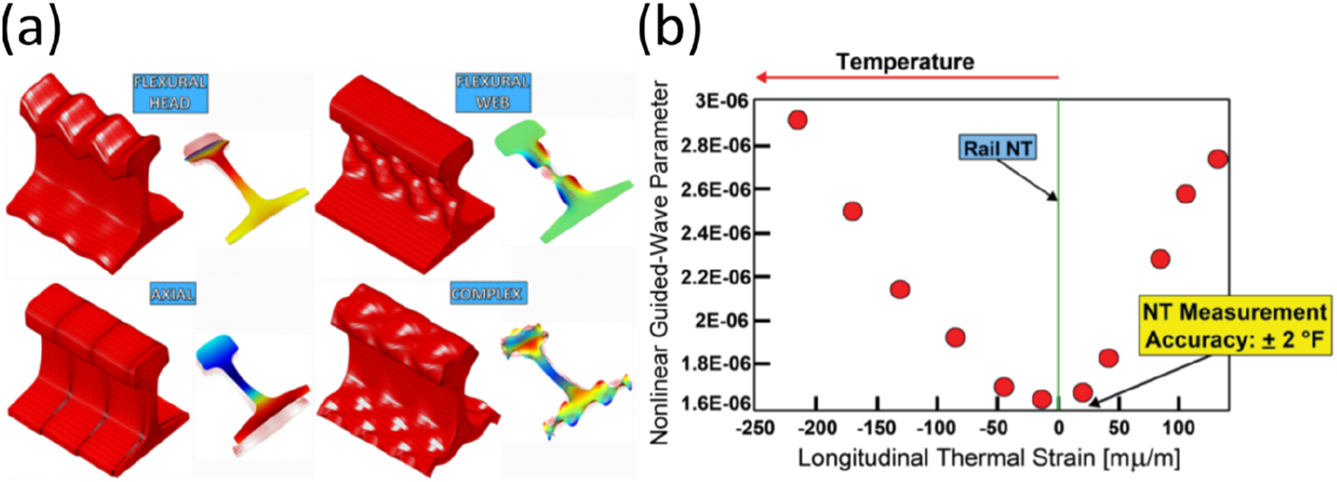

Figure 10.

(a) Various propagation modes computed from the finite element model ⁸⁷ and (b) relationship of nonlinear guided-wave parameter, β with longitudinal thermal strain: minima corresponding to the rail neutral temperature. ⁷⁹

Field trials carried out in Transportation Technology Center (TTC) in Pueblo, Colorado on 141RE rails with a transition between wooden and concrete ties yielded an accuracy similar to laboratory testing for concrete ties (±1.11°C) and slightly higher errors for wooden ties (±2.78°C). In addition to the good accuracy, the measurement system is also non-disruptive to normal service. The mounting system, however, requires a redesign as it failed to prevent sensor misalignment due to a passing train. ⁸³ The main limitation of the system lies in the need for the rail temperature to intersect NRT during the measurement period. Practically, this could mean lengthy measurement periods. Additionally, the method’s accuracy on other types of railroad ties (steel, plastic composite) warrants further investigation.

Magnetic Barkhausen Noise (MBN)

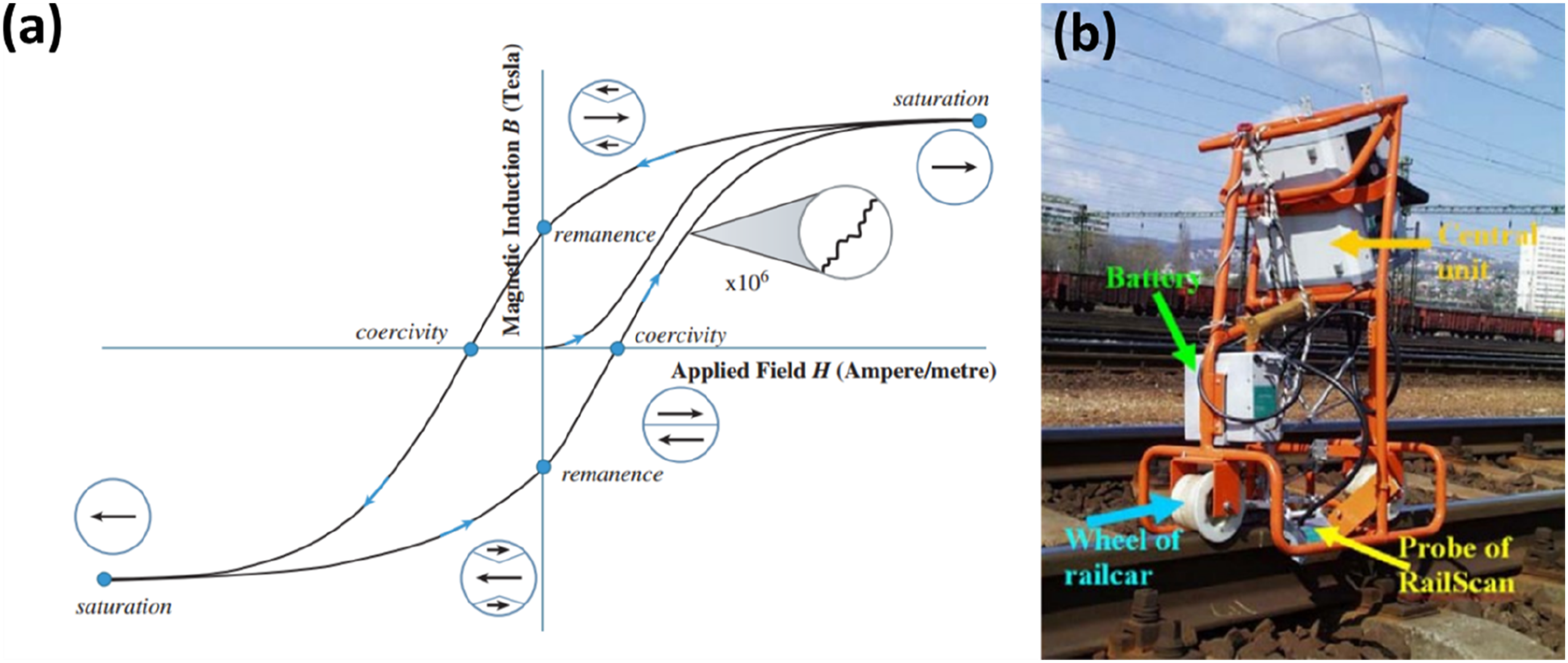
Ferromagnetic materials are made of micro magnetic domains, which is a region of uniform magnetisation. The direction of magnetisation differs from one domain to the next, and so there is a net zero magnetisation across the entire specimen, despite these domains being magnetically saturated on a micro scale. When a magnetic field is applied to a ferromagnetic material the magnetic domains are aligned, giving the part magnetic anisotropy in the direction of the applied field. During this realignment there is localised domain movement due to the magneto-elastic effect. When the field is removed, there is a relaxation of domains back to the equilibrium position; this relaxation can be visualised in Figure 11(a) with the observable hysteresis behaviour. However, the line is not smooth, and irregularities occur due to localised magnetic domains. ⁸⁸

Figure 11.

(a) Magnetic induction hysteresis with cyclic application and 180° reversal of applied field ⁸⁸ (b) RailScan system fitted onto track. ⁵

When the applied field moves through the zero position the magnetic domain (MD) attempt to return to their original alignments. Pinning sites refer to material grain boundaries, dislocations, inclusions, and any other physical feature that can restrict movement and slow down MD movement. Energy is needed to overcome pinning sites; this energy use is observed as small step changes in magnetism which in turn give electrical current variations, referred to as Magnetic Barkhausen Noise (MBN). ⁸⁸

Stefanita et al. ⁸⁹ studied the sensitivity of the MBN method on elastically and plastically deformed samples. They found that within the elastic region, tensile stress increases MBN energy and creates a magnetic easy axis in the stress direction through reorientation of domain walls. This is an opposite effect to compressive stress, which reduces MBN energy and therefore creates a magnetic easy axis perpendicular to the direction of stress. ⁹⁰ In the plastic region the MBN energy is affected by an increased number of pinning sites, rotation of the easy axis due to texture change and localised stress increases related to work hardening. ⁸⁹ However, these changes of magnetism are small compared with the initial alignment of the easy axis within the elastic region, meaning the MBN method is far more sensitive within the elastic region when compared with the plastic region.

Wang et al. ⁹¹ used MBN sensors and a root-mean-square (RMS) analysis technique to measure stress and found a linear relationship within the elastic region, and a less sensitive monotonic relationship in the plastic region. The work was expanded on in Ref. 92 showing there are several ways to interpret MBN signals with differing levels of accuracy, with the potential to combine methods in future to reduce errors even further.

Santa-aho et al. ⁹³ reviewed MBN methods for CWR stress measurements, and highlighted RailScan, ⁹⁴ a commercial device using the MBN method to measure stress in CWR. Figure 11(b) shows the RailScan system fitted onto track ⁵ . For the device to work, calibration with a rail specific specimen of similar condition to the in-field rail under compressive, tensile and no load is required.^5,93,95

Zhang ⁹⁵ compared RailScan measurements with installed strain gauges and Verse NRT measurement methods, with a NRT difference of −4.026°C and 1.47°C respectively when compared with the RailScan measurement. Zhang and Wu ⁵ used the RailScan system to take NRT measurements of a CWR track in Australia with summer temperature highs of 50°C, using the MBN amplitude to determine stress. Measurement of NRT was completed by comparing the rail MBN amplitude against a calibration curve, derived from a laboratory analysis of plain carbon rail samples from −80 MPa (Compressive) to +80 MPa (Tensile). Equation (1) was then used to derive NRT. 20 sections of track were measured, all of which had an NRT greater than the installed NRT of 48°C. This result was expected due to the high track failure rate on this particular line. When one of the track the RailScan track measurement was compared with the “cutting method”, a difference of 9.8°C was found which the authors attributed to the 9.7°C change in ambient temperature when the two methods were performed.

The feasibility and success of the MBN technique as a tool for measuring longitudinal stress, and subsequently NRT measurement of CWR has been proven by the large literature count in the public domain and the existence of commercial devices such as RailScan. The measurement is quick and has an agreeable correlation with other stress measurements.

However, there exist several drawbacks to MBN which has hindered its widespread adoption. Firstly, only surface stress is measured,^92,93 not the stress of the bulk rail. Secondly, MBN takes a measure of total stress within a sample, including residual stresses. ⁹¹ Clapham et al. ⁹⁶ observed the onset of a magnetic easy axis due to residual stresses and noted how this phenomenon could interfere with MBN results. Pre rail test calibration is necessary on samples which very closely match the in-field rail in terms of metallurgy and condition.^5,93,94 This greatly limits devices such as RailScan to single railway lines and impairs the modularity and therefore further market capitalisation of the technology.

X-ray diffraction method

When an X-ray is incident upon a metallic lattice structure, the wave is reflected from atoms along the lattice boundary. Bragg’ law states that the scattering reflected angle is equal to the incidence angle. If a second wave is reflected from the next lattice layer, constructive interference will occur when twice the distance between lattice planes divided by the X-ray’s wavelength is an integer value. This extra travel distance is calculated as:

$2D_{xrd}\hspace{0.17em}\mathit{sin}\theta$

(23)

As this extra distance travelled occurs when the pervious interference is met, Bragg’s law can be written as:

$2D_{xrd}\hspace{0.17em}\mathit{sin}\theta =n_{xrd}{\lambda }_{xrd}$

(24)

where $D_{xrd}$ is the separation of lattice planes, 2θ is the angle between incident and reflected waves, $n_{xrd}$ is the integer order of interference and ${\lambda }_{xrd}$ is the known X-ray wavelength. Figure 12 shows a schematic of Bragg angle governance over a reflected X-ray wave. The X-ray diffraction method exploits the mechanism that applied strain to a sample changes the separation of lattice planes, thus altering the Bragg angle. If an unstrained sample is available, the neutral separation $D_{{xrd}_0}$ can be measured. Strain in a given plane orientation can then be calculated by:

$\epsilon =\frac{D_{xrd}-D_{{xrd}_0}}{D_{{xrd}_0}}$

(25)

Figure 12.

X-ray reflection from lattice structure, governed by the Bragg angle (adapted from ⁹⁷ ).

One of the main attractions of an X-ray diffraction method is that using a $si{n}^2\psi$ measurement technique, Prevéy ⁹⁸ shows the unstressed lattice displacement can be calculated via the gradient of the relationship between different lattice orientations $\psi$ and $si{n}^2\psi$ . This makes a reference sample redundant.

Prevéy ⁹⁸ gives some very practical guidance on X-ray diffraction measurements. The stress measurement taken is an average over the beam width area. The beam width area typically ranges from rectangular zones around 0.5 mm × 0.5 mm to 13 mm × 8 mm, or circular beams which go as small as 1.25 mm in diameter. A commercial laboratory X-ray diffractometer has an angle step of 0.02°. ⁹⁹ It is practically advised to use Bragg angles of 2θ > 120° for improved precision. ⁹⁸

X-ray diffraction has been used extensively for stress measurements in crystalline materials and researched to the point of textbook literature. ⁹⁷ Some rail focused X-ray diffraction research has been carried out but using large laboratory-based pieces of equipment. Lojkowsi et al. ¹⁰⁰ used an X-ray diffraction method to study railway surface microstructure, showing potential benefits of the method to the rail industry. However, the penetration depth of the X-ray was shallow (approximately 2 µm) and heavily influenced by surface layer formation. Rezende et al. ¹⁰¹ used X-ray diffraction to measure residual stress in rail wheel flanges, but again in a laboratory setting where the wheel samples were cut. The shallow penetration depth was also noted in the work, and to eliminate the influence of surface layer the samples were first ground and then electro-polished.

A commercial, portable X-ray diffractometer from VEQTER ¹⁰² has a stated stress measurement tolerance of ±20 MPa in steel, with quoted penetration depths up to 20 µm with a standard cleaning procedure or maximum 1.5 mm with electro-polishing. However, there is no currently published literature the authors are aware of that uses a portable X-ray diffractometer to measure longitudinal or stress or NRT within rail samples.

One major benefit to the X-ray diffraction method is the ability to measure complex geometries, meaning measurements could theoretically be taken from several locations around the rail. Additionally, the measurements are quick to take, reducing operator time. However, the sample needs extensive cleaning so that surface layers do not interfere with results, which would be a difficult operation to make repeatable and quick. Even when clean, the penetration depth is normally in the 10s of μm range, meaning bulk stress measurements are not possible, and measurements are constrained to surface stresses.

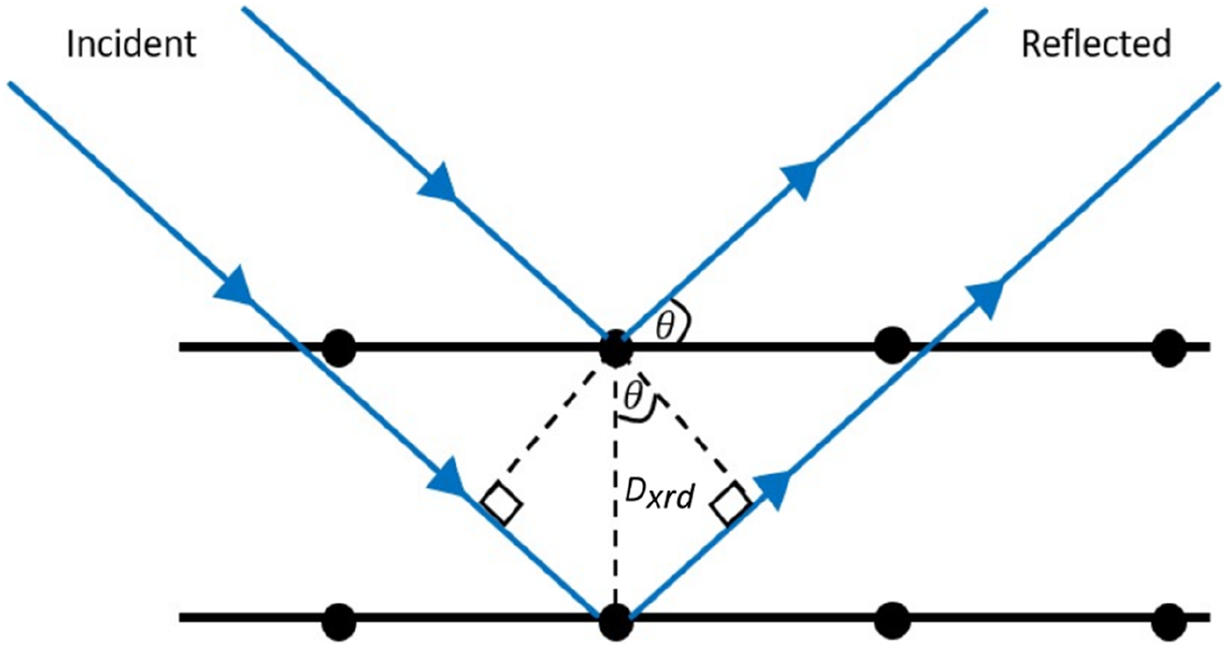
Photoluminescence Piezospectroscopy

Photoluminescence Piezospectroscopy (PLPS) works by subjecting a sample to a laser light of known wavelength. Certain atoms within the sample, depending on the stress state, will be excited and when the atomic system returns to a lower energy state in a time, t of between 10⁻⁹ and 10⁻⁶ s, fluorescence occurs. The wavelength of light emitted is measured as a wavenumber with units cm ⁻¹ and different chemical mixtures have their unique wavenumber “fingerprint” ¹⁰³ which are a series of peaks. This is illustrated in Figure 13. When a material is put into compression, the fingerprint peaks shift to a lower wavenumber. When in tension the peaks’ wavenumber increases. The gradient of the shift is the piezospectroscopic coefficient. Alumina is particularly sensitive to this excitation, so much that Gell et al. ¹⁰⁴ used the PLPS method to detect the presence of α-alumina in thermally grown oxides. This high sensitivity normally limits the stress measurement technique to alumina containing samples. The principle of the PLPS stress measurement is therefore to understand the material fingerprint in an unstressed state, measure the peak shift when stress is present, and from a calibration curve deduce the level of stress within a sample.

Figure 13.

Typical PLPS measurement setup (adapted from ¹⁰⁴ ).

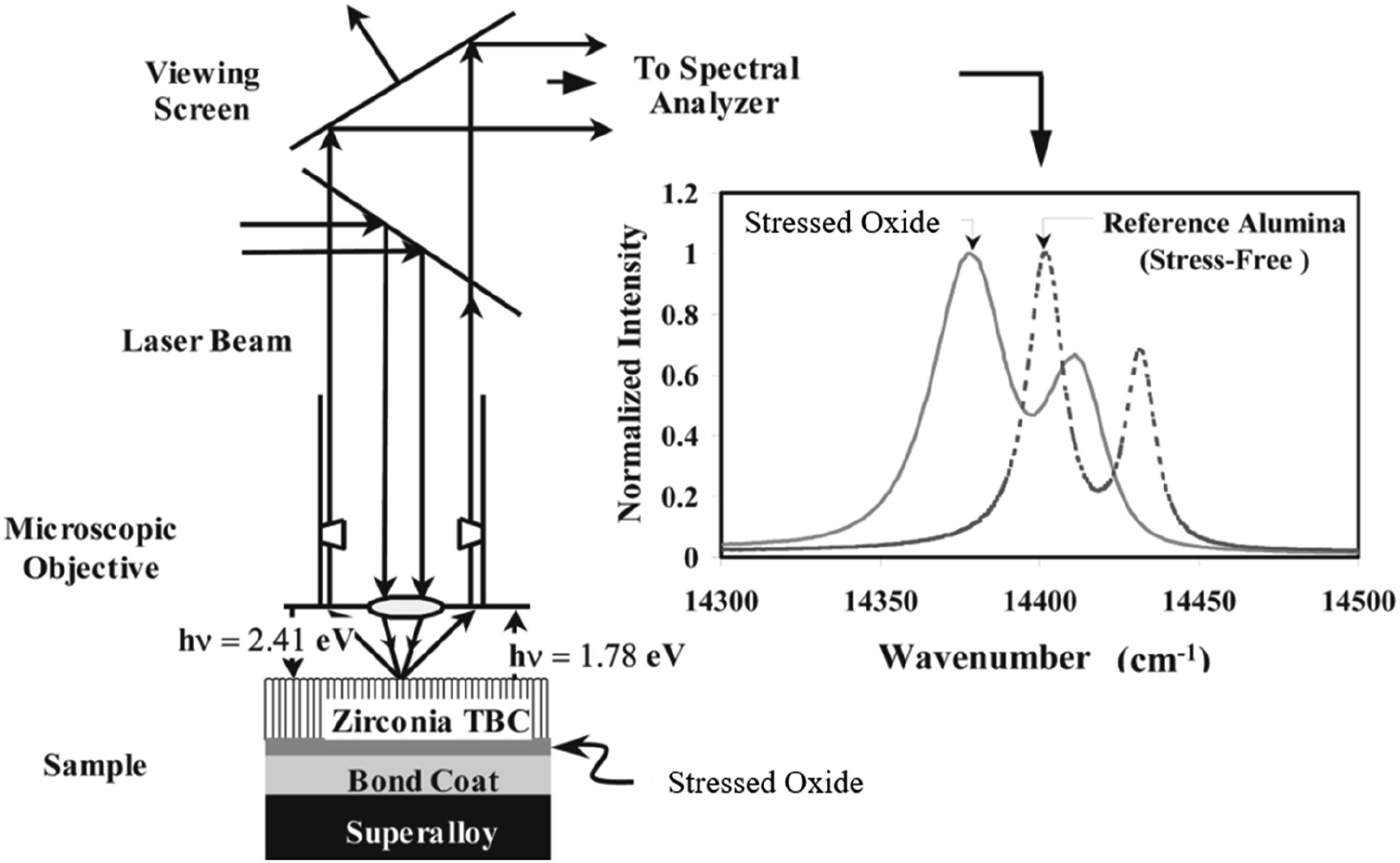
The measurement size depends on scattering of the laser but is estimated to range from 5 to 20 um ¹⁰⁴ up to 500 um. ¹⁰⁵ This is beneficial for measuring small sample patches but also means a scanning procedure would be needed for measurements across a large surface. A typical PLPS measurement system is shown in Figure 13.

Thermite welding is a common welding procedure to join CWR sections, and results in an alumina containing joint. Kim et al. ¹⁰³ used a portable PLPS system signal-to-noise ratio to first confirm that there were high enough concentrations of alumina on the outer face of a weld making the measurement theoretically possible. They then determined the zero-stress fingerprint by measuring a pulverised weld sample, as the powder form cannot contain stress.

Figure 14 shows the results of the PLPS measurement applied to compressed weld samples; there is almost a linear regression within the elastic region. However, up to 50 MPa, the stress range that is often crucial in monitoring NRT, the pattern is not linear and first increases before decreasing. This initial increase is unexpected, as compression is known to decrease wavenumber frequency, and suggests measurement error in the low stress range.

Figure 14.

PLPS wavenumber shift within alumina containing weld samples under increasing compressional load within the elastic region (adapted from ¹⁰³ ).

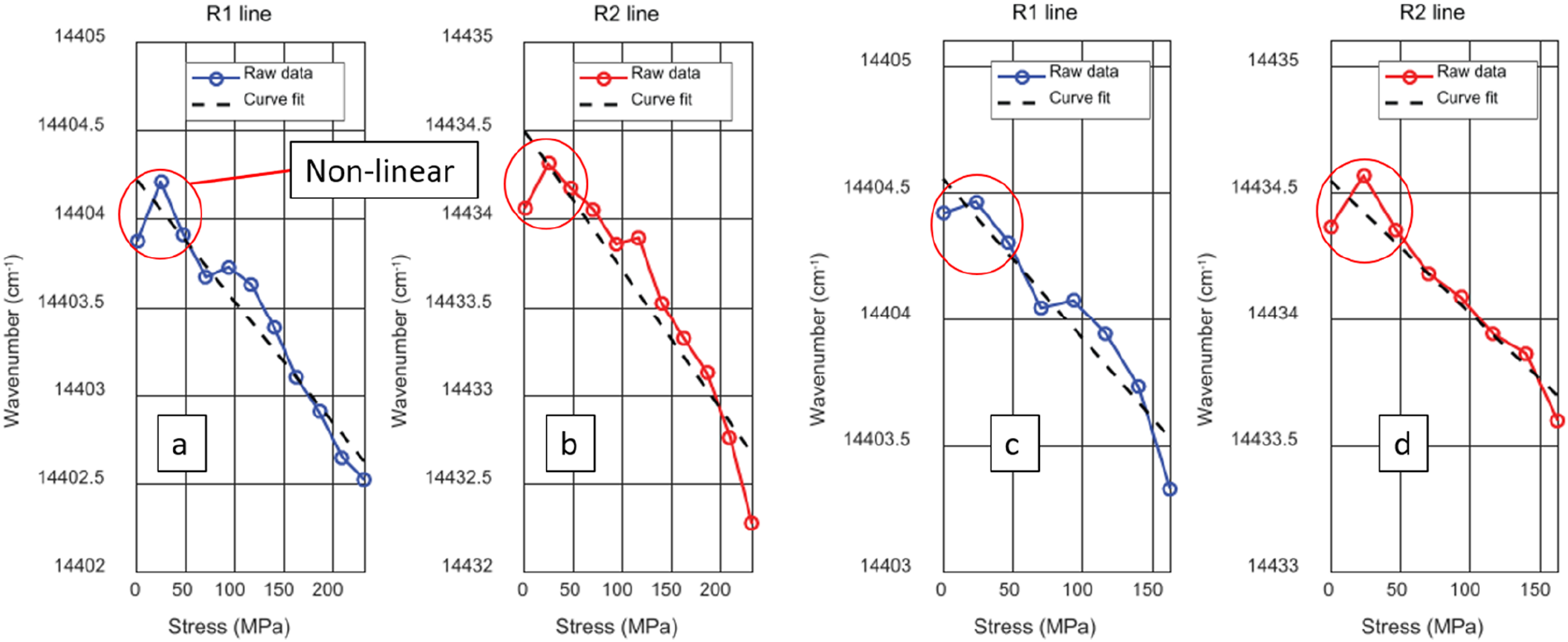
The wavenumber resolution of the portable system used in this study ¹⁰³ was 3 cm ⁻¹ . However, the authors state a wavenumber resolution of −0.0054 cm ⁻¹ is required to see a 1°C change in NRT with a compressional force.

The work was continued by Yun et al. ¹⁰⁵ who applied the portable PLPS system to a large testbed with full scale track sections. Within the study, the piezospectroscopic coefficient was calculated using strain gauge measurements from close to the weld areas, where there is a large amount of scatter about the plotted regression line that the authors attribute to thermal residual stress, welding condition, and micro-structure of the alumina dispersion throughout the weld.

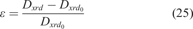
Equation (26) mathematically expresses the PLPS method for stress measurement, where 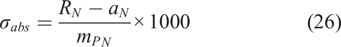${\sigma }_{abs}$ is the absolute stress, $R_N$ is the wave number for peak N, $a_N$ is the zero-stress wavenumber in cm ⁻¹ , and $m_P$ is the piezospectroscopic coefficient in cm ⁻¹ /GPa.

${\sigma }_{abs}=\frac{R_N-a_N}{{m_P}_N}\times 1000$

(26)

The constant $a$ must be determined within a laboratory setting, $m_P$ could also be determined within a lab, or on track if strain gauges are present to compare a stress value to, as was the case in Ref. 105. For NRT measurement, the measured absolute stress is initially plotted against track temperature readings (or alternatively another laboratory-based calibration). A linear weighted least square estimation is then applied to the plot to calculate the temperature at which the rail would be in a stress-free state or the NRT. In the work by Yun et al., ¹⁰⁵ the PLPS method was able to measure the NRT accurate to ±4.9°C.

There are two major advantages for the PLPS method. First, the probe is not in contact with the rail, and measurements can be taken in 0.01 s. ¹⁰⁵ This means future work could mount a PLPS system onto a train to take vast numbers of measurements as the train is moving, rather than operators having to plan maintenance trips to specific track locations. This would provide a huge cost saving and allow for widespread data collection. It also means that surface preparation is not necessary.

The drawbacks to the method, however, are that the PLPS is only sensitive to a weld site, where there is alumina present. This limits measurements to very precise locations and restricts freedom of NRT measurement discretisation along a line. Additionally, the sensing area is very small, within the μm ² magnitude, meaning the measurement is at mercy to determining bulk stress from a very small measurement area. There is also potential for the alumina concentration to be too low at a sensing area, causing the fingerprint magnitude to be reduced and a measurement impossible. Finally, the PLPS measurement system is only applicable to welds where alumina is present, that is just thermite welding. Although this is the most common weld type in the US and is susceptible to PLPS because of the use of aluminium powders, other methods used such as flash butt welding and gas pressure welding are also used ¹⁰⁶ and do not contain alumina particles, making them unmeasurable via the PLPS method.

Discussion

Table 4 summarises all the existing methodologies for measurement of longitudinal thermal stress or NRT. The table outlines the basic operational principles, limitations, reported accuracy in both laboratory and field settings, TRL level and references associated with each measurement method. Measurement accuracies are presented in °C instead of MPa as per industrial convention. Conversion was carried out by assuming a Young’s modulus of 207 GPa and thermal expansion coefficient of 1.15 × 10⁻⁵°C ⁻¹ . The TRL level is evaluated based on NASA’s definition. ¹⁰⁷

Table 4.

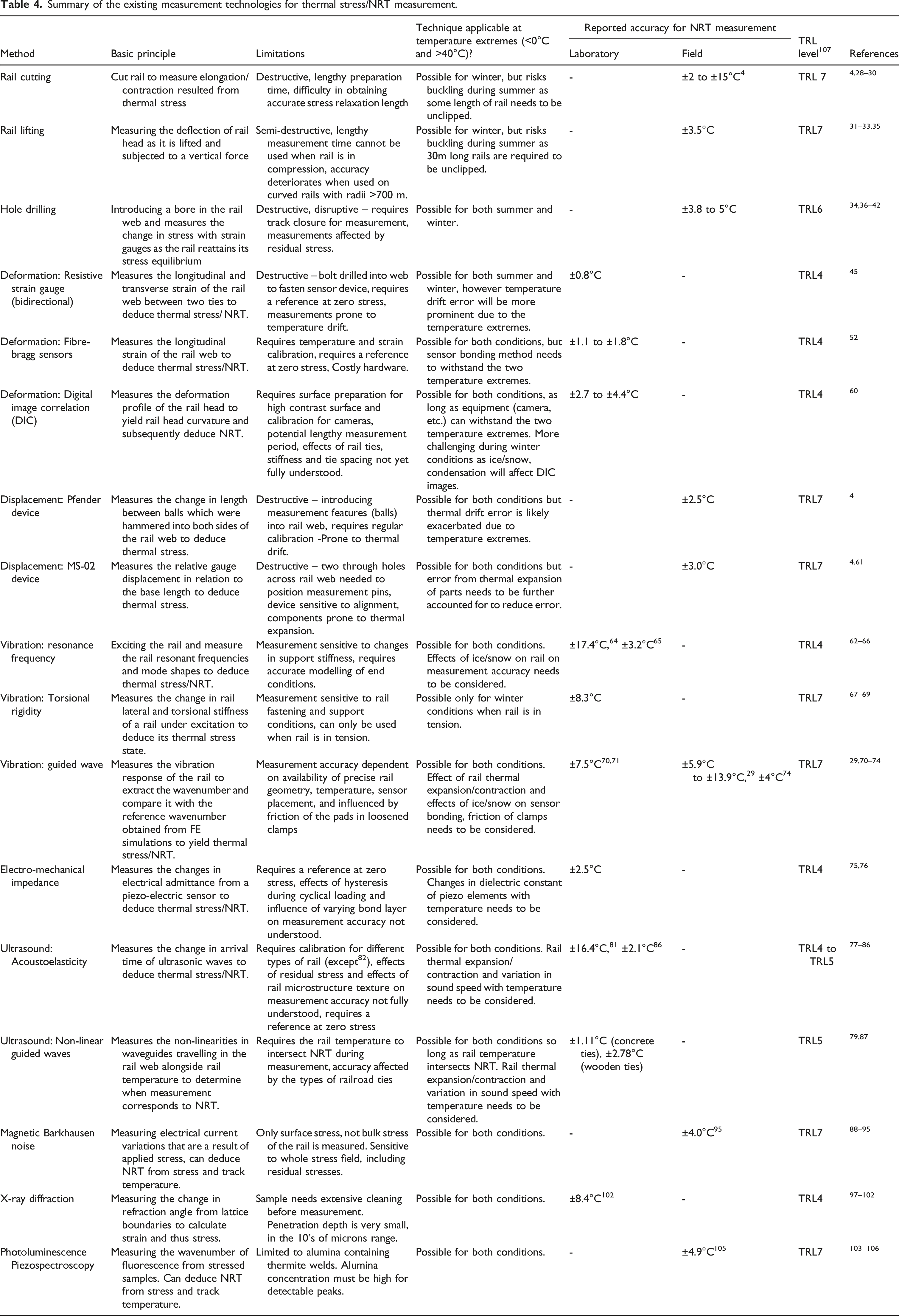
Summary of the existing measurement technologies for thermal stress/NRT measurement.

Method	Basic principle	Limitations	Technique applicable at temperature extremes (<0°C and >40°C)?	Reported accuracy for NRT measurement		TRL level 107	References
				Laboratory	Field
Rail cutting	Cut rail to measure elongation/contraction resulted from thermal stress	Destructive, lengthy preparation time, difficulty in obtaining accurate stress relaxation length	Possible for winter, but risks buckling during summer as some length of rail needs to be unclipped.	-	±2 to ±15°C 4	TRL 7	4,28–30
Rail lifting	Measuring the deflection of rail head as it is lifted and subjected to a vertical force	Semi-destructive, lengthy measurement time cannot be used when rail is in compression, accuracy deteriorates when used on curved rails with radii >700 m.	Possible for winter, but risks buckling during summer as 30m long rails are required to be unclipped.	-	±3.5°C	TRL7	31–33,35
Hole drilling	Introducing a bore in the rail web and measures the change in stress with strain gauges as the rail reattains its stress equilibrium	Destructive, disruptive – requires track closure for measurement, measurements affected by residual stress.	Possible for both summer and winter.	-	±3.8 to 5°C	TRL6	34,36–42
Deformation: Resistive strain gauge (bidirectional)	Measures the longitudinal and transverse strain of the rail web between two ties to deduce thermal stress/ NRT.	Destructive – bolt drilled into web to fasten sensor device, requires a reference at zero stress, measurements prone to temperature drift.	Possible for both summer and winter, however temperature drift error will be more prominent due to the temperature extremes.	±0.8°C	-	TRL4	45
Deformation: Fibre-bragg sensors	Measures the longitudinal strain of the rail web to deduce thermal stress/NRT.	Requires temperature and strain calibration, requires a reference at zero stress, Costly hardware.	Possible for both conditions, but sensor bonding method needs to withstand the two temperature extremes.	±1.1 to ±1.8°C	-	TRL4	52
Deformation: Digital image correlation (DIC)	Measures the deformation profile of the rail head to yield rail head curvature and subsequently deduce NRT.	Requires surface preparation for high contrast surface and calibration for cameras, potential lengthy measurement period, effects of rail ties, stiffness and tie spacing not yet fully understood.	Possible for both conditions, as long as equipment (camera, etc.) can withstand the two temperature extremes. More challenging during winter conditions as ice/snow, condensation will affect DIC images.	±2.7 to ±4.4°C	-	TRL4	60
Displacement: Pfender device	Measures the change in length between balls which were hammered into both sides of the rail web to deduce thermal stress.	Destructive – introducing measurement features (balls) into rail web, requires regular calibration -Prone to thermal drift.	Possible for both conditions but thermal drift error is likely exacerbated due to temperature extremes.	-	±2.5°C	TRL7	4
Displacement: MS-02 device	Measures the relative gauge displacement in relation to the base length to deduce thermal stress.	Destructive – two through holes across rail web needed to position measurement pins, device sensitive to alignment, components prone to thermal expansion.	Possible for both conditions but error from thermal expansion of parts needs to be further accounted for to reduce error.	-	±3.0°C	TRL7	4,61
Vibration: resonance frequency	Exciting the rail and measure the rail resonant frequencies and mode shapes to deduce thermal stress/NRT.	Measurement sensitive to changes in support stiffness, requires accurate modelling of end conditions.	Possible for both conditions. Effects of ice/snow on rail on measurement accuracy needs to be considered.	±17.4°C, 64 ±3.2°C 65	-	TRL4	62–66
Vibration: Torsional rigidity	Measures the change in rail lateral and torsional stiffness of a rail under excitation to deduce its thermal stress state.	Measurement sensitive to rail fastening and support conditions, can only be used when rail is in tension.	Possible only for winter conditions when rail is in tension.	±8.3°C	-	TRL7	67–69
Vibration: guided wave	Measures the vibration response of the rail to extract the wavenumber and compare it with the reference wavenumber obtained from FE simulations to yield thermal stress/NRT.	Measurement accuracy dependent on availability of precise rail geometry, temperature, sensor placement, and influenced by friction of the pads in loosened clamps	Possible for both conditions. Effect of rail thermal expansion/contraction and effects of ice/snow on sensor bonding, friction of clamps needs to be considered.	±7.5°C70,71	±5.9°C to ±13.9°C, 29 ±4°C 74	TRL7	29,70–74
Electro-mechanical impedance	Measures the changes in electrical admittance from a piezo-electric sensor to deduce thermal stress/NRT.	Requires a reference at zero stress, effects of hysteresis during cyclical loading and influence of varying bond layer on measurement accuracy not understood.	Possible for both conditions. Changes in dielectric constant of piezo elements with temperature needs to be considered.	±2.5°C	-	TRL4	75,76
Ultrasound: Acoustoelasticity	Measures the change in arrival time of ultrasonic waves to deduce thermal stress/NRT.	Requires calibration for different types of rail (except 82 ), effects of residual stress and effects of rail microstructure texture on measurement accuracy not fully understood, requires a reference at zero stress	Possible for both conditions. Rail thermal expansion/contraction and variation in sound speed with temperature needs to be considered.	±16.4°C, 81 ±2.1°C 86	-	TRL4 to TRL5	77–86
Ultrasound: Non-linear guided waves	Measures the non-linearities in waveguides travelling in the rail web alongside rail temperature to determine when measurement corresponds to NRT.	Requires the rail temperature to intersect NRT during measurement, accuracy affected by the types of railroad ties	Possible for both conditions so long as rail temperature intersects NRT. Rail thermal expansion/contraction and variation in sound speed with temperature needs to be considered.	±1.11°C (concrete ties), ±2.78°C (wooden ties)	-	TRL5	79,87
Magnetic Barkhausen noise	Measuring electrical current variations that are a result of applied stress, can deduce NRT from stress and track temperature.	Only surface stress, not bulk stress of the rail is measured. Sensitive to whole stress field, including residual stresses.	Possible for both conditions.	-	±4.0°C 95	TRL7	88–95
X-ray diffraction	Measuring the change in refraction angle from lattice boundaries to calculate strain and thus stress.	Sample needs extensive cleaning before measurement. Penetration depth is very small, in the 10’s of microns range.	Possible for both conditions.	±8.4°C 102	-	TRL4	97–102
Photoluminescence Piezospectroscopy	Measuring the wavenumber of fluorescence from stressed samples. Can deduce NRT from stress and track temperature.	Limited to alumina containing thermite welds. Alumina concentration must be high for detectable peaks.	Possible for both conditions.	-	±4.9°C 105	TRL7	103–106

Most of the methods discussed share two common limitations. These are the major bottlenecks for quick and reliable NRT measurements. The first is the need for a stress-free calibration signal, so that any measurement can be zero-offset to deduce the thermal stress. Theoretically, this can be alleviated by testing on an unstressed rail sample in a laboratory setting to generate a set of stress-free calibration data or curve. However, the laboratory rail sample might differ from those in the field as residual stresses could be induced during sample preparation. Additionally, railway tracks potentially differ in their material properties depending on their grades, manufacturing location/batch and age as well as the changes the rails experience during operation. All these add a complex dimension to field NRT measurement. A potential solution is to generate a database for the most common rail grades in service and zero-stress calibrate through statistical means. The database will however be specific to a certain setup for a certain technique and will involve a sizeable testing campaign.

The second major challenge is attributed to the relatively low thermal stress (<60 MPa) induced in the rail. Such a low stress measurement requirement automatically disqualifies methods with inadequate sensitivity and places utmost importance on reducing signal noise to ensure measurement accuracy and consistency. Reduction in instrument noise could be achieved through hardware improvements such as more robust casing, cable shielding and higher frequency data sampling devices. This typically translates to requiring expensive, high-performance sensing hardware. Software advances such as embedding Artificial Intelligent (AI) and improvements in post-processing algorithms could also facilitate improvements in measurement accuracy and time.

VERSE remains the industry standard despite its limitations and semi-destructive nature, and it is the sole method with appropriate TRL level suitable to be deployed on rails. However, some notable non-destructive technologies for NRT measurement include the electro-mechanical impedance method, the ultrasonic non-linear guided waves method and the ultrasonic acousto-elasticity method. All these methods have been trialled in laboratory conditions with the ultrasonic non-linear guided waves method and the electro-mechanical impedance method having comparable accuracy at around ±2.5°C. Despite this, the ultrasonic non-linear guided wave method requires a lengthy measurement window, and its accuracy fluctuates depending on railroad ties. Conversely, the electro-mechanical impedance method requires a zero-stress measurement and further understanding on the effects of bond layer and hysteresis on measurement accuracy. The ultrasonic acousto-elasticity method lacks comprehensive study to quantify its accuracy and limitations.

Clearly, the aforementioned issues need to be resolved for any of these methods to be adopted for field NRT measurements. Furthermore, practical considerations are also necessary. This includes minimising pre-measurement preparation to reduce maintenance time, disruption and cost and potentially retrofitting sensors (once proven to appropriate TRL levels) onto moving carriages to facilitate measurement across rail networks. A moving measurement system would develop a larger database, enabling improved modelling of track conditions, and further development of data-driven predictive maintenance models.

In the authors opinion, future developments on NRT measurement should focus on four key criteria: improving measurement consistency and accuracy, methods of reliable calibration, and reducing measurement speed to minimise service disruptions. These are applicable across all the sensing methods discussed within this paper. Advancing NRT methods is essential for ensuring efficient railway operations, a key component of the UK’s strategy to attain net-zero emissions by 2050, ¹⁰⁸ with rail transport recognized as the cleanest commuting method.

Conclusions

While a variety of techniques have been developed across a wide range of principles, none of them have yet fully met the ideal criteria for thermal stress/NRT measurement. VERSE remains the industry standard due to its reliability, precision, and convenience. However, it is semi-destructive in nature, time consuming, cannot be used on curved track and must be applied when in tension, meaning night-time measurements are most common. Therefore, there is still high demand for alternative technologies to take NRT measurements.

Alternative methods, despite not meeting all the specified criteria, still offer a satisfactory accuracy. For instance, utilising the Rail-NT system (non-linear guided waves) allows for NRT measurement at acceptable accuracy in the field however at the expense of potential lengthy measurement times. It is evident from this study that, at the current state, no single technique is able to satisfy the “ideal measurement criteria”, however these methods can still be implemented provided that their operational limitations are fully understood.