A laser scanner based approach for identifying rail surface squat defects

Abstract

The defect identification process within the UK rail industry has seen significant improvements over the past decade with the introduction of new measurement systems and defect detection systems. Although significant work has been on the defect identification little work has been done on the process after the defect has been detected. This repair process is still extremely manual. Due to the current process being manual the repair operation has very little traceability and transparency. This paper has therefore presented the need for not only a defect detection system but a defect repair system for the UK railway industry. Further to this, this paper has acknowledged that the rise of defects occurring on the UK railway lines requires a solution that can fully repair a defect with little to no user intervention in a timely manner. To address this, this paper has taken the extremely manual process of rail repair and has laid out the possibilities to automate this process. By doing this a work flow diagram has been generated to show how the system could be used to repair surface defects with a specific focus being made on squat defects. To achieve this a defect detection and measurement system has been explored, as this will make up the first stage of the automated repair system. The literature on various defect detection algorithms was reviewed and two variations of existing defect detection algorithms were created, i.e. the Covariance method and the Normal Intersection method. These algorithms have been tested against 100 simulated squat defects and have been verified using 4 experimentally generated defects. Both algorithms have been proven to not only identify the approximate size of the defect but also its location. This successful defect identification will be integrated into an automated rail repair system.

Introduction

The ability to subtract and add material using one integrated system is of particular interest during remanufacturing or repairing operations. This is because these processes allow parts to increase their life with a significantly reduced cost when compared to replacing the component particularly with more expensive components such as railway track. These operations are also referred to as reincarnation operation due to the effect of giving the component ‘new life’.^1,2 This type of system could be used for repairing in service defects caused by wear propagation or damage. This paper will examine the use of such a system within railway applications particularly focussing on track surface defects. Over the last few years’ significant effort has been made to automate the defect detection process to streamline and reduce cost of track maintenance, through the introduction of Network Rails test trains, including the NMT commissioned in 2003 and the Ultrasonic Testing Unit train (UTU). Substantial changes have been made to on the board equipment and the systems used over the recent years, including the introduction of the Plain Line Pattern Recognition (PLPR) system, which is used to help detect missing components and take images of the joints and track for offline inspection. Although significant advances have been made in utilising various technologies, there is still work to be done on automating both the detection process as well as the repair process. This increased interest in analysing existing rail

tracks and repairing the damage instead of replacing the rail is largely due to the limited available down time within the rail network due to delay charges and track availability requirements. This has been the key drivers for the creation and development of a rapid and high integrity repair system. This has become increasingly important due to the exponential relationship between track maintenance cost and track age. ³ Such systems can be seen within the light rail industry, where the track is encased in a polymer. Here a semi-autonomous process is used in the repair of work rails. The repair process uses submerged arc welding, to build-up worn grooved rail to restore it to an operational condition.

Surface rail defects are a large contributor to the cost of track maintenance. In the Netherlands, around €5 000/km is spent each year on squat defects alone. ⁴ A report published by In2Rail showed that network rail found approximately 6300 defects within their network between 2015 and 2016 with over 5000 defects being diagnosed as squat defects. ⁵ Although the cost of the repair of these defects isn’t clear from this report a paper published by the Transport Research Arena estimated the cost to be between €30 000 and €10 0000 per km per year for a modern European railway track. ⁶ A further Network Rail report also stipulates that the number of defects being identified outweighs the number of defects being fixed and this trend is true for the previous 4 years, meaning that, as the infrastructure ages, defect repair will become even more critical than it currently is. ⁷

Due to the high occurrence of squat defects, as discussed above, the focus of this paper is on the detection with the ultimate goal of creating a repair process of squat defects. Squat defects are initiated by either a small subsurface crack or small surface indentation on the rail. ⁴ Although many authors have speculated to the cause of squat defects there is little consensus within the research community on the root cause of these defects. However it is widely acknowledged that squat defects begins with a sub-surface or near surface crack that propagates in manner which lowers the structural integrity of the rail causing a visual depression in the rail hence the name squat. A squat defect is usually quite easy to spot as it is a depression on the track, similar to if a ‘heavy gnome’ sat on the track hence the name “squat”. ⁴ However, due to their appearance they can often be confused with wheel burn which, rather than occurring slowly over time, occurs instantly with wheel slip. ⁸ The location of squat defect is very specific only occurring on the running surface of the rail as shown in Figures 1 and 2.

Figure 1.

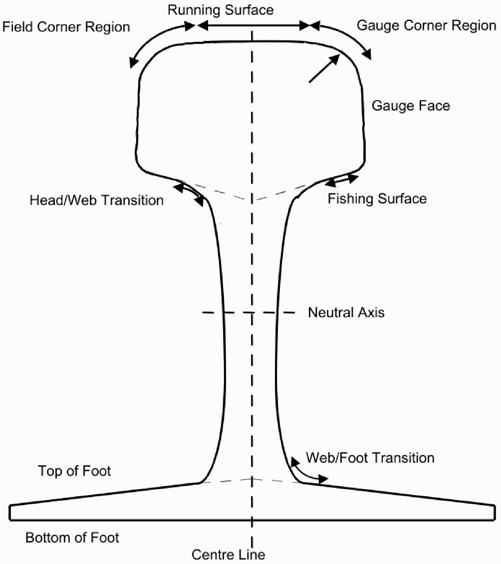
Schematic of a rail profile including main areas. ⁸

Figure 2.

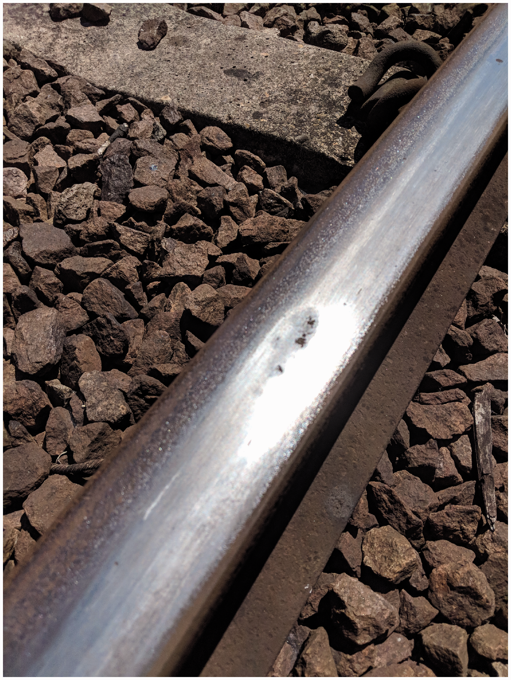
An example of a squat defect near the GCR Quorn railway station.

A squat defect is typically labelled as such, once it has exceeded a critical size, which, within the EU, is between 6 mm and 8 mm. ⁴ An example of such a defect, taken at the GCR Quorn Railway station, Leicestershire can be seen in Figure 2.

Currently track repair in the UK starts with the use of Network Rail’s test trains including the NMT commissioned in 2003 and the Ultrasonic test Unit. This is coupled with the use of hand held Sperry ultrasonic test equipment which is used to identify and measure internal defects on much more local level. These test trains are used to test the physical infrastructure of the railway lines including overhead lines and tracks. The NMT train uses the PLPR system and various sensors including transducers and accelerometers to measure the track geometry, track alignment and to identify missing components, but currently is not capable of automatically measuring or detecting surface or sub surface defects. While the UTU uses ultrasonic transducers to estimate the size and shape of internal defects. This has led to various authors to investigate the use of these sensors or similar sensors to measure defect size and locations.^4,9,10 Furthermore, the NMT utilises laser scanning and single camera pattern recognition edge detection to identify and flag possible defects which are then inspected by experts. Examples of these various defect detection approaches can be seen in the work completed by Molodova et al., Rikhotso et al., and Ye et al. which all showed the use of a laser line scanner in order to identify surface defects.^4,10,11

Existing approaches published within literature have tried to address the same problem of how the NMT can identify surface defects by attaching a laser line scanner to the existing NMT equipment. However, the repair process after the defect has been found is still a very manual process. As shown by the In2Rail project the currents state of the art is the welding and machining system named Discrete Defect Repair developed by ARR, although there are many positive of this system including the lower preheat temperature and the traceability of the process, it has not solved the need to locate the defect locally. The current process employed by Network Rail includes having a team of operators undertake the local defect verification, the removal of the defect or section of track and then the final welding of the track. ¹² This manual process is slow, dangerous to the operators performing the defect repair and gives little traceability to the repair process and therefore forms the focus of this paper. ‘Repair system architecture’ section of this paper outlines, for the first time a system which can utilise the information gathered by a primary defect identification system such the ones developed for the NMT and the PLPR systems to pass the approximate defect location to a rail based autonomous repair ’bogie’, as described in Figure 3. Eventually the proposed system would not only identify a defect flagged for repair, as suggested in this paper, but also be able to remove the defect and additively add material back to the track returning it to its running condition. The benefit of this would be two, fold; firstly it decreases risk to human life by minimising the amount of people on the track, secondly the repair and all the parameters surrounding the repair could be logged and tracked thus increasing the traceability of the repair. This could further feed into a mapping system which keeps track of the current state of the rail infrastructure.

Figure 3.

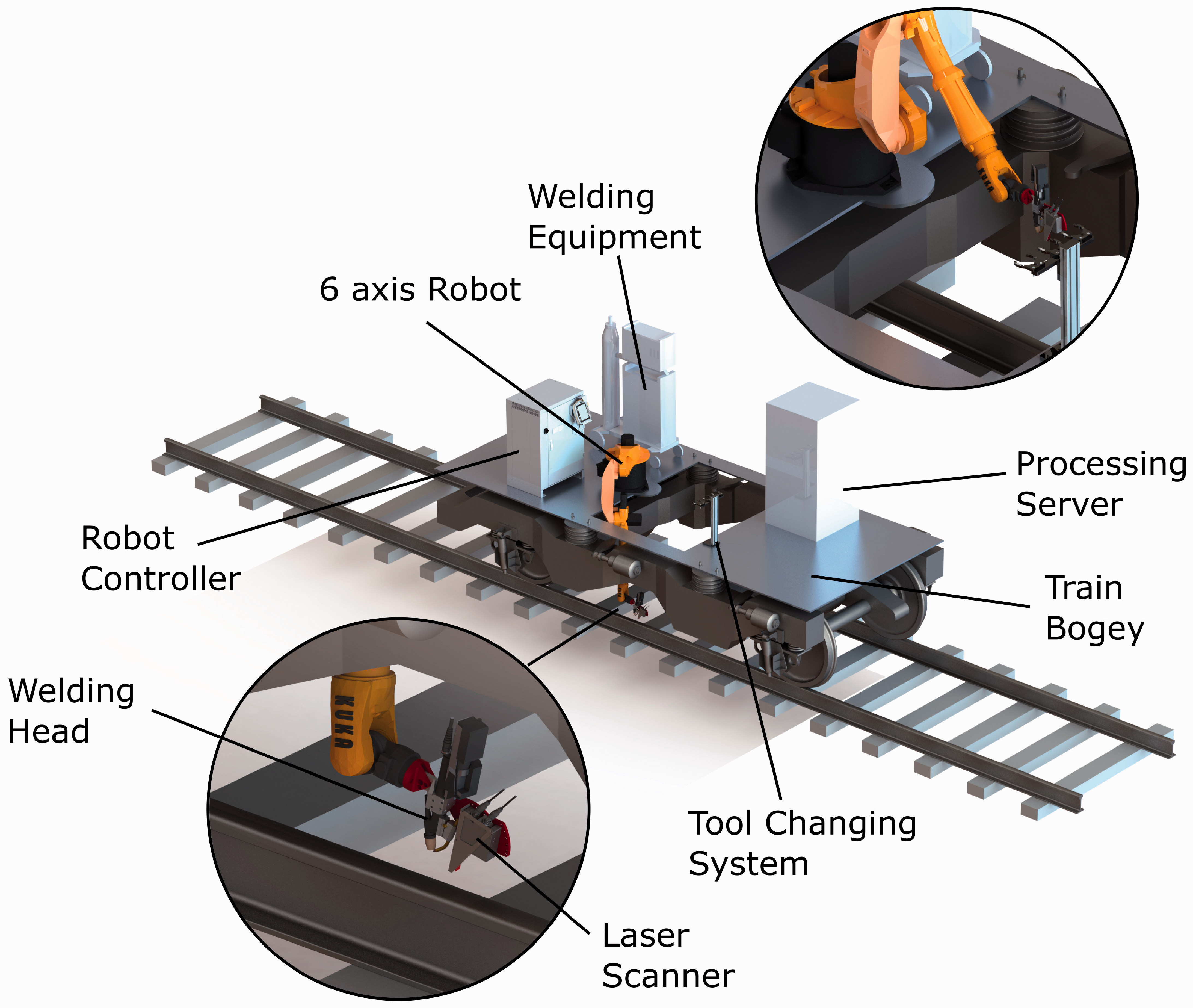
Schematic of the propose solution for the rail repair system.

Repair system architecture

The repair system has been split into its three main constituent parts, a defect identification system, a material removal system and an additive manufacturing system. This paper focuses on the preliminary design of the autonomous track repair system and the inspection subsystem within it. The repair system described in this paper would require Network Rail to be capable of identifying the approximate location of surface defects, this could be done using a number of available test trains, including the NMT and the UTU, or the use of the Sperry ultrasonic sensors. Once the primary identification of the defect has been completed then the repair system can be planned into the railway operations, similar to how the current manual process is completed. The purpose of this system would be to locate the defect flagged by Network Rail for repair and remove the defective material, build material back to the required height and then grind back to finish. Within this paper a focus has been made on developing a robust squat defect detection algorithm building on the work done by Ye et al., ¹⁰ testing these algorithms on a large number of simulated defects and verifying the two algorithms on experimental defects. The 100 simulated defects were positioned onto a modelled piece of 60E2 rail, randomly changing the size and location of each defect, this is discussed in detail within ‘Simulation of scanner data’ section. Furthermore, Figure 3 shows a schematic of the proposed final system solution consisting of a 6 DOF industrial robot placed on a bogie which can be locked in place, with Figure 4 showing the process flow of the whole repair operations. A tool changer is used to allow the system to change between a laser line scanner, industrial grinder and a MIG welding system, which would be used for the defect identification, defect removal, material deposition and the finishing operation. This would enable autonomous changing from detection to strategic repair.

Figure 4.

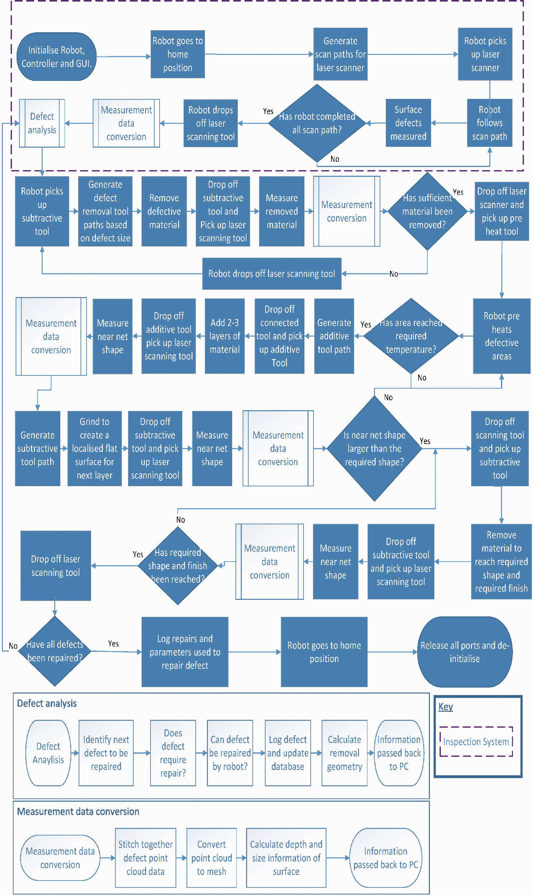
Flow chart showing the work flow of an autonomous rail repair system.

A laser line scanner was shown by Ye et al. to be very good at measuring and identifying squat defects. A laser scanner allows for a 3 D profile of the defect to be created and therefore estimate the amount of material which is required to be removed, however once the material has been removed a rescan would have to occur to both verify the geometry of the weld prep created and also check for any sub surface defects which may have been uncovered during the removal process. The amount of material will be primary driven by the size of the defect however careful consideration will also be made to the British Standard BS 15594:2009 ¹³ which defines minimal material removal requirements. Once the material has been removed further scanning is required to check the welding surface which may have revealed subsurface cracking not previously visible. A grinding unit was chosen as this would allow for the simple removal of the defective area while minimizing the stiffness requirements of the robot. Furthermore, the current manual repair process utilises a grinder for the blending of the rail. ¹² To reduce the impact of the additional interfaces with the parent material which would increase the complexity of the welding joint, the defect removal process of the repair process will remove not only the defect but remove the whole width of the rail head. Finally a report delivered by the Manufacturing Technology Centre (MTC) to the London underground showed that a Cold Metal Transfer (CMT) MIG welding unit was the most suitable welding process for the rail repair application. ¹⁴ Although there are some advantages of having a manual system compared to a fully automated system such as the flexibility of a human to adapt and adjust a fully automated system allows for a much safer environment and a much more transparent repair process with increased traceability.

A detailed flow diagram is presented in Figure 4 which shows the full system architecture details and shows how the final system should be used. The essence of the flow chart describes how the system will identify and detect a defect within a region defined by Network rails NMT. The flowchart goes on to describe how the defect would be removed and how the new material would be added. The flow chart further describes how the systems switches between the inspection tool, material removal and deposition tool in order to validate the each process is happening as expected and that any slag or impurities created during the deposition process can be removed. Although the final solution is an automated rail repair system each subsystem must first be developed and tested therefore the focus of this paper is the section highlighted with a dashed box in Figure 4, with particular focus on locating and detecting the defect. The flow chart shows how the system will operate and could be used for both understanding the process flow as well as being used for a high level software architecture.

Methodology

In order to show that it is possible for a robotic arm to be used as an autonomous repair system; first each individual subsystem must be proved. As mentioned in ‘Simulation of scanner data’ section the purpose of this paper is to prove the viability of using an industrial robotic arm to locate surface defects within a predefined area. To achieve this a defect detection algorithm was developed and thoroughly tested on 100 simulated defects and validated on 4 real test samples as shown in Figure 9. The process of creating this simulation included the creation of an ideal model of piece of 60E2 rail, a squat defect was then procedurally generated and implanted into the rail. On generating this now defective piece of rail the laser scanner point cloud data was simulated and the point cloud was handed to the defect detection algorithms, this is discussed in detail within ‘Simulation of scanner data’ section. Due to the number of defects required to fully test whether an algorithm is robust, a simulated approach was used with a real world verification step. This methodology utilised 100 simulated squat defects in order to statistically determine the accuracy of the defect detection algorithms. Once the algorithms had been tested on a large number of simulated defects, then the algorithm was validated on real test samples. Two different detection algorithms were developed both of which are variants of the algorithms discussed in the paper produced by Ye et al. ¹⁰ Although similar to the ones described by Ye et al. significant changes have been made including some improvements making the algorithms more generic for a wider range of squat and surface defects. Within this paper the coordinate system of the rail has been kept in keeping with BS EN 13848-1:2019 ¹⁵ and can be seen in Figure 5.

Figure 5.

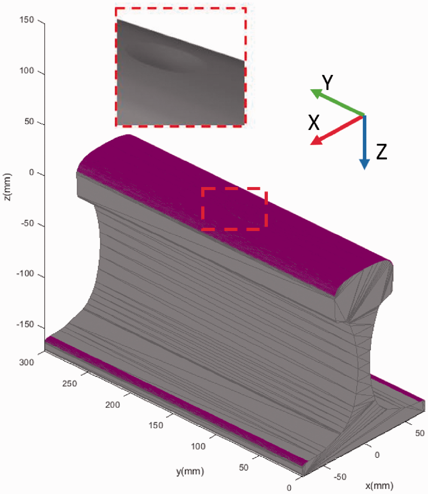
Model of a 60E2 rail with a length of 300 mm taken from the BS13674-1 ²¹ including generated point cloud data.

Equipment used

In order to complete the real world testing, a Micro Epsilon 2900-100BL laser line scanner ¹⁶ was used in conjunction with a KUKA KR16 utilising a KRC2 controller. The Micro epsilon laser line scanner uses the triangulation technique to measure the distance both along the laser stripe and the distance collinear to the laser line. The controller used two KUKA robot packages including KR-XML which was used to drive the robot to the required positions and Robot Sensor Interface (RSI) which was used for real time robot communication. The robot and laser line scanner where controlled from an external PC using a bespoke LabVIEW program with a state machine architecture. The state machine allows for new actions to be added easily while maintaining simplicity in the debugging and planning process as each action of the repair process can be defined by an individual state within the state machine. The state machine used to control the repair system allowed for the various robot parameters to be set, including the current tool and base coordinate system, as well as having the ability to use the Micro Epsilon SDK which allowed full control of the capture frequency, laser line length and capture mode of the laser line scanner.

Use of a laser line scanner with a robotic arm

In order to gain a 3 D profile of the track, first the 2 D laser line points must be transformed into the robot’s co- ordinate system. Knowing where the laser scanner is in relation to a base coordinate system is known as the hand eye calibration problem. ¹⁷ The method used within this work to gain the hand eye transformation was the fitted plane approach.^18,19 This is where a plane is scanned at various joint angles, covering as much of the working volume as possible. These scans are then handed to a non-linear solver which attempts to reduce the error of a fitted plane to the scans by adjusting the 6 hand eye calibration values. These include three rotations (α, β, γ) and three translations (x, y, z). The rotation and translations are then put back into the robot controller as the transformation matrix for the tool, alternatively, it can be used offline as a further transformation after the scans have been completed. In order to gain a good hand eye calibration using this method it is important to have first have an estimate of the transformation thus allowing the optimisation model to find the global minima rather than getting stuck in a local minima. This estimate was achieved by teaching the rotations of the tool using KUKA’s 4-point method. ²⁰ This method requires the robot to be driven to the same point in space from 4 different directions and thus allows the rotations to be calculated. To estimate the translations the CAD geometry of the laser scanner bracket was used as this allowed for a good estimate to then use the optimisation technique described here.

There are numerous ways that a laser line scanner and Laser scanner position can be aligned within a gantry or robotic manipulator system. In particular the three methods that have been previously explored include the point to point method, the interpolation methods and the time stamp method. ¹⁸ These methods can reduce the reliance on real time data communication while maintaining accurate scanning data without the need for interpolating individual points. The positives and drawbacks of each of these methods were previously explored in detail in De Becker et al. ¹⁸ With this in mind it was decided that, due to the simple scan path required and the time delay requirement of the time stamp method, the interpolation method would be the best approach. This allowed for a fast capture rate making sure that the simulated point spacing was comparable to the real world point cloud density.

Simulation of scanner data

In order to simulate the scan data first the rail profile was generated and the scan data simulated. This was done by taking a rail profile from BS13674-1 2014, which is typically used within the UK rail network. ²¹ From this standard the rail profile 60E2 was chosen as this was the same profile which was available within the laboratory setting and would therefore provide the best representative simulation for the real world testing. The track which was generated was 300 mm long. It should be noted that if it was proven that the accuracy of the NMT was such that this search area had to be increased or decreased then this could be done very simply. An image of the rail used within the simulation can be seen in Figure 5.

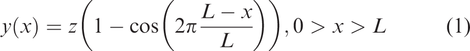
A squat defect was then implanted into the rail using Blender, a free open source piece of software which can be used for STL manipulation. ²² The defect itself was modelled using the British Standard (BS EN 13848-6:2014) for vehicle response analysis. ²³ Although this equation was designed to be used for multi body simulations, it was used in this case as a good representation for the shape of a squat defect in the longitudinal or Y direction. Due to this model being designed for vehicle response measurements model being designed for vehicle response measurements there is no equation for the x or transverse direction. With that in mind it was assumed that the same equation used for the Y direction could be used for the X direction. The equation taken from the British Standard can be seen in equation (1).²³

$$y\left(x\right)=z\left(1-\cos \left(2\pi \frac{L-x}{L}\right)\right),0>x>L$$

(1)

This defect was then scaled and positioned randomly on the 300 mm piece of rail using Blender The random location and scale allowed for the algorithm to be realistically tested without having to measure 100 real world defects. An example of one of the sections of track with an inserted defect can be seen in Figure 5.

The range of defects generated were between 7 and 24 mm in the X direction, 2 mm and 50 mm in the Y direction and finally 0.4 mm to 1.9 mm in the Z direction. This range of defect sizes were taken from literature as representative sizes. Kerr et al. show that a mild to moderate squat defect is between 14.4 mm and 37.4 mm in the transverse (X) direction and between 17.3 mm and 49.0 mm along the longitudinal direction (Y). ²⁴ While Li et al. showed that defects smaller than 5 mm to 6 mm in length would be eroded by wear while a defect of 10 mm in length would grow into a larger squat; in this case growing from 35 mm to 42 mm in width. ²⁵ Finally two papers which attempted to detect squat defects using axle box acceleration (ABA) by Molodova et al. and Yin et al. used test cases of squat defects ranging from 15 mm to 61 mm in length and 0.5 mm to 2 mm in depth.^4,9 Therefore, using all these sources a wide range of defect sizes were chosen in order to capture the full range of possible squat defects. The co-ordinate system used to define the axis can be seen in BS EN 13848-1:2019 and in Figure 5. ¹⁵ These numbers are then verified by Network rail in the In2Rail report, which stated that between 2011 and 2016 the majority of squat defect were less than 51 mm in the Y direction and over a third of defects where less than 10 mm deep. ⁵

Once the squat defects were generated and inserted into the rail within the simulated, a realistic point cloud of the part was generated. This was done by modelling the laser scanner being used during the laboratory testing of the real rail part. The modelling included the measurement range and field of view of the laser scanner. An image of the simulated point cloud generated by the laser scanner can be seen in Figure 5, where the Co-ordinate system shows the origin of the laser line scanner during a single simulated line scan. The point cloud was generated at 0.5 mm increments with a field of view of 45°, and 1280 points per line.

Squat defect detection

Ye et al. discussed three methods to detect squat and gauge corner defects. These methods worked well, however it required a region of interest to be specified before the algorithms could be used. Due to not knowing exactly where the defects are, it was not possible to use this method for unknown defect locations therefore a different version of the FND (Face Normal based) method and depth gradient based method were developed. ¹⁰ These were named as the covariance based approach and the normal intersection approach.

Covariance approach

Firstly a variation of the depth gradient based method was developed utilising the Eigenvector vector of the covariance matrix. The Eigenvector of a covariance matrix identifies the general trend of the data over a specific neighbourhood. This is similar to a depth based gradient approach described by Ye et al., ¹⁰ however, it is much less susceptible to noise as it looks at a larger neighbourhood of points instead of a gradient. This method is also responsive to changes in all directions not just a change the Z direction. This allows this method to be used even if there are missing data points, such as during self-blinding operations. It can also be used if the laser scanner isn’t aligned parallel to the running surface. Furthermore, as this method does not compare the gradient to a known plane, it can measure changes on the gauge corner where the natural gradient of the rail occurs. The neighbourhood radius chosen was 3 mm as, during preliminary testing, this was shown to have the greatest trade-off between computation time and accuracy.

Normal intersection approach

The second method that was explored was the normal intersection approach. However, unlike the FND approach described by Ye et al., this method did not require Delaunay triangulation. This was due to the normals being generated using the 10 nearest neighbours instead of generating faces. ¹⁰ However, in order to speed up the computation time some sub sampling was required. The point clouds were sub- sampled at 3 mm to estimate the approximate location of the defect, the area of interest was then grown by 2 mm in both the x and y direction and the algorithm was rerun on this area with a sub-sampling rate of 1 mm. This was then repeated a third time growing the new area of interest by 0.5 mm and sub sampling at 0.5 mm in order to find the exact area of the defect.

The face normal method described by Ye et al. showed that when the normal of the face exceeded 12° from a reference plane, this was then deemed to be the edge of a defect. This leaves a large amount of uncertainty particularly if the reference plane isn’t parallel to the running surface of the rail head. To overcome this, a variation on this method was developed. This variation utilises the fact that as the defect occurs in the rail, the Euclidean distance between the vectors should decrease and the number of intersection between these normal vectors should increase, with the maximum number of intersection occurring at the centre of the defect. Figure 6 shows a cross section of the rail mesh with a sub- sampling of the normal vectors. Figure 6 also shows that the normal vectors associated with the defect point towards each other while the vectors on the rail point away from each other. This method required that the Euclidean distance was measured so that the intersection could not occur below the surface of the rail and that the vectors were pointing in the positive Z direction. The latter was achieved by completing a dot product of a vector in the desired Z direction with each of the normal vectors. The normal vector was then inverted if the dot product results was negative.

Figure 6.

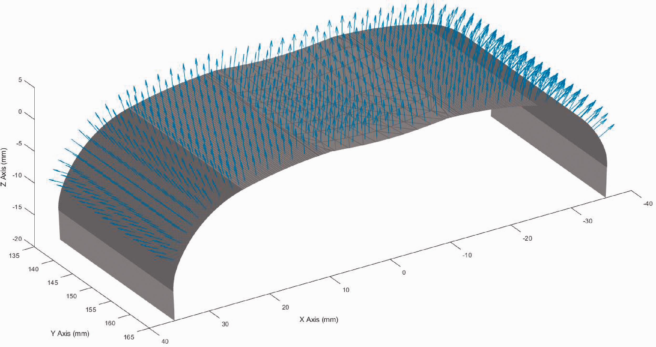
Image of intersection of surface normals.

Simulation results

The graphs shown in Figure 7(a) to (c) show the location and size error for 100 of the simulations which were completed. All the defects which were simulated were detected for both the Face Normal Intersection method and the Covariance method. Figure 7(a) to (c) and Table 1(a) show the location error of the defect found against the defect or simulation number. The simulated defects were all placed at random Y positions, a position of X equal to zero and a z value so that the top of the defect conformed to the existing rail profile as described in ‘Simulation of scanner data’ section and by Figure 5. The graphs in Figure 7(a) to (c) and Table 1(a) show that the location accuracy of the covariance method is significantly higher than the normal intersection method with the covariance method being more consistent as shown by the lower standard deviation, with only a few outlier as shown in the x and z measurements in Figure 7. This higher accuracy is most likely due to errors associated with the generation of the point normals and the sub sampling of the data points within the normal intersection method. Although the range of the error is quite high it should be noted that the standard deviation for both

Figure 7.

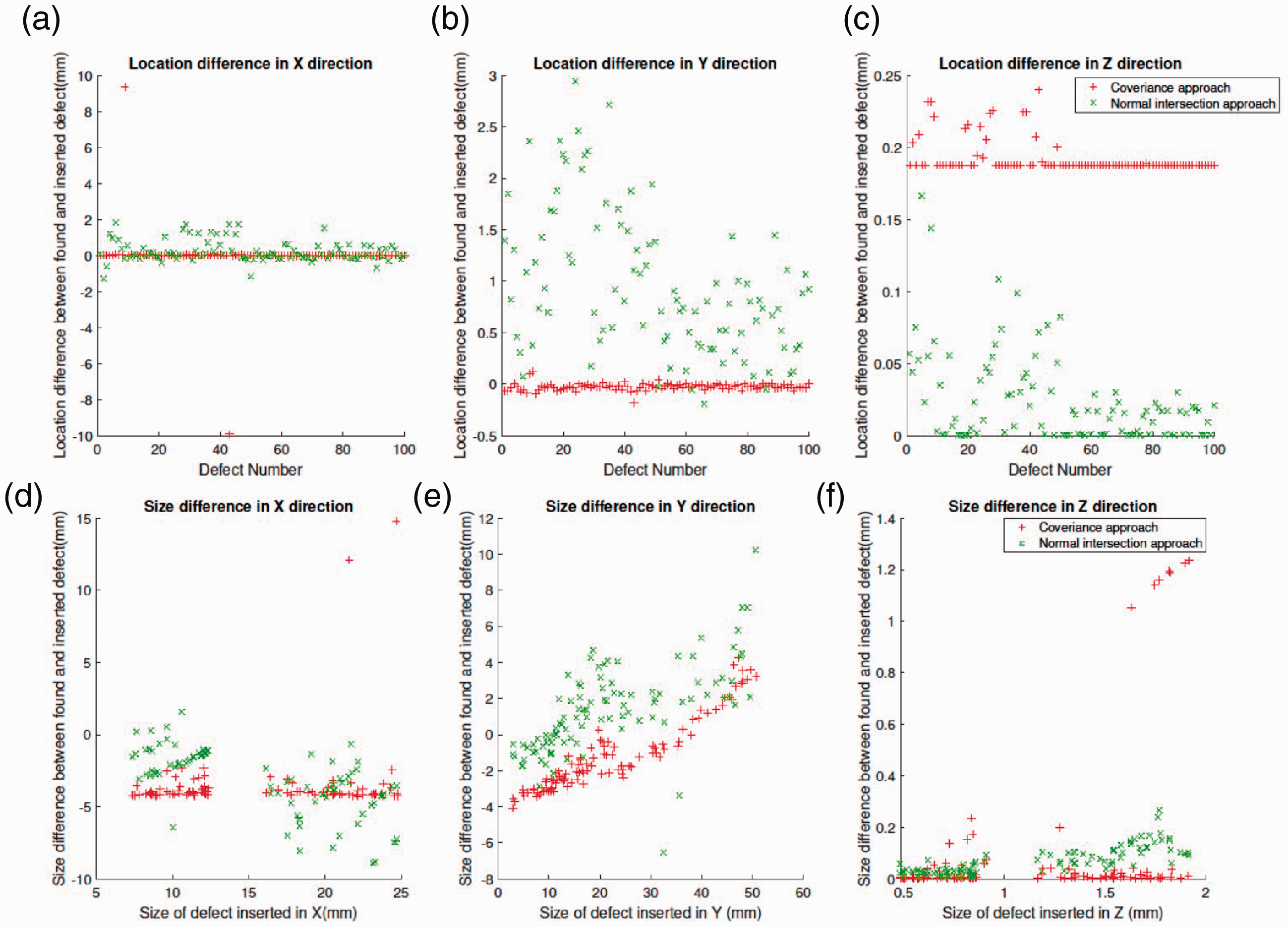
Plots of location error (a-c) against defect size and defect size error against defect size (d-f).

Table 1.

Table showing location (a) and size (b) mean error and standard deviation.

Covariance	X(mm)	Y(mm)	Z(mm)
(a) Location error
Mean error	0.004	–0.026	0.193
Standard deviation	1.370	0.035	0.012
Normal intersection	X(mm)	Y(mm)	Z(mm)
Mean error	–3.059	1.321	0.068
Standard deviation	0.594	0.693	0.031
(b) Size error
Mean error	–4.818	2.047	–0.001
Standard deviation	0.576	2.535	0.246
Normal intersection	X(mm)	Y(mm)	Z(mm)
Mean error	5.130	0.601	0.032
Standard deviation	3.392	2.392	0.168

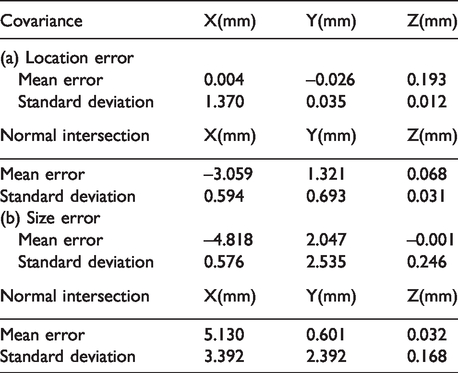
methods lie within 1.4 mm meaning that the accuracy of the location measurement for the Covariance method is in the X direction with an error of 0.004 mm ±1.37 mm while Normal Intersection method has an mean error in the X direction of –3.06 mm ±0.594 mm for a single standard deviation.

Figure 7 and Table 1(b) show the size difference between the measured defect and the inserted defect against its size. The three plots shown in Figure 7 are split based on their measurement direction. Figure 7 show that the Covariance approach identifies the defect more accurately and with a higher precision in both the X and Z direction with the inverse being true for the Y direction. Overall the both the Covariance Method and the Normal Intersection method show an accuracy value of –4.82 mm ±1.15 mm and 5.13 mm ±6.78 mm for the worst axes respectively. However, if a size constraint was placed on the algorithm these values could be reduced by eliminating some of the obvious outliers show in both the X and Z direction on Figure 7.

The simulation testing showed that both methods were good at locating and measuring a large range of squat defect sizes with various degrees of accuracy. However, the Covariance method showed a higher degree of accuracy compared to the Face Intersection method in locating the defect and would therefore be the preferred method when developing the rest of the rail repair system. The test results completed by previous authors such as Ye et al. and Xiong et al.^10,26 showed similar error however not enough testing was completed on specifically squat defects to make a statistically reliable comparison between the methods presented here and these papers.

Experimental testing

In order to verify the simulation model, physical testing was also completed on 4 machined defects. The defects were machined into a used piece of 60E2 rail. The 4 defects where made of various sizes along the rail and once machined, were measured using a Metris LK Ultra CMM. Three of the four defects were generated to be within the range of the simulated defects, while the smallest defect was created to test the limits of the algorithms. The depth of the defect was chosen as 0.2 mm nominally. This depth was chosen as Moldova et al. ⁴ states that a squat defect can be as small as 0.05 mm in depth, although other authors such as the ones mentioned in ‘Simulation of scanner data’ section state that a squat defect may be much larger than this. The measured defect sizes can be seen in Table 2 with Figure 8 showing the defects being scanned by the robotic arm. Figure 8 also shows the robotic test set- up as described in ‘Equipment used’ section. The scanning of the part was completed at 50 Hz with a robot TCP speed of approximately 5 mm/s

Table 2.

Table showing the size of machined defects as measured by the CMM.

	Width X (mm)	Length Y (mm)	Depth Z (mm)
Defect 1	4.082	7.100	0.289
Defect 2	9.551	15.053	1.030
Defect 3	12.515	17.720	1.551
Defect 4	15.414	22.5	2.871

Figure 8.

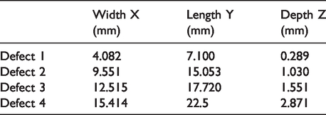
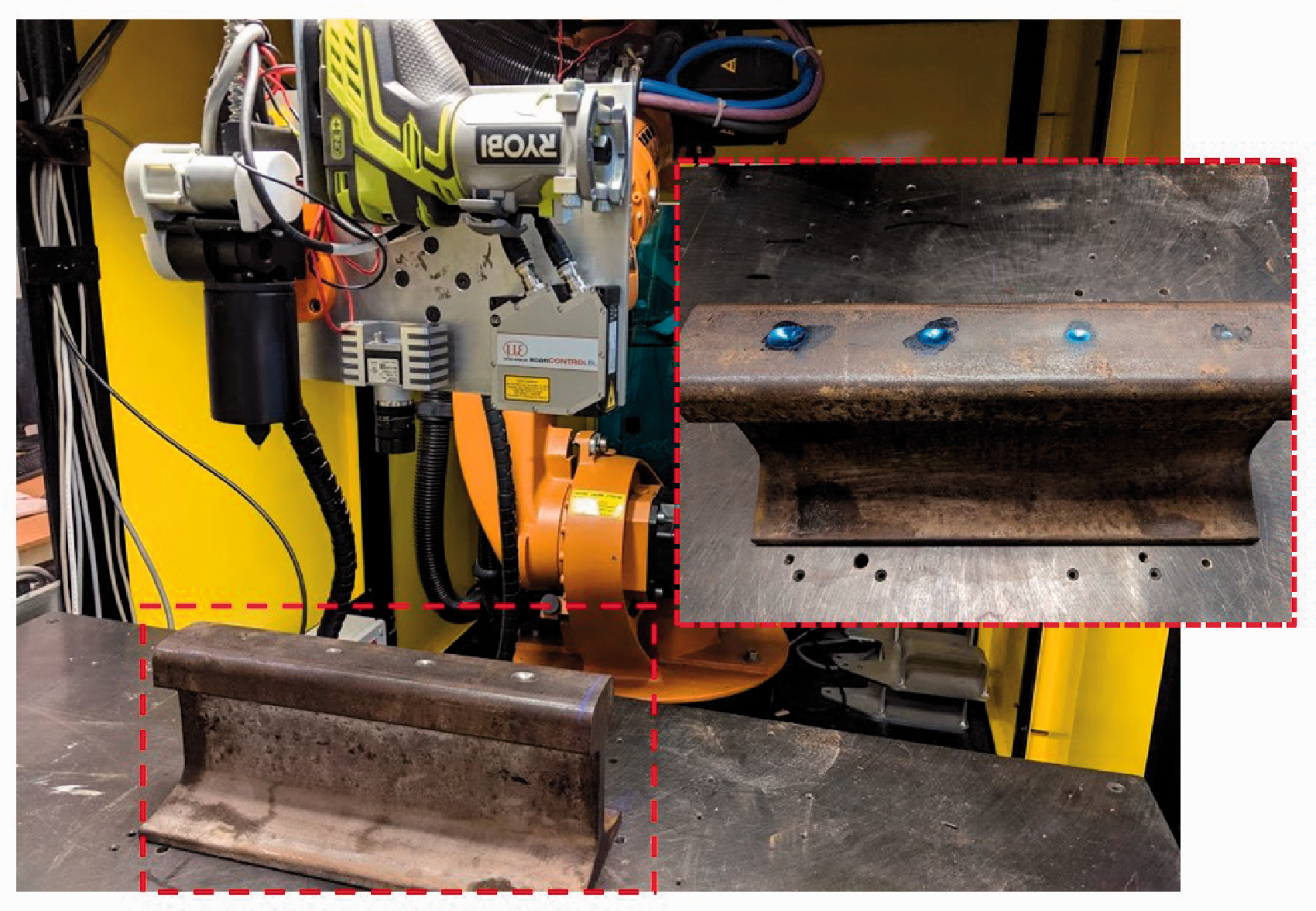
Image of rail with defects machined into it.

Experimental results

Once scanned the points were transformed to the robots base co-ordinate system in order to generate a 3 D profile of the defects. The 3 D generated point cloud of the scans can be seen in Figure 9 and the results of the size error can be seen in Figure 10. Although 4 defects have been inserted into the rail only three of the defects could be identified using the Covariance method while all the defects could be identified by the Normal Intersection method. The defect which could not be identified by the Covariance method was the smallest defect, labelled defect 1 in Table 2 and Figure 9. Due to the depth of the defect it was difficult for the algorithms to distinguish from any minor imperfections from wear and use of the rail prior to the insertion of the known defects. This is made apparent in Figure 9 (Defect 1).

Figure 9.

Plot of scanned defects.

Figure 10.

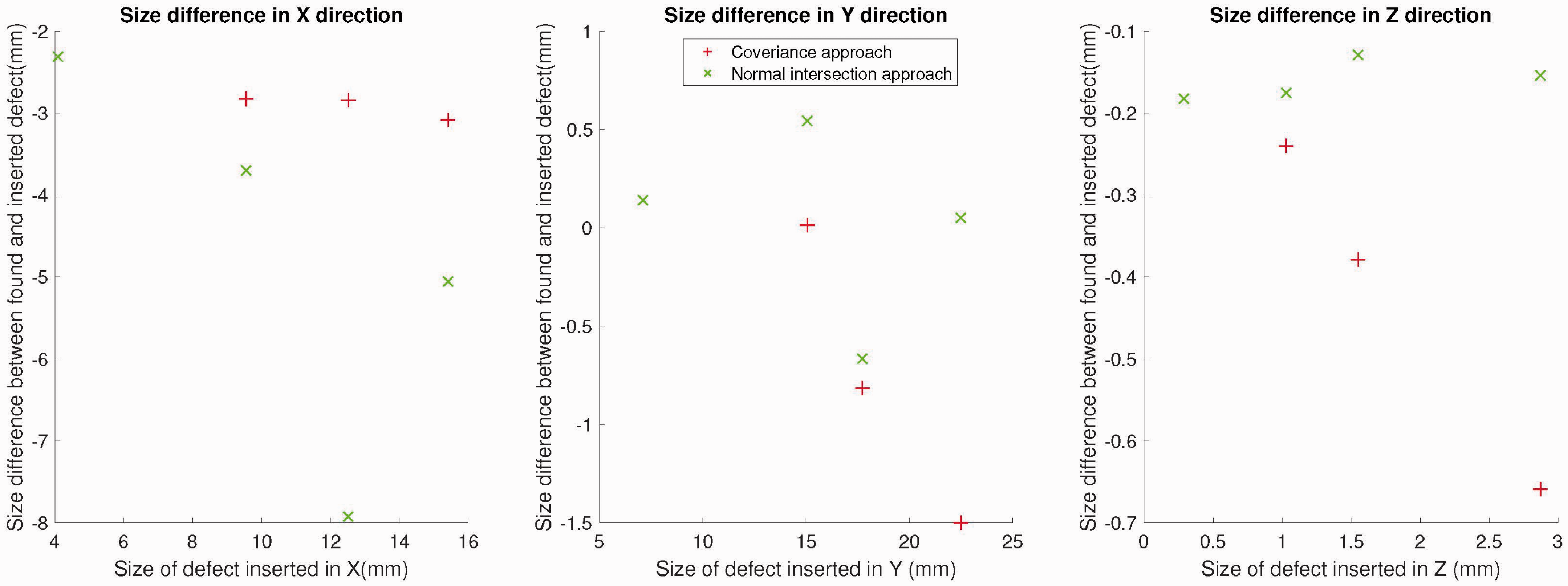
Experimental size error results.

which shows deviation from the curvature of the rail. This deviation is essential for the covariance method to work, as it requires a strong change in data trend between neighbourhoods.

The results of the other three defects which were found by both algorithms show a similar error to the simulation results with the covariance method showing a higher accuracy compared to the normal intersection method in all axes. Using the graphs shown in Figure 7 (d) to (f) and comparing the size error results shown in 10, the comparison shows that the error found in the simulated results strongly resembles the error found on the real component for both the Covariance and Normal intersection method. This is made apparent particularly with the same spike in error being shown in the Covariance method and in the simulation data when attempting to find a defect with a depth of greater than 2 mm. This correlation between the simulation and experimental data shows that the simulated data is a very good representation of the experimental results and thus could be used for any future testing or development of the detection systems.

Conclusion

This paper has presented a novel outline for a rail repair system. The methodology that has been outlined in this papers includes sub dividing this repair system into its three main constituents, including a defect identification system, a deposition system and finally a material removal system. The first stage of the system, a defect detection system, has been developed with two defect detection algorithms developed. Although previous work has been done in this area, to the authors knowledge there are no algorithms which use a laser line scanner or similar 3 D scanning system which does not require a region of interest to be identified first. The defect detection algorithms developed within this paper, although variations of algorithms already developed within literature, the work completed on these defect detection algorithms has allowed for the removal of the region of interest previously required. The work completed has also extensively tested these algorithms on a wide variety of representative squat defects thus testing the algorithms on a range of defect sizes and location. Finally both algorithms were verified on experimentally inserted defects.

To verify that the detection algorithms worked on a variety of defect sizes, they were tested against 100 simulated squat defects of various sizes. These squat defects were generated from the British Standard. Although this standard us specifically for for ABA measurement of squat defects, in principal there is no reason why this model could not be used to detect squat defects using other detection methods such as laser line scanning. This size range for the generated defects were taken from various sources within literature in order to cover the wide range of defect sizes which can occur. Both detection algorithms showed that they could identify the location and size of the squat defect with a few mm in the all axes. However, the results shown in ‘Simulation results’ section show that the Covariance method has a better accuracy at identifying the location of the squat defect. For the final repair system it could be argued that the location of the defect is more important that the size as removing more material than required is not as crucial as removing the material in the correct location. Therefore, moving forward with the development of the repair system the Covariance method would be used.

Further development of the repair system described in ‘Repair system architecture’ section and in Figure 4 will continue with the development of a defect removal system and a material deposition system. Once these two systems have been development and tested individually a final control system combining the defect detection system described in this paper and the two further systems can be joined into a single rail repair process. Finally, the future of this system would ultimately depend on the adoption of the system to the in house repair companies, and therefore for the system to operate would require the legislation to allow it do so. This adoption period could be reduced by adhering to as much of the current standards as possible.