Sage Journals: Discover world-class research

Abstract

A new method for supporting ground vehicle wind tunnel models is proposed. The technique employs a centrally mounted sting connecting the front face of the vehicle, adjacent to the floor, to a fixed point further upstream. Experiments were conducted on a 1/24^th-scale model, representative of a Heavy Goods Vehicle, at a width-based Reynolds number of 2.3 × 10⁵, with detailed comparisons made to more established support methodologies. Changes to mean drag coefficients, base pressures and wake velocities are all evaluated and assessed from both time-independent and time-dependent perspectives, with a particular focus within the wake region. Results show subtle changes in drag coefficient, together with discrete modifications to the flow-field, dependent on the method adopted. Subtle differences in base pressures and wake formation are also identified, with mounting the model upstream found to demonstrate retention of many of the beneficial effects of other techniques without suffering their deficiencies. Overall, these results identify the upstream mounting methodology as a viable alternative to currently available and more well-established techniques used to facilitate wind tunnel aerodynamic interrogation.

Keywords

Upstream model mounting front sting model support wind tunnel testing moving ground road vehicle

Introduction

Wind tunnel testing is a key tool used in road vehicle aerodynamic design to both assess and improve critical performance metrics. These vehicles emit more than 110 million tonnes of CO₂ into the atmosphere annually within the UK¹ and an urgent need exists to reduce their impact on the environment. Essential to these activities is the highest possible test fidelity, replicating, most holistically, realistic flow conditions.

The provision of moving air over a stationary model, typical to most wind tunnel testing, requires some form of mounting support. While the main aim of these structures is to hold the model, their presence often acts to increase measurement uncertainty in ways that remain difficult to quantify and challenging to predict.^2–6 Among the most common effects are changes to the surrounding flow-field, such as those occurring at the support-model junction.³ Simpson⁷ studied such junction flows between planar surfaces and streamlined obstructions, and showed the stagnation at the obstruction’s leading edge to provoke the upstream surface boundary layer to separate, resulting in the generation of horseshoe vortices, which propagate downstream. These vortices are typically small, less than the boundary layer thickness, and their strength increases with the bluntness of the obstacle.⁷ A secondary separation may also occur at the obstacle’s trailing edge, with Hetherington,³ who investigated similar effects on various mounting configurations, noting a significant localised momentum wake deficit caused by the support. Streamlining and filleting were identified as two ways to minimise those influences,^3,7,8 however, the disturbed flow was shown to affect the normal model aerodynamics with increases in pressure and friction drag.³ A dependency on Reynolds number, yaw orientation and model configuration was also found.^2,9–11 Furthermore, Hetherington³ shows the total force on a mounted ground vehicle model to be larger than the sum of the individual components (model and supports). Separate measurements using dummy supports (not connected) are normally used to correct such inconsistencies,^3–5 but a combination of both experimental and computational methodologies to obtain similar estimates can also be used, as outlined by Zhang et al.⁶

Many different road vehicle mounting techniques have been developed over the years, with each tending to be most suitable for specific test conditions and goals. One of the most common concepts is to support the model from above.^8,10–16 This method typically employs an aerodynamically streamlined strut connected to an internally, or externally fixed, measurement balance. Importantly, this arrangement facilitates both full-width moving ground use as well as wheel rotation and, as such, remains popular within the motorsport industry, where accurate ground-effect aerodynamic representation is essential. Flow interference and contamination of downstream components however, can be a significant source of uncertainty.^17,18 Page et al.⁹ has reported changes in pressure coefficient of up to ΔCp = −0.1 on the model roof directly ahead and behind of a top strut, reflective of the localised junction flow forcing an upstream and downstream roof separation. Additional changes have been noted by Strachan et al.¹⁴ on an Ahmed body (25° backlight angle) with a significant velocity deficit (u* ≈ 0.95) extending up to one model length downstream of the model base, with Strachan et al.¹¹ also showing the wake of the top strut to increase the surface pressure in the backlight region, resulting in the generation of weaker (C-pillar) corner vortices and premature bursting of the separation bubble. Strachan et al.¹¹ also noted a local central increase in downwash, attributed to the generated strut-model horseshoe vortex. This mechanism also prevented normal boundary layer development downstream of the support. Additionally, similar variations were also reported by Hetherington³ on a passenger car model, with results also showing a reduction in vehicle drag using a rear deflector in the absence of the top strut and an increase with the strut being used. Further work¹⁰ highlights the magnitude of these effects on a hatchback model with up to 7.5% and 28.2% increases in drag and lift coefficients, respectively. Notchback, fastback and motorsport configurations were shown less susceptible, with changes limited to between 1% and 3%^3,4 and 5%¹⁰ for drag and lift, respectively. The primary source of such changes was shown by Hetherington and Sims-Williams¹⁰ to vary between model configurations, with the increase in drag for notchback vehicles originating largely from the junction flow, and for hatchbacks, the support wake and consequent interactions with downstream flow being the main contributor.

Similar effects exist for the side-oriented support setups. This method usually incorporates struts fixed to the wheel hubs,^8,10,19,20 with underbody^21–23 and chassis²⁴ fixtures also utilised. This technique also facilitates moving ground use and wheel rotation, and has been shown to be less detrimental to drag measurements.^3,8 Miao et al.⁴ reported drag coefficient increases limited to 2% on a notchback passenger car model with both fixed and moving ground use. For the hatchback configuration on a stationary ground, drag increased by 1.4%, with results using a moving ground found only marginally more significant (1.7%).⁴ Front and rear wheel side strut pair influences were also found non-additive, suggesting the presence of complicated interactions. Hetherington and Sims-Williams¹⁰ attributed this small influence on drag to the position of the side struts, being typically located in an already highly turbulent flow where the local effects, such as junction flow, are subsequently minimised. Nevertheless, low ride-height racing vehicle configurations, which remain sensitive to lift (and downforce), have reported lift coefficient increases of up to 8.3%.¹⁰ Notchback passenger car models likewise have shown similar changes of up to 4.1%.⁸ This configuration has also shown the front wheel strut pair to contribute less to the lift increase (1%) in comparison with the rear pair (2.4%), further highlighting non-additive influences.⁸ Miao et al.⁴ also reported variations to be dependent on ground simulation, resulting in overall lift and downforce increases with stationary and moving ground use, respectively. The effect on lift has been reported by Hetherington³ to originate from the wake of the side strut impinging on the vehicle’s sides and affecting underbody pressures, with no obvious changes at higher vehicle positions.^3,10 Likewise, more localised flow-field modifications with struts fixed to wheel hubs have been reported by Knowles et al.²⁵ with notable reductions in the areas of high turbulence within the wheel wakes, resulting in weakened diffusion and mixing further downstream. Wittmeier et al.⁵ suggested using thin lateral cable supports to reduce the local effects, but noted the inclusion remains more difficult to quantify.

Using the combination of side supports with a top strut has also been investigated.^{8–10,19,20,26} Normally, no contact between the wheels and the body exists for such configurations, with component forces determined individually. This combination is typically more complex, particularly when testing at yaw.⁹ Increases in drag and lift coefficients of up to 6.9% and 15.8%, respectively, have been observed on a hatchback model.¹⁰ Again, the effects of the combination were found non-additive (top and sides separately) for most vehicle configurations, highlighting the complexity of the interactions which occur under these conditions.³

Underbody support systems are also common, particularly in commercial vehicle testing.^27–32 This method tends to minimise impact on the surrounding flow-field, with the added advantage of limiting any adverse impact when testing at yaw.²⁸ However, this system effectively precludes use of a full-width moving ground, limiting practical applicability. Recent advances in multi-belt configurations^5,19,33–36 have since compensated somewhat for this deficiency, also allowing wheel rotation, however, such facilities tend to be much more complex to operate and maintain. Additionally, in such cases, the support struts are typically positioned in line with the wheels, making an assessment of this area particularly difficult.³⁷ Tortosa et al.³⁷ described a facility where this could be alleviated by means of shifting the longitudinal position of the restraint posts depending on need, however, limits exist, particularly for long vehicles.

Rear-mounted support configurations also exist and remain popular within the aerospace industry. These can however, produce many unfavourable effects, particularly when located close to aircraft control surfaces (horizontal tail, etc.), with significant alteration to local pressure distributions.^38–40 Rear-mounted ground vehicles can also be adversely affected in this way within the sensitive base wake, making true and accurate reproduction of the natural flow-field difficult to achieve. Mercker and Knape⁴¹ identified this effect on a passenger car model, with a rearward-mounted sting entering at an angle through the back window shown to reduce drag by up to 4%.⁴¹ Noting such deficiencies however, Page et al.⁹ does suggest horizontal rear stings can be advantageous from a time-averaged flow perspective.

Other more exotic mounting methods have also been used, however, remain largely outside mainstream use. Magnetic suspension or levitation systems started to appear over 50 years ago, with early examples including support of bullet-like rotating bodies.⁴² The advantage of this type of support is the capability to remove any support structure affecting the flow-field. More recently, Muscroft et al.⁴³ successfully employed a comparable system on a simplified body representative of a Formula One car. However, the inclusion of rotating wheels and/or a moving ground was not easily attainable, with this technique also suffering from high initial costs, significant inherent complexity and large power requirements.⁴⁴

Supporting the model at the front or upstream is another option. This methodology has been used in the past within the aerospace industry to test free-flight sub-scale aircraft models,⁴⁵ but appears largely overlooked for ground vehicle applications; this omission being perhaps a result of the expectation that any upstream disturbance may be detrimental to the natural evolution of the aerodynamics. In reality however, all mounting configurations suffer, to differing degrees, from this issue, and if this can be overcome or minimised, the concept may offer a promising alternative for ground vehicle experimental investigations. For such a configuration, full-width moving ground use with wheel rotation remains a possibility, as does unhindered access to the base wake; both allowing realistic and detailed interrogation of the most sensitive region on which primary performance metrics (such as drag) fundamentally depend. Such a support configuration could also be expected to minimise the flow interference at the rear (if positioned close enough to the ground) and thus, impart minimum impact on the aerodynamics. Likewise, any increase in solid model blockage from supporting the model could be minimised, providing the means for a more favourable environment for replication of true aerodynamic performance.

With these considerations, this work aims to evaluate the concept of a front or upstream-oriented mounting method applied to a generic ground vehicle test model to determine suitability for purpose. Direct comparisons from both time-independent and time-dependent perspectives are made against other more established support methodologies from the top or sides with a particular focus centred within the base wake. These established techniques were chosen primarily given their popularity within the field as well as the capability to facilitate full-width moving ground use and wheel rotation. All tests incorporate the use of a full-width moving belt and wheel rotation, with drag coefficients, base pressures and detailed hot-wire anemometry (HWA) wake measurements compared, evaluated and assessed.

Experimental setup and apparatus

Baseline model

Figure 1 presents the simplified 1/24^th-scale model used (width, W = 110 mm). This baseline, representative of a Heavy Goods Vehicle (HGV), includes a rounded front (tractor) profile based on the Ground Transportation System (GTS)²⁸ and neglects fine detail. The model is made from Perspex and Aluminium and consists of two main parts: a tractor and trailer bottom section, and a trailer. This design allows the trailer to ‘free-float’, making contact at three points: via a load cell and connecting rod at the front face, and two sliding links towards the rear. The tractor-trailer gap was chosen relatively small (0.13W) to minimise any possible development of significant unsteadiness unrelated to the base wake, contaminating load cell signal quality. The model contacts the ground with eight fully rotating aluminium wheels equipped with bearings and supported by steel axels. Fixed at the wind tunnel centreline (y* = 0), the model’s front face is positioned Δx* = 3.3 downstream of the leading edge of a front flow splitter.

Figure 1.

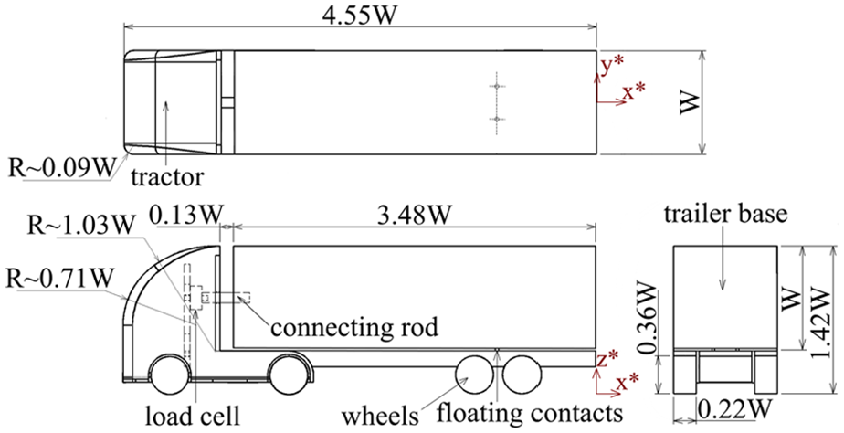
Schematic of baseline model.

Mounting configurations

The model was secured in the test section using three different techniques. The first used support struts from the model sides. For this purpose, two steel rods, of thickness = 0.03W, were used to replace the front and aft wheel axels, as indicated in Figure 2(a). The struts extended horizontally from the wheel hubs to each test section wall. This allowed fully rotatable wheels.

Figure 2.

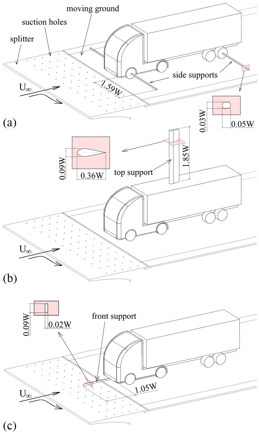
Schematic of the model installed in the test section via: (a) side supports, (b) top support and (c) front support.

The second supported the model from above. For this setup, an aerodynamically streamlined support strut affixed atop the trailer was used (Figure 2(b)). This extended through the wind tunnel roof (length = 1.85W) where it was mounted externally to a horizontal substructure. The same aerofoil profile used by Strachan et al.¹¹ was selected for this purpose. The thickness-to-chord ratio was 0.25 (chord = 0.36W), with the strut positioned at the model centreline, Δx* = 2.18 downstream of the tractor front face.

The front mounting configuration investigated is shown in Figure 2(c). An L-shaped metal support of thickness 0.02W was attached to the underside of the tractor, extending upstream by 1.05W. At this location, it was rigidly fixed to the test section floor. This design was chosen for two main reasons: (1) to minimise solid support-related blockage affecting the flow underneath the model and (2) to ensure sufficient structural stiffness to resist aerodynamic loading. The sting is also positioned close to the ground (0.01W), below the front stagnation position of the model, to better facilitate any disturbance being directed under the model, minimising its impact (Figure 2(c)). For all three configurations, during installation, the model was elevated (0.01W) before being fixed in place. This ensured the wheels only made light contact with the ground, minimising rolling resistance.

Wind tunnel

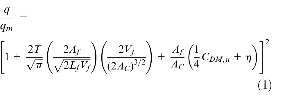
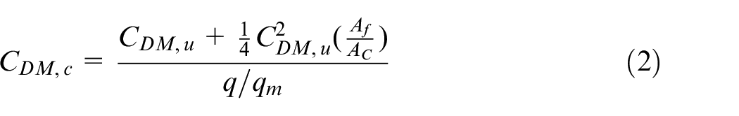
The experiments were conducted in an open-circuit wind tunnel with a closed test section measuring 1.3 m long, 0.46 m wide and 0.36 m high. The freestream velocity for all tests was U_∞ = 30 m/s, resulting in a width-based Reynolds number of Re_W = 2.3 × 10⁵. Freestream uniformity, turbulence intensity and heightwise velocity consistency at a central test section (empty) position are ±1%, 0.5% and ±1%, respectively. Based on the frontal areas of the model and support structures, the solid blockage ratios for the three configurations were 11.2% (top), 10.8% (side) and 10.0% (front); all considerably below the 15% limit suggested in SAE J1252.⁴⁶ All data was corrected for blockage using Mercker’s method,⁴⁷ with dynamic pressure and drag coefficient corrected by equations (1) and (2), respectively. This method was chosen based on its suitability for the test model chosen (sharper corners), facilitating some sensitivity to frontal separation.⁴⁸ As recommended by Cooper,⁴⁹ all data was corrected with η = 0.41.

\frac{q}{q_{m}} = {[1 + \frac{2 T}{\sqrt{π}} (\frac{2 A_{f}}{\sqrt{2 L_{f} V_{f}}}) (\frac{2 V_{f}}{{(2 A_{C})}^{3 / 2}}) + \frac{A_{f}}{A_{C}} (\frac{1}{4} C_{DM, u} + η)]}^{2}

(1)

C_{DM, c} = \frac{C_{DM, u} + \frac{1}{4} C_{DM, u}^{2} (\frac{A_{f}}{A_{C}})}{q / q_{m}}

(2)

The wind tunnel includes a centrally mounted moving belt, Δy* = 3.27 wide and Δx* = 7.5 long. The belt speed is matched to freestream velocity within ±1 m/s and monitored using LabVIEW software. Its motion precipitated wheel rotation. Suction is applied to the underside of the belt to prevent lifting during operation, with cooling water circulated through the floor to aid heat rejection. When operating, the freestream velocity profile is within 0.9 < u* < 1 a distance z* ≥ 0.045 above the floor, with a front splitter incorporating suction holes installed to further reduce boundary layer development (Figure 2).

Load measurements

The load cell used in all tests is a Model 31 single axis tension/compression load cell (full scale output of 44N) by RDP Electronics. The mounting position, load cell and rod used to connect the tractor and trailer are shown in Figure 1. This arrangement allowed measurement of drag of the ‘free-floating’ trailer (C_DT) for all three configurations. Total model drag (C_DM) was measured for the top mounting configuration using a Tedea Huntleigh compression load cell (full scale output of 196N) affixed directly to the top support strut and supported externally by the wind tunnel roof. For the top mounting system, trailer drag is determined from the difference between the two load cells.

Both load cells were calibrated in situ for a maximum load of up to 10N. To assess C_DT, eleven equally spaced calibration steps up to 1.2N were used, with a further 10 equal steps up to 10N for C_DM (top support only). These calibration ranges were chosen based on expectations. All points were sampled at 20 kHz for 40 s, with this process repeated three times to assess variability. Uncertainty estimates, encompassing overall repeatability, thermal drift and non-linearity, were less than ΔC_DM = ±0.018 (±10N range) and ΔC_DT = ±0.010 (±1.2N range).

The drag was sampled at up to 25 kHz for 20 s and averaged from up to four measurements. The initial ‘wind-off’ load measurement (moving ground on) was used for data correction as recommended in SAE J1252.⁴⁶ Additional measurements taken using a dummy top strut extending down to, but not touching the top of the trailer (2 mm separation), and with the model fixed by a rear-mounted support sting, were used to correct for top strut tare. No attempt was made to correct for the side strut tare, since only trailer drag alone is measured.

Prior to testing, the sensitivity of total model and trailer drag coefficients (C_DM and C_DT respectively) to Reynolds number was evaluated. These results are presented in Figure 3 with only a weak dependence evident for both C_DM and C_DT.

Figure 3.

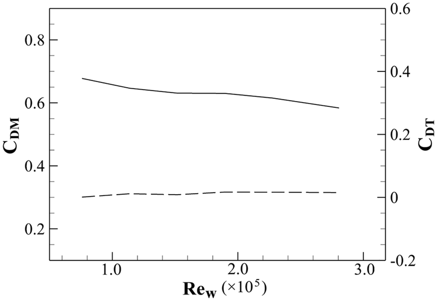
Variation of drag coefficient with Reynolds number; C_DM (solid), C_DT (dashed).

Hot-wire anemometry

The flow-field was assessed using hot-wire anemometry (HWA). A dual sensor x-wire probe was used in conjunction with an automated 3D traverse system (resolution 0.01 mm). The probe was calibrated in the velocity range from 0.5 to 40 m/s, with polynomial coefficients determined by 20-point curve-fitting. A separate directional calibration, with the probe axis varying between −40° and 40° (5° increments), was also performed to determine the probe yaw factors. The probe overheat ratio was set to 0.8,⁵⁰ with all results corrected for ambient temperature changes. The maximum velocity uncertainty within the obtained range was less than ±1 m/s (Δu* = ±0.033).

HWA was chosen as the main analysis tool for its ability to provide high frequency spectral content to small spatial resolution at reasonable cost. This technique does not allow accurate determination of direction within reversed flow regions (recirculating wake, etc.), however, general inference in terms of velocity magnitude and spectral content is offered where appropriate.^12,51–53 Outside these areas, all data lie well within the limits (u_rms* < 0.3, u_rms/u < 0.5) specified by Chandrsuda and Bradshaw.⁵⁴

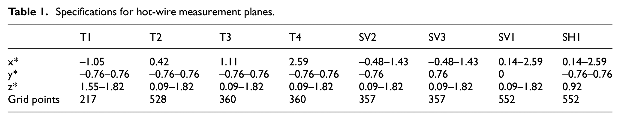
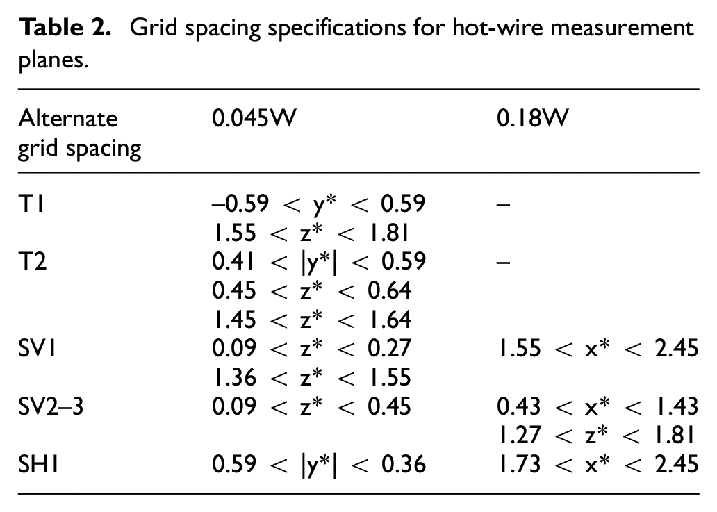
Measurements were taken at eight different planes: four transverse planes (T1–4), three streamwise vertical planes (SV1–3) and one streamwise horizontal plane (SH1). The size and position of these planes are described in Figure 4(a) and Table 1. Planes T1 and SV2–3 were included to capture the flow-field directly downstream of the top and side support struts, respectively. Measurement points were selected equally spaced throughout (0.091W), however, a finer resolution (0.045W) was selected in areas of specific interest (i.e. separated shear layers, etc.). Grid spacing was also increased (0.18W) in other areas to reduce test duration where possible. These point distributions are summarised in Table 2. To minimise the risk of probe damage, a lower limit of z* = 0.091 was set for all planes with sensor wires located Δx* = 0.73 upstream of the probe vertical support strut. All hot-wire data was sampled at up to 25 kHz for 20 s. The results are presented interpolated by a factor of two (using Gaussian process regression) to enhance feature detail.

Figure 4.

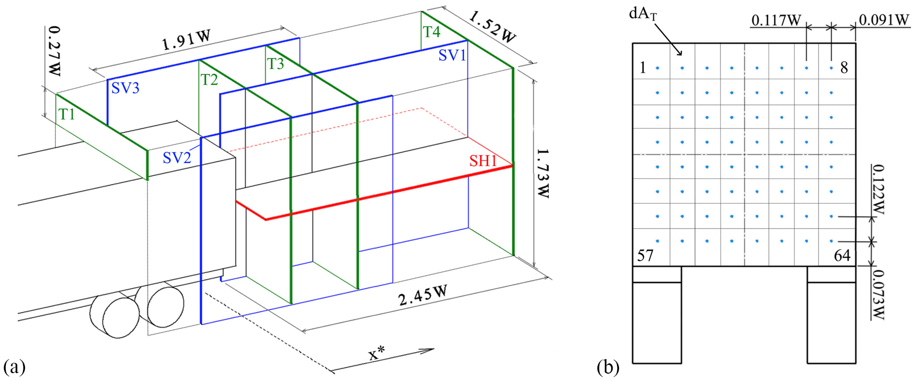
Schematics of measurement positions: (a) HWA planes and (b) base pressure.

Table 1.

Specifications for hot-wire measurement planes.

	T1	T2	T3	T4	SV2	SV3	SV1	SH1
x*	–1.05	0.42	1.11	2.59	–0.48–1.43	–0.48–1.43	0.14–2.59	0.14–2.59
y*	–0.76–0.76	–0.76–0.76	–0.76–0.76	–0.76–0.76	–0.76	0.76	0	–0.76–0.76
z*	1.55–1.82	0.09–1.82	0.09–1.82	0.09–1.82	0.09–1.82	0.09–1.82	0.09–1.82	0.92
Grid points	217	528	360	360	357	357	552	552

Table 2.

Grid spacing specifications for hot-wire measurement planes.

Alternate grid spacing	0.045W	0.18W
T1	–0.59 < y* < 0.59	–
T1	1.55 < z* < 1.81	–
T2	0.41 < \|y*\| < 0.59	–
	0.45 < z* < 0.64
	1.45 < z* < 1.64
SV1	0.09 < z* < 0.27	1.55 < x* < 2.45
SV1	1.36 < z* < 1.55	1.55 < x* < 2.45
SV2–3	0.09 < z* < 0.45	0.43 < x* < 1.43
SV2–3	0.09 < z* < 0.45	1.27 < z* < 1.81
SH1	0.59 < \|y*\| < 0.36	1.73 < x* < 2.45

Base pressure measurements

A Scanivalve MPS-4264 was used to measure the base surface pressures at 64 equally spaced positions (Figure 4(b)) using 0.8 mm surface holes via 90 mm long silicon tubing (1 mm ID). The frequency response characteristics of the connecting tubing were assessed against a Bruel and Kiaer 4133 laboratory standard microphone up to 400 Hz. All presented results are corrected for these variations using a method similar to that of Sims-Williams and Dominy.⁵⁵

The sampled data was transmitted to a PC using a custom-built wireless communication system fitted inside the trailer. The system used a battery-powered Belkin N100 wireless access point to relay 60 s of data at a rate of 800 Hz, providing 48,000 samples for subsequent post-processing. A separate connecting pneumatic tube, channelled out the trailer and test section, was used to measure the reference static pressure at a port located on the side of the wind tunnel directly adjacent to the trailer base. The pressure measurements were made independent of hot-wire tests, with all results averaged over three separate runs. The maximum pressure coefficient uncertainty is less than ΔCp = ±0.006.

Results and discussion

Drag coefficients

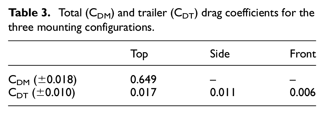
Drag coefficients for all three mounting configurations are presented in Table 3. Total drag of the model (C_DM) determined by the top configuration is C_DM ≈ 0.649. This is in general agreement to similar model configurations in other studies (C_DM ≈ 0.5,⁵⁶ C_DM ≈ 0.75,⁵⁷ C_DM ≈ 0.586,⁵⁸ C_DM ≈ 0.641⁵⁹). A small overall contribution of the trailer to total drag is characteristic for all three configurations. This is likely the result of the influence of the small tractor-trailer gap. In such a configuration, lower surface pressures are known to act on the trailer front, promoting reduced trailer-alone drag results.^60–62 Also shown in Table 3 is trailer drag being larger for the top mounting (C_DT ≈ 0.017) in comparison to the side (C_DT ≈ 0.011) and front (C_DT ≈ 0.006) setups. These changes are very subtle, with all lying within the experimental uncertainty (±0.010).

Table 3.

Total (C_DM) and trailer (C_DT) drag coefficients for the three mounting configurations.

	Top	Side	Front
C_DM (±0.018)	0.649	–	–
C_DT (±0.010)	0.017	0.011	0.006

Time-averaged base pressure

Figure 5(a) presents base pressure coefficient (Cp) distributions for all three configurations. Relative differences to the front-mounted configuration are also indicated for direct comparison. Overall, topologies indicate general similarities, with all showing a vertical symmetry and horizontal asymmetry. Maximum Cp is shown close to the top trailing edge, with magnitudes decreasing to a minimum at lower base locations. This topology is typical to this model type^28,63–67 and corresponds to regions dictated by the upper-recirculating flow impingement and lower wake vortex core proximity, respectively.^53,68,69 The former appears slightly more pronounced in Figure 5(a)(iii) (side), with Figure 5(a)(iv) indicating a localised increase of ΔCp ≈ 0.007 at z* ≈ 1.36 relative to Figure 5(a)(i). A similar comparison between Figure 5(a)(ii) and (a)(i) (top to front) is shown less localised and more offset (ΔCp ≈ 0.01), with all magnitudes lower for the former. This suggests two dissimilar mechanisms are responsible for these relative changes: the former being a shift in vertical wake balance, and the latter, a reduction in wake length. Results presented in Table 3 for C_DT support the second allegation. The implications of these observations are discussed further in the following section.

Figure 5.

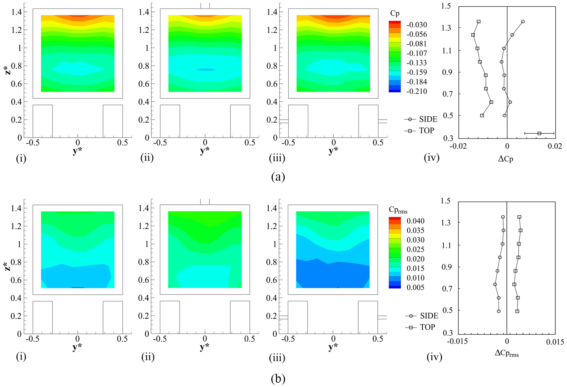
Time-averaged base pressure data: (a) Cp and (b) Cp_rms; (i) front, (ii) top, (iii) side and (iv) plots of differences top-front and side-front along the vertical centre.

Comparable root-mean-square (Cp_rms) results are presented in Figure 5(b). Again, a characteristic vertical symmetry and horizontal asymmetry is present, in general agreement with Castelain et al.⁵³ Figure 5(b)(ii) (top) is shown to produce the highest relative Cp_rms increase (ΔCp_rms ≈ 0.004 at z* ≈ 1.24 –Figure 5(b)(iv)), with Figure 5(b)(iii) (side) lower by a similar magnitude. In each case, all variations lie within experimental uncertainty indicating insensitivity to support configuration for these test conditions. Overall, the results presented in Figure 5 indicate the front mounting to have little influence on the base pressure distribution, showing trends in general agreement with the literature.^{28,53,63–69}

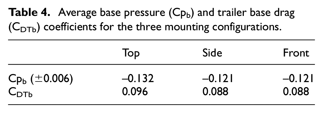
Results presented in Table 4 explore more global changes with average base pressure (Cp_b) and calculated trailer base drag (C_DTb) coefficients included for comparison. Both Cp_b and C_DTb are identical for the side and front mounting configurations, with the top support indicating a relative reduction in Cp_b and increase in C_DTb (9.1%); the latter in agreement with the trend identified in Table 3. Hetherington and Sims-Williams¹⁰ reported a similar trend with inclusion of a top strut, with a 7.5% increase in drag. No significant impact on drag from side struts was also identified in their work, with similar conclusions also drawn by Miao et al.⁴ The results presented here support these findings, and therefore, indicate the front-mounted setup does not materially impact mean drag production. The significance of the tractor-trailer gap at reducing trailer drag is also highlighted, with C_DTb contributing between 13.6% (front and side) and 14.8% (top) of total model drag (C_DM).

Table 4.

Average base pressure (Cp_b) and trailer base drag (C_DTb) coefficients for the three mounting configurations.

	Top	Side	Front
Cp_b (±0.006)	–0.132	–0.121	–0.121
C_DTb	0.096	0.088	0.088

Time-independent wake characteristics

Characteristics of the time-averaged wake are now explored. Initially, mean wake velocity magnitudes are considered. Detailed interrogation of each configuration is then presented, with the influence on time-dependent characteristics discussed thereafter.

Overall effects on the flow-field

Figure 6 presents the streamwise velocity (u*) contours in planes T2 and T4. In Figure 6(a), the wake is represented by lower velocity magnitudes directly downstream of the model profile. In each case, undisturbed freestream flow is shown to surround this area, except for remnants of the boundary layer close to the floor (|y*| > 0.5, z* ≈ 0.1). Within |y*| < 0.4, 0.45 < z* < 1.35, u* magnitudes are shown to decrease from trailer top to bottom, with minimum u* coinciding with minimum Cp values (Figure 5(a)), commensurate with the central location of the lower recirculating wake vortex core^53,66–68 and confirming the front sting does not fundamentally affect the mean structure of the base wake from this perspective. The wake is symmetric vertically, with closure attained by T4 for all three configurations (Figure 6(b)).

Figure 6.

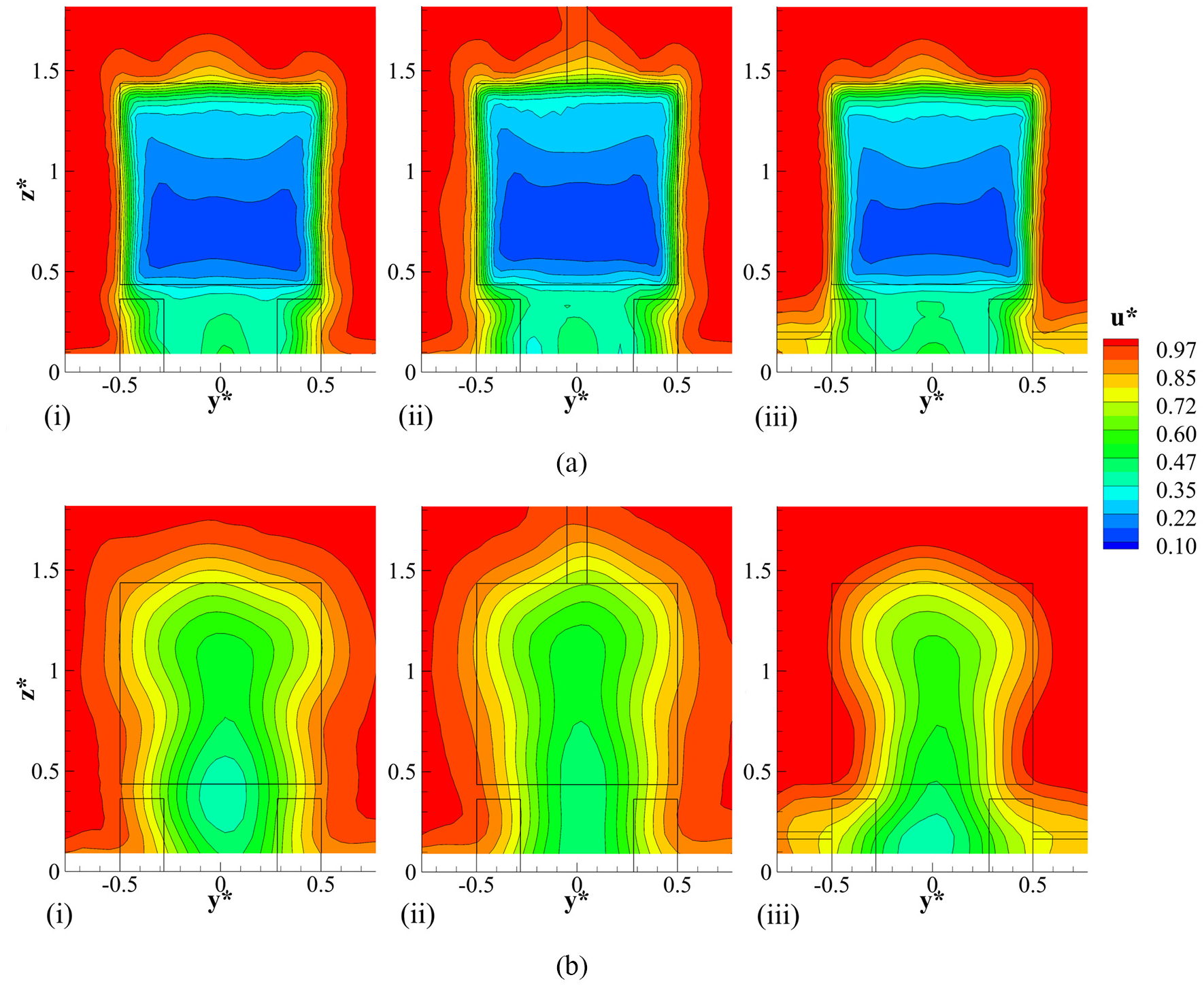
Contours of u* in T2 (a) and T4 (b) with: (i) front, (ii) top and (iii) side mounting.

Figure 6(a) shows u* topologies downstream of the base remain relatively unchanged for the front and top mounting methodologies, with the inclusion of side supports prompting a small reduction in size of lowest u* magnitudes (0.5 < z* < 0.8 - |y*| < 0.4). This suggests a subtle change in vertical wake balance has occurred, in agreement with Figure 5(a)(iv).⁶⁸ For the top mounting (Figure 6(a)(ii)), the influence of the support wake is captured (u* ≈ 0.95 at y* ≈ 0, z* ≈ 1.8) with a similar deficit (Δu* ≈ 0.05) and general topology to that reported by Strachan et al.¹¹ The influence of the side supports is also shown (Figure 6(a)(iii)– |y*| > 0.5, z* < 0.3) with regions of flow retardation up to Δu* ≈ 0.2 close to the floor, in general agreement with Hetherington.³ For the front mounting (Figure 6(a)(i)), similar effects are not observed, suggesting no comparable interference exists locally and showing the use of the front sting to eliminate the support wake influence typically reported for side³ and top^11,14 support setups.

The full impact of differing support strut configurations is further realised by considering results for plane T4 (Figure 6(b)). Both the top and front mounting configurations show only limited impact on mean wake development, each being approximately the same height and width (minimum u* located within |y*| < 0.2 at z* < 0.7). The side-mounted configuration (Figure 6(b)(iii)) however, appears to have a marked impact indicating a notable reduction in width above z*>0.5. This contraction would be expected to have both mean and unsteady implications on wake development, even though base pressure disparities appear marginal (Figure 5). As will be shown in the following sections, this change is precipitated by the increase in flow magnitudes around the model profile sides caused by the additional wake blockage. Given results appear very similar at T2 (Figure 6(a)), this data in particular, highlights the danger of making wide-ranging conclusions based on limited data sets.

To better quantify the relative changes identified in Figure 6, Figure 7 presents u* and ω* profiles at z* ≈ 0.5 (in T4) and y* ≈ 0 (SV1 – x* ≈ 0.14). For the side-mounted setup, the reduced wake width (Figure 6(b)(iii)) is clear in Figure 7(a). Using the bounded criterion Δu* ≈ −0.05 relative to freestream for comparison (indicated), a reduction from |y*| < 0.55 to |y*| < 0.48 is evident. The flow exiting the underbody (Figure 7(b) and (c)) also highlights a general insensitivity to mounting method at the vehicle centreline, with mean underbody mass flux (z* < 0.4 –Figure 7(b)) and relative upwash (z* < 0.4 –Figure 7(c)) all showing excellent agreement. From this perspective, these results suggest the front-mounted sting design adopted does not markedly affect the performance near the moving ground, similar to the top and side supports typically used for these applications.^3,4,9,11

Figure 7.

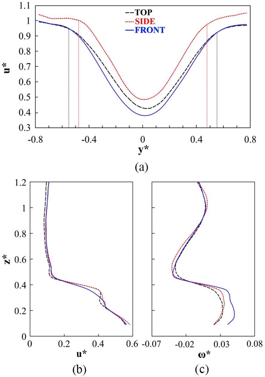
Velocity magnitude profiles: (a) u* in T4 at z* ≈ 0.5, (b) u* at x* ≈ 0.14 and y* ≈ 0 (SV1) and (c) ω* at x* ≈ 0.14 and y* ≈ 0 (SV1).

Impact on mean turbulence production within the wake

The contours of mean turbulent kinetic energy (K) presented in Figure 8 provide differences in turbulence production within T2. All configurations indicate elevated K principally surrounding the vehicle edges and directly behind the wheels. The front support (Figure 8(a)) indicates most intense K around the upper side and top edges of the model, as well as directly behind the wheels (0.3 < |y*| < 0.5, 0.9 < z* < 1.4 and 0.3 < |y*| < 0.5, 0.1 < z* < 0.35 respectively). Figure 8(b) (top) shows less intense K along the top edge (|y*| < 0.5, 1.3 < z* < 1.4) within the top separated shear layer. For this configuration, K production is also more intense behind the wheels, with a similar effect indicated in Figure 8(a). Magnitudes further dissipate within the region for Figure 8(c). Figure 8(d) highlights this disparity directly, as well as quantifying the significant difference (increase) to K production the side struts impart outside the region directly behind the model. Generally, these results (Figure 8(c) and (d)) agree with Knowles et al.,²⁵ showing reduced regions of high turbulence intensity within the wheel wake when using side struts, and show that the front sting imparts no similar influence, exhibiting a local topology largely comparable with the top strut.

Figure 8.

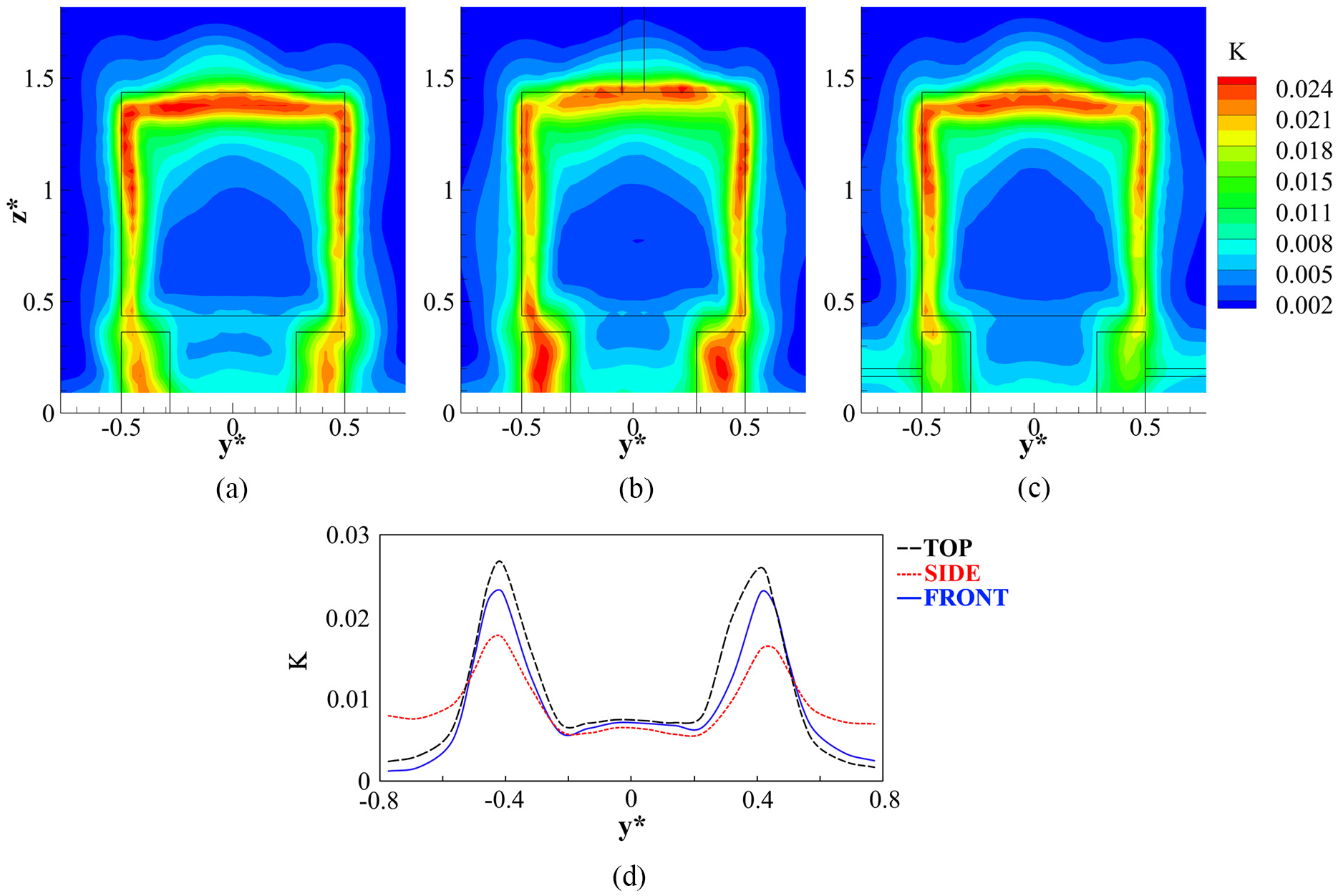
Average turbulent kinetic energy K in T2: (a) front, (b) top, (c) side mounting contours and (d) profiles at z* ≈ 0.18.

Localised influence of top support strut

To further assess the effects discussed more locally, Figure 9(a) presents u* variations at z* ≈ 1.8 within T1 for all three support configurations. Little change is shown between the side and front-mounted setups, consistent with the presence of undisturbed freestream flow. A similar trend exists for the top mounting configuration for |y*| > 0.1, with Δu* < 0.05 indicating only a limited influence exists within these areas. Between |y*| < 0.1 however, the top support strut produces the characteristic velocity deficit discussed previously. A similar corresponding change is shown in Figure 9(b) for u_rms*, indicating higher turbulence production (u_rms* ≈ 0.04) within the same area.

Figure 9.

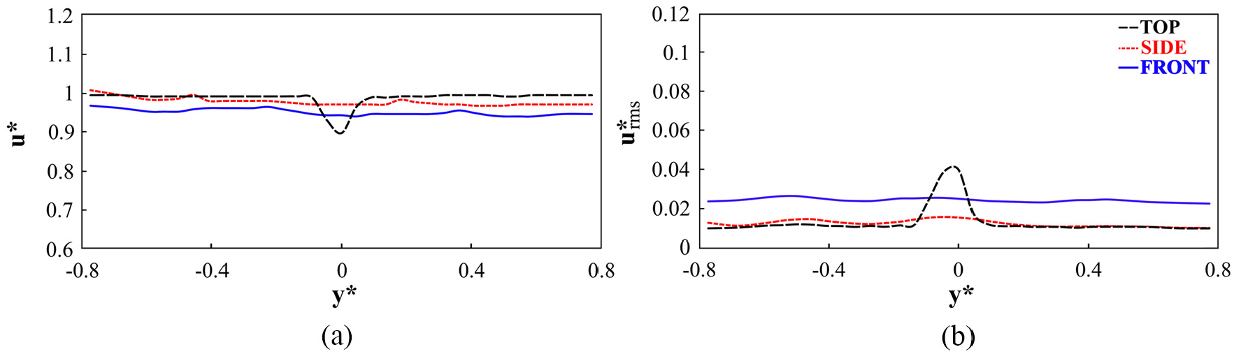
Spanwise profiles of: (a) u* and (b) u_rms*, at x* ≈ −1.05 (T1) and z* ≈ 1.8.

Further comparisons of K production at plane T1 are shown in Figure 10. For all configurations, increased K is evident in two primary areas: close to the trailer corners and coincident with the vehicle centreline. Topologies for the front (Figure 10(a)) and side (Figure 10(c)) configurations remain similar, with maximum K ≈ 0.011 and K ≈ 0.010, respectively (y* ≈ 0 –Figure 10(d)). Results behind the top strut however (Figure 10(b)), show marginally increased K over a greater width (Figure 10(d)) as the flow negotiates the obstruction caused by the strut.⁷ At z* ≈ 1.55 (Figure 10(d)), this configuration is also shown to produce a characteristic reduction in K (wake deficit) at the model centreline, with a relative increase also evident for z* > 1.7 (Figure 10(b)). The former agrees with suppression of the roof boundary layer downstream of the top strut suggested by Strachan et al.¹¹ and offers some support for the reduced turbulence levels within the top separated shear layer presented in Figure 8(b). Overall, the results within T1 for the front and side mounting setups show similar trends, with Hetherington³ also reporting the use of side struts to have little impact on the upper model portions.

Figure 10.

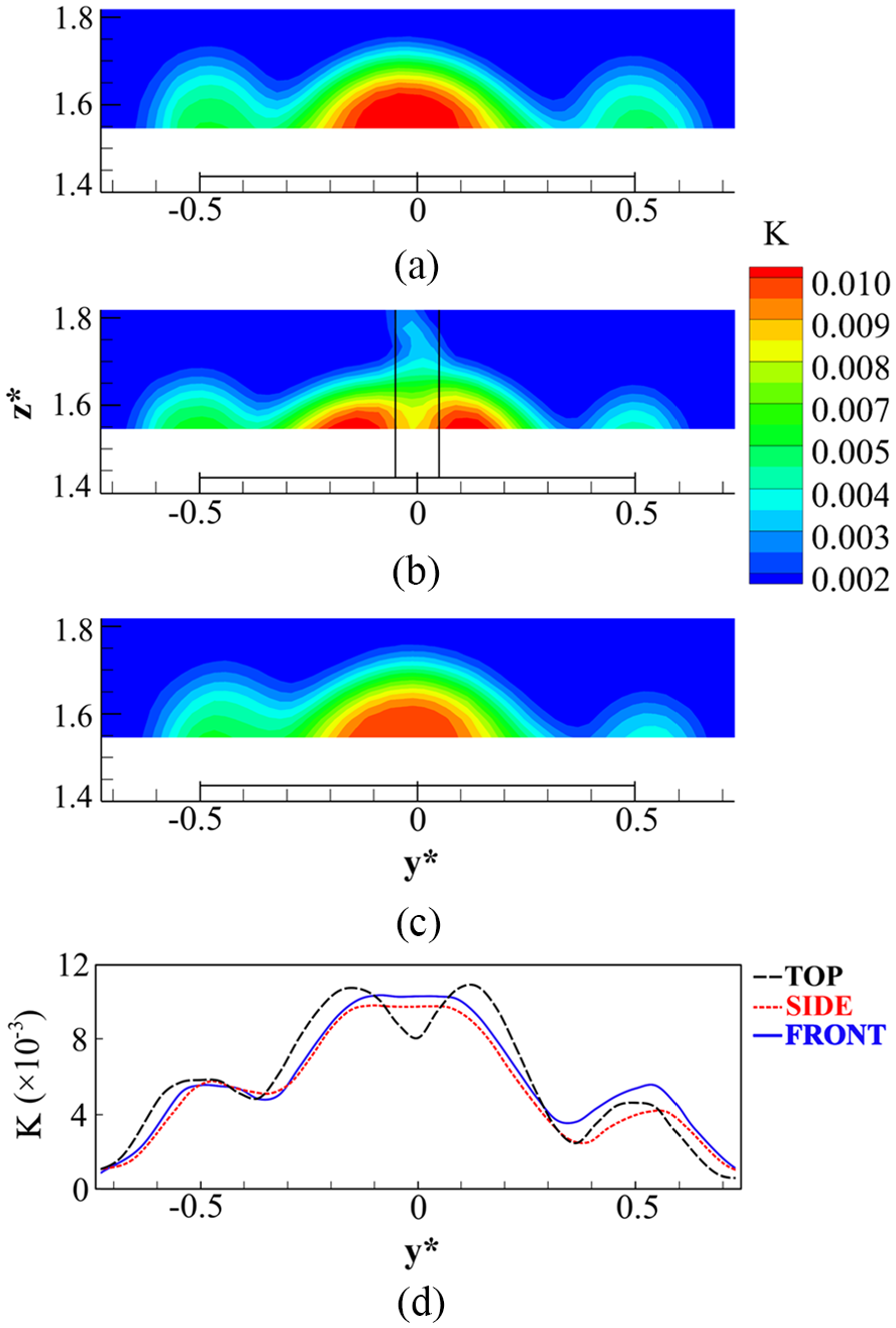
Average turbulent kinetic energy K in T1: (a) front, (b) top, (c) side and (d) profiles at z* ≈ 1.55.

Localised influence of side supports

The influence of the side supports is now considered (only left side included for brevity). Figure 11(a) presents the u* and u_rms* profiles at x* ≈ 0.25 for SV2. All three configurations show a near-uniform velocity profile with u* ≈ 1 consistent with undisturbed flow above z* ≈ 0.4 (Figure 11(a)(i)). Below z* ≈ 0.4, the side setup deviates markedly with a minimum of u* ≈ 0.76 at z* ≈ 0.2. This deficit represents the influence of wake generated by the strut, with the central axis coinciding with the location of minimum velocity magnitude. Further downstream (Figure 11(b)(i)), the side supports are also shown to markedly increase the local flow velocity adjacent to the model (z* > 0.6). This occurs from the additional blockage generated by their wake and reflects a change of up to Δu* ≈ 0.13 higher, with this effect precipitating the reduced wake width discussed previously (Figures 6(b) and 7(a)).

Figure 11.

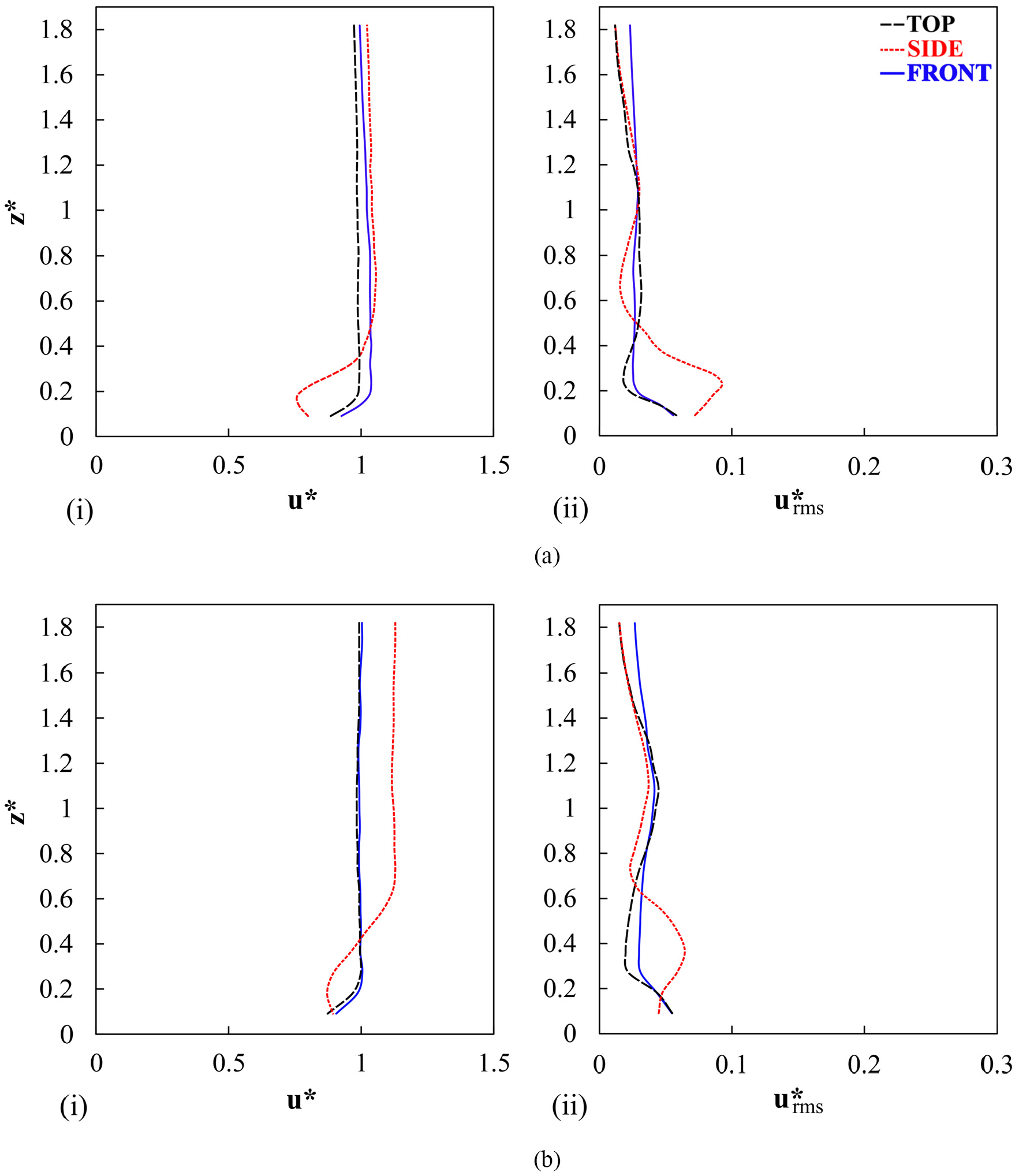
Profiles of u* (i) and u_rms* (ii) at: (a) x* ≈ 0.25 and y* ≈ −0.76 (SV2); (b) x* ≈ 2.59 and y* ≈ −0.76 (T4).

Results for u_rms* show similar deviations (Figure 11(a)(ii) and (b)(ii)). This metric indicates relative insensitivity to mounting method above z* ≈ 0.5 (u_rms* ≈ 0.025), but differing characteristics closer to the ground, particularly when using side supports. For this test case (Figure 11(a)(ii)), u_rms* increases markedly up to a maximum of u_rms* ≈ 0.093 (z* ≈ 0.22), signifying elevated turbulence production adjacent to the model wake. This region is shown to widen at T4 (Figure 11(b)(ii)) and reduce in magnitude to u_rms* ≈ 0.064, indicating the significant impact use of side supports can impart to the surrounding flow-field.

Figure 12(a) unlocks additional detail by presenting the Reynolds shear stress (u′ω′)* at SV2. The top and front mounting configurations show little variation except close to the ground, where traces of the boundary layer remain. Results are markedly different for the side-mounted configuration however, with the region 0.1 < z* < 0.5 indicating significant turbulent momentum flux typical of a separated wake. Unlike an axisymmetric wake however, these struts are dominated by significantly greater downward momentum due to the proximity of the ground. The vorticity results (Figure 12(b)) further highlight this effect, with Ω_Y magnitude being more intense and distributed above the strut than below. Downstream propagation is also more significant with a presence extending up to x* ≈ 1.

Figure 12.

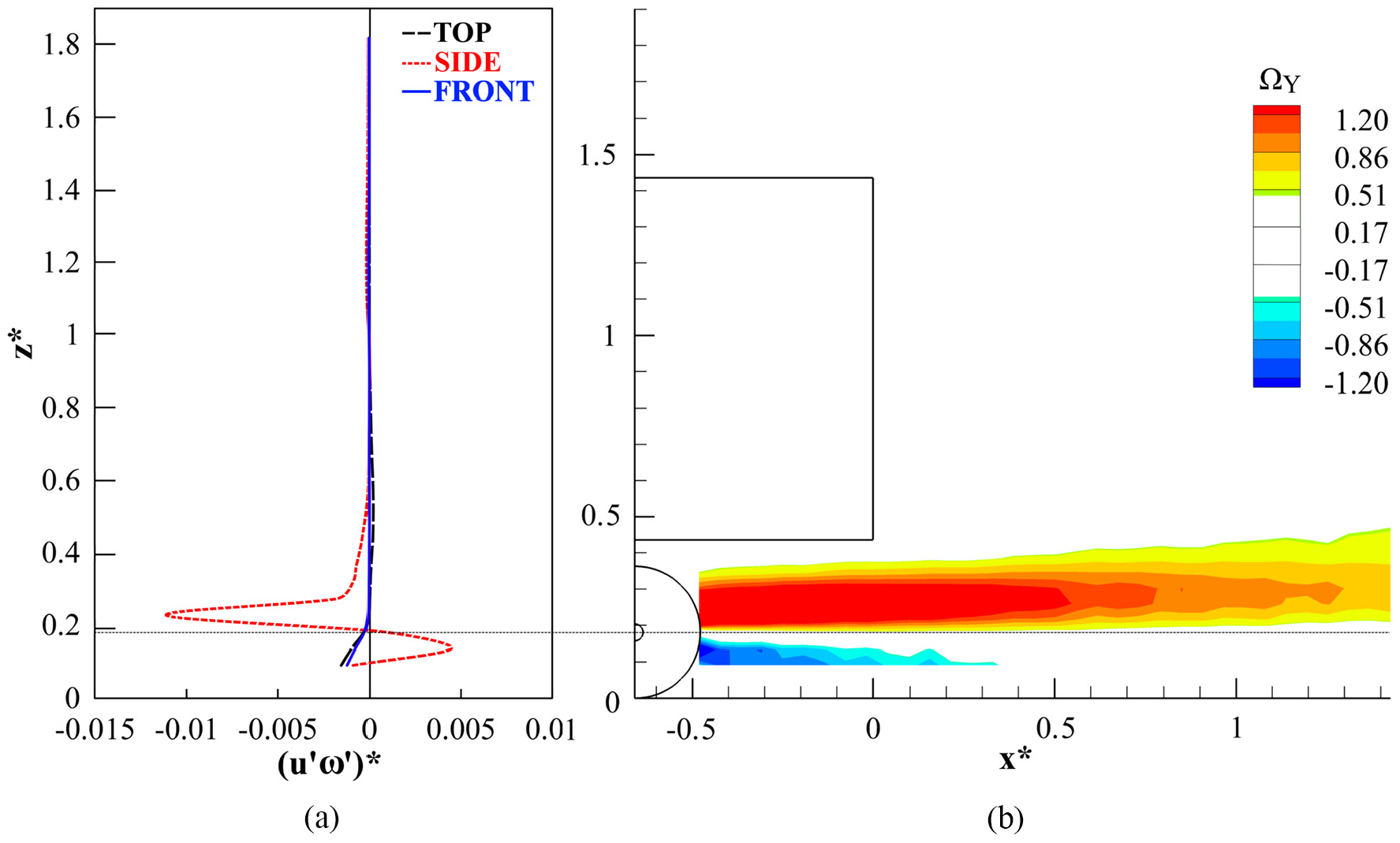
Side strut wake: (a) (u′ω′)* profiles at x* = −0.48 – SV2 and (b) Ω_Y contours for the side mounting configuration in SV2 (contours −0.5 < Ω_Y < 0.5 omitted).

This asymmetric flow over the side strut also produces secondary effects. Figure 13 presents the streamwise vorticity (Ω_X) contours downstream of this area at T2 (only left wheel data presented for brevity). For each instance, a common vortical structure (y* ≈ −0.4, z* ≈ 0.45) develops from the flow around the trailer bottom corner. Strength and size are similar in all cases (Δy* ≈ 0.1, Δz* ≈ 0.1 and Ω_Xmax ≈ 1.8), with comparisons between the front and top mounting suggesting similar characteristics. As shown in Figure 13(c) for the side-mounted setup, an additional structure develops closer to the ground, directly behind the wheel (y* ≈ −0.4, z* ≈ 0.15). This vortex is also indicated in Figure 13(a), albeit with a reduced magnitude, being even weaker in Figure 13(b). This decreasing trend stems from the increasing difference in flow magnitudes between the underbody (nominally invariant with mounting method –Figure 7(b)) and that adjacent to the outside of the wheel (Figure 6(a)(iii)). Lastly, the remnants of the vorticity produced over the side strut are also visible (Ω_X ≈ −0.55 at y* ≈ −0.6, z* ≈ 0.25 –Figure 13(c)). From this perspective, the similarities between the results for the top mounting, which typically affects upper-model portions,^3,11 and the front setup indicate no significant interference from the upstream sting on the flow near the ground.

Figure 13.

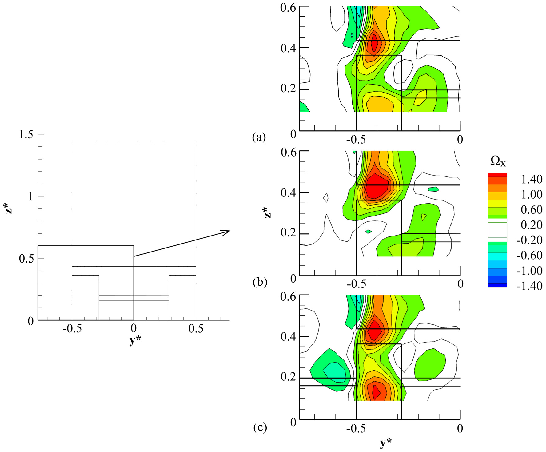
Streamwise vorticity (Ω_X) behind the left wheel in T2: (a) front, (b) top and (c) side mounting.

Time-dependent characteristics

Given results suggest the front-mounted support configuration is a viable alternative from a time-independent perspective, a comparison of time-dependent aspects is now considered. All wake velocity spectra presented are averaged from 39 time-segments (0.5 s duration), with a 50% overlap and bin widths of ΔSt_W ≈ 0.0052. Selected results are presented with offset magnitudes to aid interpretation.

Model wake dynamics

The general wake dynamics, including bubble pumping and shedding modes, for this model under identical test conditions have been previously described by Rejniak and Gatto.⁷⁰ The same peaks at St_W ≈ 0.107, corresponding to the bubble pumping characteristic frequency, are also evident here in the streamwise velocity spectra (E_u) within the separated side shear layers for all three configurations (Figure 14(a)). Comparisons to previous work show good agreement with Duell and George⁵¹– St_W ≈ 0.069, Khalighi et al.⁵²– St_W ≈ 0.098, Volpe et al.⁷¹– St_W ≈ 0.11, McArthur et al.³¹– St_W ≈ 0.08 and Pavia et al.⁶⁹– St_W ≈ 0.094. Wake oscillations, synonymous with lateral shedding, are also exposed within these results (E_v–Figure 14(b)), remaining largely insensitive to mounting method (St_W ≈ 0.212). Grandemange et al.,⁷² Volpe et al.⁷¹ and McArthur et al.³¹ all found similar lateral shedding characteristic frequencies. One possible exception may be the results using the side struts. As shown in Figures 6(a)(iii), 6(b)(iii) and 11, these struts produce a strong localised disturbance, which would be expected to impact this mechanism. Figure 14(c) also identifies a broader heightwise shedding mode at St_W ≈ 0.22. Unlike the results for the lateral shedding mode however, this mechanism appears largely unaffected by mounting configuration.

Figure 14.

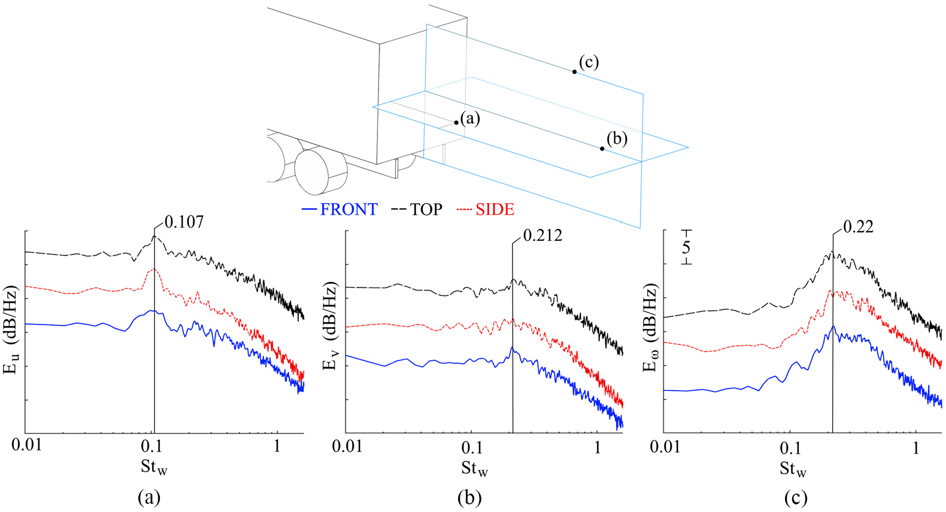
Velocity spectra in the wake: (a) E_u at x* = 0.64, y* = −0.36, z* = 0.92; (b) E_v at x* = 1.64, y* = 0, z* = 0.92; (c) E_ω at x* = 1.36, y* = 0, z* = 1.5 (relative offset of Δ5 dB/Hz).

Additional insight into these processes can be obtained through considering Proper Orthogonal Decomposition (POD)⁷³ of the base pressure signals. The first two modes with a combined energy content approximating half of the total are presented in Figure 15. In Figure 15(a) a near-uniform topology pervades for each configuration, confirming a near-global wake oscillation (bubble pumping mode). Comparing Figure 15(a)(i) (front) and (a)(ii) (top), near-identical energy levels are present, each being significantly higher relative to Figure 15(a)(iii) (side). This is a possible consequence of the influence the side struts impart to the base wake. The trends for the second mode are also shown in Figure 15(b). These results confirm the heightwise shedding mode identified in Figure 14(c), with energy content being approximately one-quarter that of the first mode (for top and front). In agreement with results presented in Figure 14(c), little variation exists between the mounting methods used. Overall, these results (Figures 14 and 15) further highlight that the front sting does not fundamentally affect the model wake dynamics, with typical processes and characteristic frequencies in good agreement with those reported in literature.^{31,51,52,69–71}

Figure 15.

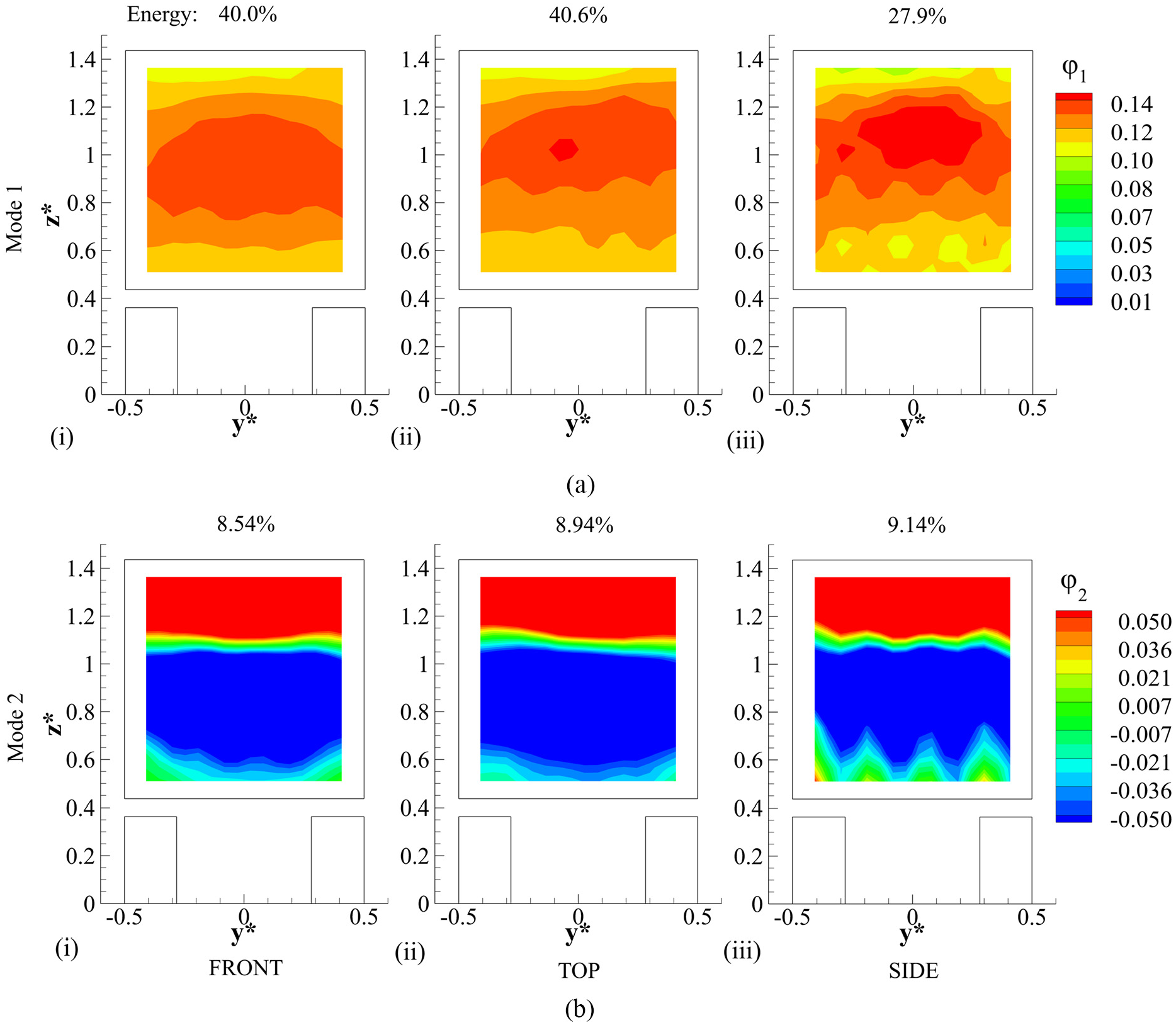
Fist two POD modes (Mode 1 – (a); Mode 2 – (b)) of the base pressure signals: (i) front, (ii) top and (iii) side mounting configurations.

Spectral comparisons

Finally, wake velocity spectra are compared at selected locations to assess the localised impact of the differing mounting methods. Figure 16 presents the lateral ((a)–(d)) and vertical ((d)–(f)) evolution at T1. At (a), streamwise velocity spectra (E_u) show little variation, indicating the flow remains insensitive to support configuration at this position. Further inboard at (b), a decrease in E_u ( ≈ 3–5 dB/Hz) is evident beyond St_W ≈ 0.1 for the top mounting, indicating a subtle reduction in high-frequency turbulence. The opposite is evident closer to the strut, with significantly higher E_u magnitudes at (c) and (d). A maximum increase (≈15–20 dB/Hz) is evident directly downstream of the strut centre at (d), confirming the top support wake as a source of localised turbulence at this distance away from the trailer roof, in agreement with Figure 10. Moving towards the top surface of the trailer however, the heightwise evolution of E_u (Figure 16) indicates relative reductions in magnitudes for the top-mounted setup at (e), with this trend persisting to lower positions ((f)), albeit to a lesser degree (≈2.5 dB/Hz reduction at St_W < 0.4). These results agree with Strachan et al.,¹¹ who note a suppressed boundary layer over the roof downstream of an overhead strut, and are consistent with the K results presented in Figure 10.

Figure 16.

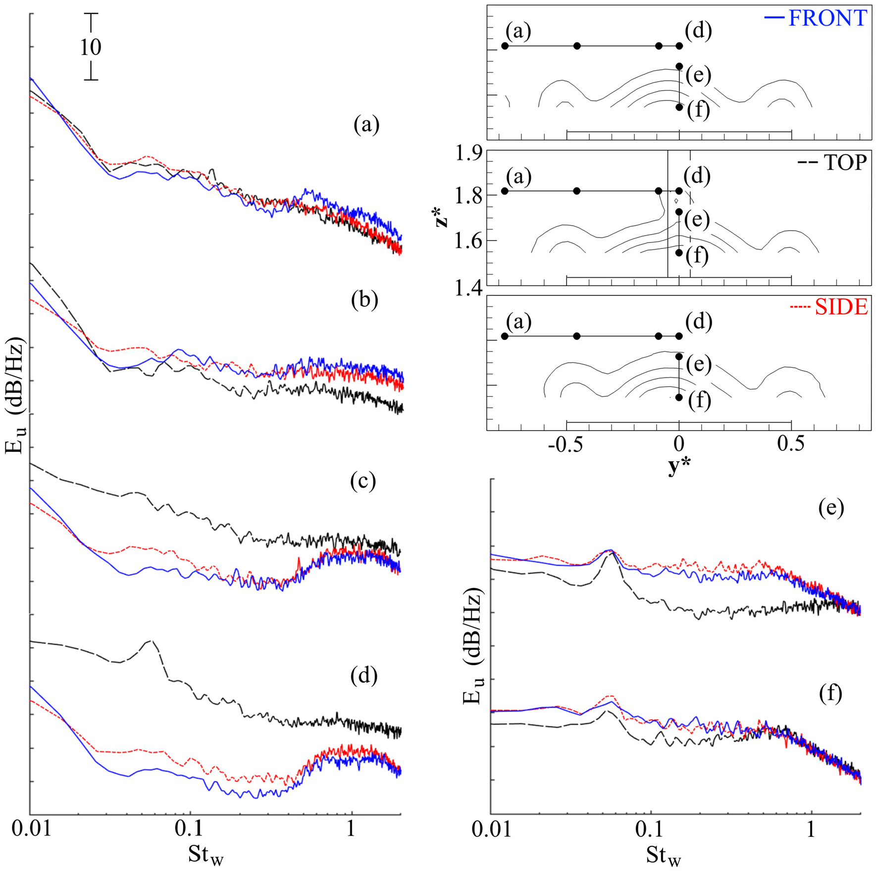
Selected velocity spectra (E_u) for T1 along −0.76 < y* < 0 at z* ≈ 1.82 and 1.55 < z* < 1.73 at y* ≈ 0.

The impact of the top strut is also assessed further downstream. Figure 17 presents the vertical evolution ((a)–(c)) of E_u at two different streamwise locations (I and II). At I, broad peaks centred around St_W ≈ 0.2 are discernible for all configurations at locations (a) and (c), corresponding to the heightwise shedding identified in Figure 14(c). At (a), the increase in magnitudes (up to 10 dB/Hz) below St_W ≈ 0.4 remains for the top-mounted configuration. Comparisons to position (d) in Figure 16 show the wake emanating from the strut persists further downstream. Moving downward through (b), this influence weakens, with no appreciable effect at (c). Further downstream at II (Figure 17), the impact of the top strut is no longer observable, with near-identical spectra between all configurations at all vertical positions ((a)–(c)). One exception is evident in the spectra of the front-mounted model at (a), showing magnitude reductions at lower frequencies relative to the other two setups, reflective of less intense turbulence within the freestream flow. Overall, general similarities between the side and front setups from this perspective confirm low levels of interference exist locally for both.³

Figure 17.

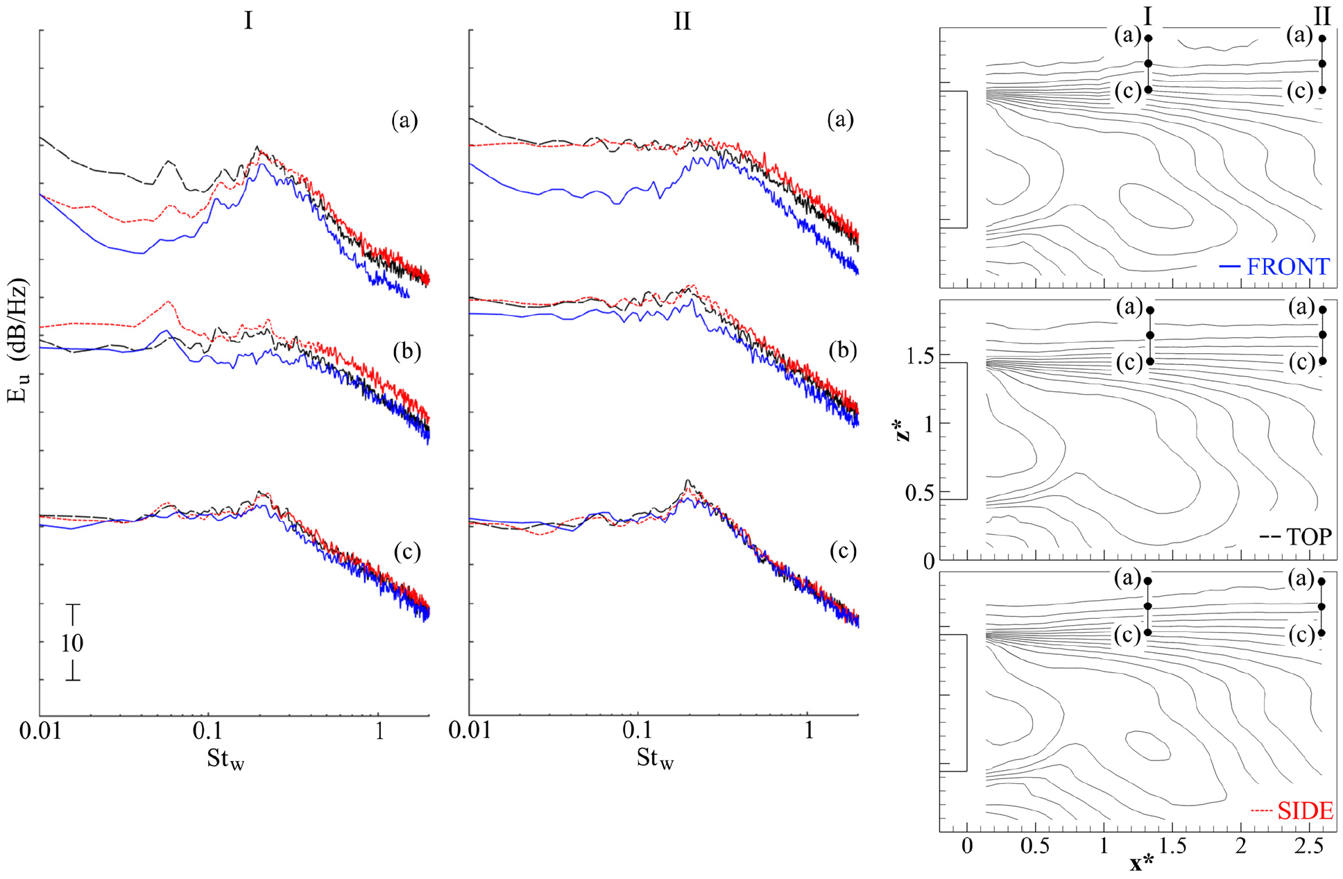
Selected velocity spectra (E_u) for SV1 along 1.45 < z* < 1.82 at x* ≈ 1.32 (I) and x* ≈ 2.59 (II).

The spectral characteristics of the side strut wake are evidenced in plane SV2, with E_u presented in Figure 18. Positions (a)–(e) show strong heightwise variations close to the strut, with positions (f)–(j) located further downstream. At position (a), closest to the ground, E_u show similar characteristics, with minor reductions in magnitude (≈1–5 dB/Hz) at the lowest frequencies (St_W < 0.1) for the side-mounted setup. A discrete peak is shown at St_W ≈ 0.82 for the front and side setups, corresponding to the wheel rotation frequency (St_W ≈ 0.80).⁷⁰ For the former, this peak persists up to position (d), with positions (a)–(c) also showing a related harmonic at St_W ≈ 1.64. For the side-mounted model at (b), magnitudes beyond St_W ≈ 0.1 show a relative increase of up to 10 dB/Hz. This increase is most significant at position (c) within the strut wake, with values up to 20 dB/Hz higher. These results confirm the influence of the side strut at producing substantial turbulence to the local flow-field. This influence is shown to persist vertically, with magnitudes at (d) increasing by 15 dB/Hz relative to the front-supported setup; the effect evident to z* ≈ 0.4. Additionally, the top-mounted model also shows higher magnitudes at this position (up to 10 dB/Hz relative to front), indicating additional streamwise unsteadiness. Higher E_u spectral energies for the top-mounted setup are also shown up to (e), with the magnitudes for the side support similar to those observed for the front-mounted configuration, suggesting a general flow insensitivity at this position.

Figure 18.

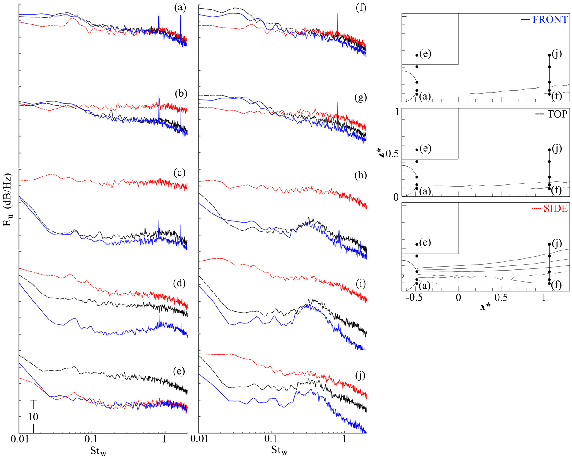
Selected velocity spectra (E_u) for SV2 along 0.09 < z* < 0.55 at x* ≈ −0.48 and x* ≈ 1.06.

Further downstream (Figure 18(f)–(j)), E_u trends close to the ground at (f) and (g) remain similar to (a) and (b), with the wheel rotation frequency (St_W ≈ 0.82)⁷⁰ again evident for the front mounting. At positions (h)–(j), the front and top mounting spectra capture broad peaks centred around St_W ≈ 0.4, with a subtle shift to a lower frequency for the former. At this position, this peak represents the lateral wheel wake shedding mode described by Rejniak and Gatto⁷⁰ with the use of a top strut, suggesting these characteristics are retained when using the front sting. The offset in magnitudes between these two configurations at (i) and (j) is still evident as in (d) and (e), albeit significantly lower (≈5 dB/Hz), suggesting the same effect of the top mounting seen upstream is weaker at these positions. With the model supported from the sides, the wheel wake signature appears completely inhibited by the overall increase in magnitudes ((h)–(j)), coherent with the results indicated in Figure 8. Higher unsteadiness for the side-mounted model is evident up to positions (h)–(j), confirming the side strut wake propagates downstream and upwards affecting the flow-field at higher positions, in agreement with Figures 6(a)(iii), 6(b)(iii), 11 and 12. A qualitative comparison to Figures 16 and 17 also reveals that the wake shed from the side strut has a broader, more significant, impact on the surrounding flow than the wake generated by the top strut. In this area, the overall trends for the front mounting are shown similar to the top-mounted model, suggesting no appreciable interference from the front support exists locally.

Conclusion

An experimental study comparing the effects of different wind tunnel model mounting techniques was conducted on a 1/24^th-scale model representative of a HGV at Re_W = 2.3 × 10⁵. With the focus on the flow-field around the vehicle base, a novel upstream support was assessed and compared to the more common techniques of mounting from the top and sides.

Evaluation of the recorded load data and base pressure showed the inclusion of the front sting to have little effect on the mean drag production. General base wake topologies were found similar for the top and front configurations, with a subtle relative change in vertical wake balance identified for the side setup. The local wakes generated by the top and side struts were clearly identified, with significant flow retardation accompanied by increases in turbulence production. The side struts were shown to alter the vorticity production around the rear wheel profile. Propagation of the wake of the side strut was also shown to affect the flow-field further downstream, with additional flow retardation produced close to the ground, resulting in velocity magnitude increases in the higher locations and subsequent reductions in wake width.

Analysis of the time-dependent aspects revealed no strongly defined oscillatory behaviour, with broader characteristic typical instead. The streamwise wake oscillation (bubble pumping) mode was found to dominate the wake dynamics, with the characteristic frequency insensitive to mounting configuration. With the side-mounted model however, the energy of bubble pumping was identified substantially weaker relative to mounting configurations from the front and top. The asymmetric shedding (flapping) from the vertical and horizontal base edges was also identified, largely insensitive to varying support methods, with the exception being the side setup exhibiting less defined lateral wake oscillation characteristics.

The top strut was found to increase turbulence production within the flow above the trailer and suppress fluctuations towards the roof surface boundary layer, with this influence weakening with downstream evolution. Similar, but more intense, increases in turbulence were also found behind the side struts. The wake generated by the side strut was also shown to propagate downstream and upward, with the overall increase in turbulence inhibiting wheel wake shedding characteristics.

Overall, results presented in this work show the front mounting configuration to exhibit the same or improved base flow-field characteristics in comparison with more conventional support techniques from the top and sides. No significant interference was found locally, along with only subtle effects identified from both mean and unsteady aerodynamic perspectives. These qualities highlight the possibility that this support methodology may represent a viable alternative for high fidelity road vehicle aerodynamic analysis.

Footnotes

Appendix

Declaration of conflicting interests

The author(s) declared no potential conflicts of interest with respect to the research, authorship, and/or publication of this article.

Funding

The author(s) disclosed receipt of the following financial support for the research, authorship, and/or publication of this article: This work was supported by the Engineering and Physical Sciences Research Council (Doctoral Training Program).

ORCID iDs

Aleksandra Anna Rejniak

Alvin Gatto

References

Department for Business Energy & Industrial Strategy. National Statistics, Final UK greenhouse gas emissions national statistics: 1990–2017, https://www.gov.uk/government/statistics/final-uk-greenhouse-gas-emissions-national-statistics-1990-2017 (2019, accessed 10 January 2020).

Wood

Reynolds number impact on commercial vehicle aerodynamics and performance. SAE Int J Commer Veh 2015; 8(2): 590–667.

Hetherington

Interference of supports used for ground vehicle wind tunnel testing. PhD Thesis, Durham University, UK, 2006.

Miao

Mack

Indinger

. Experimental and numerical investigation of automotive aerodynamics using DrivAer model. In: Proceedings of the ASME design engineering technical conference, Boston, Massachusetts, USA, 2–5 August 2015. New York: American Society of Mechanical Engineers (ASME).

Wittmeier

Michelbach

Wiedemann

, et al. The new interchangeable three-belt system in the IVK full-scale wind tunnel of University of Stuttgart: design and first results. SAE paper 2016-01-158, 2016.

Zhang

, et al. Test process and correction of automotive wind tunnel in Jilin University China. SAE paper 2013-01-1351, 2013.

Simpson

RL.

Junction flows. Annu Rev Fluid Mech 2001; 33: 415–433.

Hetherington

Sims-Williams

DB.

Wind tunnel model support strut interference. SAE paper 2004-01-0806, 2004.

Page

Winkler

Roberts

, et al. Recent upgrades to the Swift 8 ft × 9 ft rolling-road wind tunnel. SAE paper 2002-01-3341, 2002.

10.

Hetherington

Sims-Williams

DB.

Support strut interference effects on passenger and racing car wind tunnel models. SAE paper 2006-01-0565, 2006.

11.

Strachan

Knowles

Lawson

NJ.

The vortex structure behind an Ahmed reference model in the presence of a moving ground plane. Exp Fluids 2007; 42(5): 659–669.

12.

Duell

George

AR.

Measurements in the unsteady near wakes of ground vehicle bodies. SAE paper 930298, 1993.

13.

Geropp

Odenthal

Drag reduction of motor vehicles by active flow control using the Coanda effect. Exp Fluids 2000; 28: 74–85.

14.

Strachan

Knowles

Lawson

NJ.

A CFD and experimental study of an Ahmed reference model. SAE paper 2004-01-0442, 2004.

15.

Garry

Le Good

GM.

An investigation of the sensitivity of rear wing orientation for saloon race cars. SAE paper 2005-01-1018, 2005.

16.

Strachan

Knowles

Lawson

, et al. Force and moment measurements for a generic car model in proximity to a side wall. Proc IMechE Part D: J Autom Eng 2012; 226(10): 1352–1364.

17.

Hennig

Widdecke

Kuthada

, et al. Numerical comparison of rolling road systems. SAE Int J Engines 2011; 4(2): 2659–2670.

18.

Haque

Asrar

Omar

, et al. Effect of diamond shaped strut with cylindrical pitch rod in subsonic wind tunnel testing. Meas 2017; 99: 1–6.

19.

Christoffersen

Landström

Walker

A wind tunnel study correlating the aerodynamic effect of cooling flows for full and reduced scale models of a passenger car. SAE paper 2010-01-0759, 2010.

20.

Mack

Indinger

Adams

, et al. The ground simulation upgrade of the large wind tunnel at the Technische Universität München. SAE paper 2012-01-0299, 2012.

21.

Walter

Bordner

Nelson

, et al. The windshear rolling road wind tunnel. SAE Int J Passenger Cars Mech Syst 2012; 5(1): 265–288.

22.

Gleason

Duncan

Walter

, et al. Comparison of computational simulation of automotive spinning wheel flow field with full width moving belt wind tunnel results. SAE Int J Passenger Cars Mech Syst 2015; 8(1): 275–293.

23.

Guzman

Cho

Y-C

Tripp

, et al. Further analyses on prediction of automotive spinning wheel flowfield with full width moving belt wind tunnel results. SAE Int J Passenger Cars Mech Syst 2017; 10(2): 600–618.

24.

McAuliffe

D’Auteuil

A system for simulating road-representative atmospheric turbulence for ground vehicles in a large wind tunnel. SAE Int J Passenger Cars Mech Syst 2016; 9(2): 817–830.

25.

Knowles

Saddington

Knowles

On the near wake of a Formula One front wheel. Proc IMechE Part D: J Autom Eng 2013; 227(11): 1491–502.

26.

Burgin

Adey

Beatham

JP.

Wind tunnel tests on road vehicle models using a moving belt simulation of ground effect. J Wind Eng Ind Aerodyn 1986; 22: 227–236.

27.

Fago

Lindner

Mahrenholtz

The effect of ground simulation on the flow around vehicles in wind tunnel testing. J Wind Eng Ind Aerodyn 1991; 38(1): 47–57.

28.

Storms

Ross

Heineck

, et al. An experimental system study of the ground transportation system (GTS) in the NASA Ames 7- by 10-ft wind tunnel. Moffett Field, CA: Ames Research Centre Technical Memodandum, NASA, 2001.

29.

Storms

Satran

Heineck

, et al. Detailed experimental results of drag-reduction concepts on a generic tractor-trailer. SAE paper 2005-01-3525, 2005.

30.

Van Raemdonck

GMR

Van Tooren

MJL

. Time-averaged phenomenological investigation of a wake behind a bluff body. In: BBAA VI international colloquium on: bluff bodies aerodynamics & applications, Milan, Italy, 20–24 July 2008.

31.

McArthur

Burton

Thompson

, et al. On the near wake of a simplified heavy vehicle. J Fluids Struct 2016; 66: 293–314.

32.

Kontis

Flow around an articulated lorry model. Exp Therm Fluid Sci 2017; 82: 58–74.

33.

Le Good

Howell

Passmore

, et al. A comparison of on-road aerodynamic drag measurements with wind tunnel data from pininfarina and MIRA. SAE Trans 1998; 107: 967–976.

34.

Elofsson

Bannister

Drag reduction mechanisms due to moving ground and wheel rotation in passenger cars. SAE Trans 2002; 111: 591–604.

35.

Wiedemann

Potthoff

The new 5-belt road simulation system of the IVK wind tunnels - design and first results. SAE Int J Passenger Cars Mech Syst 2003; 112: 356–374.

36.

Leuschen

The effects of ground simulation on tractor-trailer combinations. SAE Int J Commer Veh 2013; 6(2): 510–521.

37.

Tortosa

Schroeck

Nagle

, et al. General motors’ new reduced scale wind tunnel center. SAE Int J Passenger Cars Mech Syst 2017; 10(1): 251–264.

38.

Cartieri

Mouton

Boyet

, et al. Study of support interference effects at S1MA wind tunnel within the “SAO” project. In: 27th international congress of the aeronautical sciences, Nice, France, 19–24 September 2010, pp.1082–1091. Bonn, Germany: International Council of the Aeronautical Sciences (ICAS).

39.

Ocokoljić

Rašuo

Kozić

Supporting system interference on aerodynamic characteristics of an aircraft model in a low-speed wind tunnel. Aerosp Sci Technol 2017; 64: 133–146.

40.

Waldmann

Lutz

Krämer

Wind tunnel support system influence on NASA common research model at low-speed conditions. J Aircr 2018; 55(5): 1762–1772.

41.

Mercker

Knape

HW.

Ground simulation with moving belt and tangential blowing for full-scale automotive testing in a wind tunnel. SAE J Passenger Cars 1989; 98: 401–420.

42.

Goodyer

Henderson

Judd

The measurement of magnus force and moment using a magnetically suspended wind tunnel model. IEEE Trans Magn 1975; 11(5): 1514–1516.

43.

Muscroft

RJM

Sims-Williams

Cardwell

DA.

The development of a passive magnetic levitation system for wind tunnel models. SAE paper 2006-01-0566, 2006.

44.

Kawamura

Mizota

Wind tunnel experiment of bluff body aerodynamic models using a new type of magnetic suspension and balance system. J Fluids Eng 2013; 135(10): 1–5.

45.

Schneider

WC.

Development of a new flutter testing technique using a towed dynamic airplane model equipped with an automatic stabilizing system. Washington, USA: Research Memorandum, NACA, 1955.

46.

SAE J1252. Wind tunnel test procedure for trucks and buses 2012, p.26.

47.

Mercker

A blockage correction for automotive testing in a wind tunnel with closed test section. J Wind Eng Ind Aerodyn 1986; 22(2–3): 149–167.

48.

Söderblom

Elofsson

Hyvärinen

Numerical investigation of blockage effects on heavy trucks in full scale test conditions. SAE paper 2016-01-1607, 2016.

49.

Cooper

Bluff-body blockage corrections in closed- and open-test-section wind tunnels. Springfield, VA: AG-336, AGARD, NTIS, 1998.

50.

Jørgensen

FE.

How to measure turbulence with hot-wire anemometers - a practical guide. Skovlunde: Dantec Dynamics, 2002, pp.19–20.

51.

Duell

George

AR.

Experimental study of a ground vehicle body unsteady near wake. SAE paper 1999-01-0812, 1999.

52.

Khalighi

Zhang

Koromilas

, et al. Experimental and computational study of unsteady wake flow behind a bluff body with a drag reduction device. SAE paper 2001-01-1042, 2001.

53.

Castelain

Michard

Szmigiel

, et al. Identification of flow classes in the wake of a simplified truck model depending on the underbody velocity. J Wind Eng Ind Aerodyn 2018; 175: 352–363.

54.

Chandrsuda

Bradshaw

Turbulence structure of a reattaching mixing layer. J Fluid Mech 1981; 110: 171–194.

55.

Sims-Williams

Dominy

RG.

Experimental investigation into unsteadiness and instability in passenger car aerodynamics. SAE paper 980391, 1998.

56.

Wood

. A discussion of a heavy truck advanced aerodynamic trailer system. In: 9th International symposium on heavy vehicle weights and dimensions, University Park, PA, USA, 18 June 2006.

57.

Allan

JW.

Aerodynamic drag and pressure measurements on a simplified tractor-trailer model. J Wind Eng IndAerodyn 1981; 9(1–2): 125–136.

58.

Salati

Cheli

Schito

Heavy truck drag reduction obtained from devices installed on the trailer. SAE Int J Commer Veh 2015; 8(2): 747–760.

59.

Cooper

KR.

Commercial vehicle aerodynamic drag reduction: historical perspective as a guide. In: McCallen

Browand

Ross

(eds) The aerodynamics of heavy vehicles: trucks, buses, and trains. Berlin: Springer, 2004, pp.9–27.

60.

McCallen

Flowers

Dunn

, et al. Aerodynamic drag of heavy vehicles (Class 7–8): simulation and benchmarking. SAE paper 2000-01-2209, 2000.

61.

Hammache

Browand

On the aerodynamics of tractor-trailers. In: McCallen

Browand

Ross

(eds) The aerodynamics of heavy vehicles: trucks, buses, and trains. Berlin: Springer, 2004, pp.185–205.

62.

Martini

Gullberg

Lofdahl

Comparative studies between CFD and wind tunnel measurements of cooling performance and external aerodynamics for a heavy truck. SAE Int J Commer Veh 2014; 7(2): 640–652.

63.

Mason

Beebe

PS.

The drag related flow field characteristics of trucks and buses. In: Sovran

Morel

Mason

(eds) Aerodynamic drag mechanisms of bluff bodies and road vehicles. New York, NY/London: Plenum Press, 1978, pp.45–93.

64.

Gutierrez

Hassan

Croll

, et al. Aerodynamics overview of the Ground Transportation Systems (GTS) project for heavy vehicle drag reduction. SAE paper 960906, 1996.

65.

McCallen

Couch

Hsu

, et al. Progress in reducing aerodynamic drag for higher efficiency of heavy duty trucks (Class 7–8). SAE paper 1999-01-2238, 1999.

66.

Bayraktar

Landman

Cary

, et al. An assessment of drag reduction devices for heavy trucks using design of experiments and computational fluid dynamics. SAE J Commer Veh 2005; 114: 135–146.

67.

Horrigan

Duncan

Sivakumar

, et al. Aerodynamic simulations of a class 8 heavy truck: comparison to wind tunnel results and investigation of blockage influences. SAE J Commer Veh 2007; 116: 372–383.

68.

Perry

Pavia

Passmore

Influence of short rear end tapers on the wake of a simplified square-back vehicle: wake topology and rear drag. Exp Fluids 2016; 57(11): 1–17.

69.

Pavia

Passmore

Sardu

Evolution of the bi-stable wake of a square-back automotive shape. Exp Fluids 2018; 59(1): 1–20.

70.

Rejniak

Gatto

Influence of rotating wheels and moving ground use on the unsteady wake of a small - scale road vehicle. Flow Turbul Combust. Epub ahead of print June 2020. DOI: 10.1007/s10494-020-00180-8.

71.

Volpe

Devinant

Kourta

Experimental characterization of the unsteady natural wake of the full-scale square back Ahmed body: flow bi-stability and spectral analysis. Exp Fluids 2015; 56(5): 1–22.

72.

Grandemange

Gohlke

Cadot

Turbulent wake past a three-dimensional blunt body. Part 1. Global modes and bi-stability. J Fluid Mech 2013; 722: 51–84.

73.

Lumley

JL.

The structure of inhomogeneous turbulent flow. In: Yaglom

Tatarski

(eds) Atmospheric turbulence and radio wave propagation. Moscow: Nauka, 1967, pp.166–178.

Upstream wind tunnel model mounting: The forgotten method for road vehicle aerodynamics

Abstract

Keywords

Introduction

Experimental setup and apparatus

Baseline model

Mounting configurations

Wind tunnel

Load measurements

Hot-wire anemometry

Base pressure measurements

Results and discussion

Drag coefficients

Time-averaged base pressure

Time-independent wake characteristics

Overall effects on the flow-field

Impact on mean turbulence production within the wake

Localised influence of top support strut

Localised influence of side supports

Time-dependent characteristics

Model wake dynamics

Spectral comparisons

Conclusion

Footnotes

Appendix

Declaration of conflicting interests

Funding

ORCID iDs

References