
Abstract
This article proposes a method based on the Kalman filter to improve the accuracy of the CO2 measurement in driving cycles such as worldwide harmonized light vehicles test cycles or real driving cycles which are inherently subject to a loss in accuracy due to the dynamic limitations of the CO2 analysers. The information from the analyser is combined with the electronic control unit estimation of the fuel injection. The characteristics of diesel engines and, in particular, the high efficiency of the combustion process and the diesel oxidation catalyst allows to compute the CO2 emissions from the fuel consumption estimation of the electronic control unit by applying the carbon balance method assuming negligible HC and CO emissions. Then, the assessment of the CO2 analyser response time and accuracy allows to pose an estimation problem that can be solved by a Kalman filter. The application of the method to different driving cycles shows that analyser dynamic limitations may lead to an overestimation of the CO2 figures that can reach 4% in highly dynamic tests such as the worldwide harmonized light vehicles test cycles. The technique thus has further potential application to replicating real driving cycles on the chassis dynamometer for real driving emission testing.
Introduction
Internal combustion engines (ICE) are still leading the powertrain technology market, despite an increase in the share of new technologies. In addition, ICEs still remain present at the core of other powertrain technologies such as hybrid electric vehicles (HEVs). In this sense, most part of the transport energy comes ultimately from petroleum, leading to energy consumption, sustainability and greenhouse gas (GHG) issues. Under this scope, there is a rising importance of light-duty vehicles CO2 figures due to regulations and society concern about GHG. In addition, discrepancies between declared and actual performance of the vehicle in terms of fuel consumption and emissions (including CO2) 1 have led to significant changes in vehicle certification. The traditional New European Driving Cycle (NEDC), with low dynamic content, is a poor representation of on-road driving characteristics. This cycle has been replaced by the more dynamic and aggressive worldwide harmonized light-duty vehicle test cycle (WLTC) or even real driving emission (RDE) for type approval tests in Europe. The higher dynamics of the new regulation tests may make traditional methods to measure emissions obsolete because of reduced accuracy due to their limited dynamic response.
In general, CO2 figures are computed from exhaust CO2 concentration and exhaust mass flow measurements. Both engine test bench and portable emissions measurement systems (PEMS) use CO2 concentration analysers that are based on the non-dispersive infrared (NDIR) method. 2 Despite their high accuracy in steady state, they suffer from a slow time response (usually with a time constant between 2 and 5 s) and a delay that, depending on the length of the pipe connecting the exhaust with the analyser, can exceed 5–10 s.
Regarding the required exhaust mass flow to compute the CO2 emissions from the concentration provided by the analyser, accurate measurement is a challenging task due to the high temperature of the gas and its particulate and moisture content. Complex methods can be used to measure the exhaust mass flow, for example, the smooth approach orifice (SAO) method, most of them rely on the computation of the exhaust mass flow from the ratio between the CO2 concentrations of the exhaust flow and a diluted flow whose mass flow is known. Air mass flow can be measured with high accuracy using lab sensors or from electronic control unit (ECU) readings (if a flow metre is available). In this way, exhaust mass flow can be estimated from air mass flow measurement and fuel consumption neglecting transport from intake to exhaust or applying a correction factor. It should be noted that using the ECU signals for exhaust mass flow estimation is accepted by European Union (EU) regulation 3 concerning the emission testing procedure for light-duty vehicles. Vu et al. 2 report excellent correlations between exhaust flows estimation from ECU sensors and high accuracy SAO measurements, concluding that this is a viable method.
CO2 emissions can also be estimated from a fuel consumption measurement and the fuel stoichiometry assuming a complete combustion and known fuel composition. Once again, the problem is to find a fuel consumption sensor with high accuracy but also good dynamic response. The reader is referred to Brace et al. 4 and references within for a detailed survey and description of different methods to measure fuel consumption. Similarly, Gandhi et al. 5 make a comparison of commercially available methods for fuel measuring, in this case with focus on engine or even injection test rigs. As a summary, the following can be considered:
Gravimetric balances show good accuracy at steady-state conditions but are subject to dynamic issues due to the pipe length and dilatation coming from temperature gradients. 6
Coriolis flow metres,7,8 in general, have limited accuracy and are intrusive since require the modification of the fuel circuit.
Universal exhaust gas oxygen (UEGO) or wide-band
The fuel estimation from the ECU has limited accuracy, since it is based on tabulated values obtained from steady-state measurements during the calibration process and does not take into account possible disturbances, engine-to-engine dispersion or ageing. However, the fuel estimation from the ECU does not suffer from the slow response of sensors. In Varella et al., 11 compare CO2 estimations from the ECU and from an exhaust gas analysed in different driving cycles finding higher values of 4.5% and 2% on average for compression ignition (CI) and spark ignition (SI) vehicles.
This article will discuss the impact of the dynamic limitations of standard NDIR CO2 analysers on the accuracy of their measurements in dynamic driving cycles. Then, this article proposes the combination of the NDIR CO2 analyser with a model of fuel consumption from the ECU in order to make up for the analyser limitations in dynamic conditions. The objective is to combine both information sources to provide a CO2 estimation that improves both model and sensor readings. Particularly, a data fusion approach based on the Kalman filter (KF) is proposed. Assuming that the noises in both the analyser and model signals are Gaussian, the KF will provide the optimal estimation of the CO2 in the sense of minimum square error. Then, the proposed method will improve the accuracy of the CO2 analyser in transient conditions while keeping the CO2 analyser accuracy in steady state. Finally, this article proposes a method to obtain the KF parameters from the analysis of the NDIR analyser and the cycle characteristics.
KFs have been previously used in the framework of exhaust gas concentration estimation. In particular, Hsieh and Wang 12 propose to use an extended Kalman filter (EKF) to estimate the NOx emissions and Alberer and Del Re 13 propose a KF to correct exhaust oxygen concentration measurements from a UEGO sensor. Guardiola et al.14,15 also propose KF-based methods to improve sensor and model estimation for NOx and fuel-to-air ratio estimation. A complete review on observation techniques for exhaust gas concentrations can be found in Blanco-Rodriguez. 16 Previous works are motivated to provide real-time estimations of the required variables for control purposes. They, therefore, have a strong focus on the real-time applicability and computation burden of the methods. In the present work, the focus is on the accuracy of the method since there are no real-time requirements when the objective is to provide a realistic measure of the CO2 emission during a driving cycle in a testing environment.
This article is structured as follows: Section “Experimental set-up” introduces the experimental set-up employed in the present work. The third section is aimed to describe the problem to be addressed, that is, provide an estimation of the CO2 emission improving the accuracy of the state-of-the-art analyser employed in a real (and therefore dynamic) driving cycle. With this aim, analyser and model limitations will be discussed. The fourth section deals with the proposed approach, and both the method and its calibration will be described. The obtained results will be discussed in section “Results” and finally section “Conclusion” will underline the paper contributions.
Experimental set-up
Tests have been carried out on a 2014 Euro5b compliant 2.0l diesel light-duty vehicle installed in a chassis dyno test cell at University of Bath. The vehicle in question, although being Euro5b compliant, was an early adopter of NOx aftertreatment and is fitted with a selective catalytic reduction (SCR) system. The AVL chassis dynamometer was operated in road load simulation mode, using representative coastdown data and the vehicle was driven by a Stahle robot driver based on a target vehicle speed trace. The environment temperature in the test cell was controlled to a set point of 23°C. A detailed description of the test cell can be found in Galindo et al. 17 To maintain the repeatability of the testing, the factors identified in Brace et al. 4 and Chappell et al. 18 were controlled during testing.
Regarding the vehicle, the main engine operating variables were obtained through the vehicle CAN bus by means of an Influx Technology Rebel CT data recorder. In particular, values for the air mass flow (
Main characteristics of the CO2 analyser.
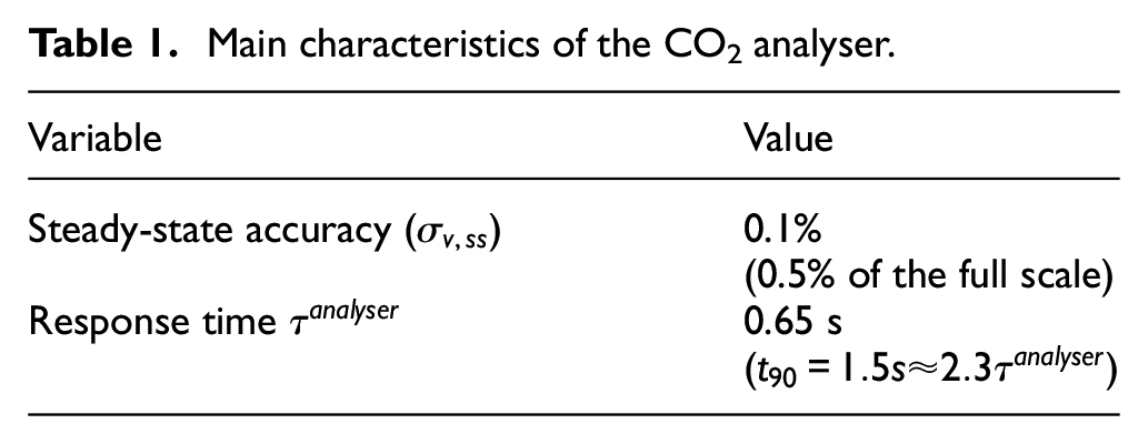
Regarding the tests, three different driving cycles were considered in this work: the NEDC, the worldwide harmonised light-duty cycle (WLTC) and a synthetic driving cycle representing urban conditions. In this sense, the tests cover a wide spectrum of operating conditions and driving dynamics.
Problem description
Figure 1 shows the main issue of exhaust CO2 analysers. In particular, it shows different measured signals in the first acceleration of the NEDC as an example. The upper plot shows the vehicle speed evolution, where the driver tries to follow a predefined driving profile that in this part of the cycle consists on an acceleration from 0 to 15 km/h and back again to 0. Due to the engine start and stop system, the engine starts 3 s after the beginning of the test. At this point, a sudden increase in the fuel mass flow estimation from the ECU and measured air mass flow can be observed in the second and third plots. If the focus is put on the CO2 concentration measured by the test bench analyser (see the fourth plot), the main issue of exhaust gas analysers becomes apparent. The exhaust gas analysers have long response times in comparison with the other engine transducers, meaning that the measured emission concentrations are delayed and filtered with respect to the other engine parameters. In particular, in Figure 1, a smooth increase in the CO2 concentration after the engine start can be observed. It should be noted that this signal has been phased using a constant time offset with the fuel injection provided in the second plot, since the exhaust gas analyser exhibits not only a limited dynamic response but a significant delay because of the exhaust and sampling line transport delay. One can clearly identify an excessive filtered response in the measured CO2 concentration since a sudden increase in the CO2 production after the engine start is expected. In the same way, the fast increase in the CO2 that is expected when the vehicle accelerates as a consequence of the fuelling rate increase does not appear in the measurements. Finally, despite the CO2 measurements, a sudden reduction in the exhaust CO2 concentration to 0% would be expected when the engine is turned off after the vehicle stop.
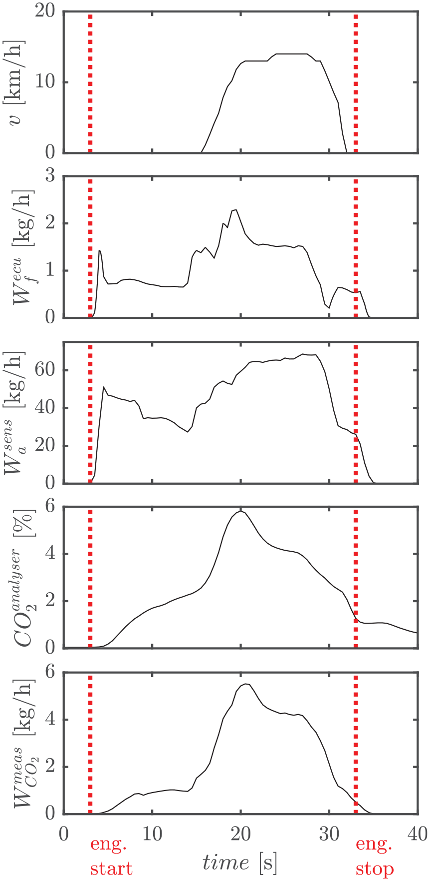
From top to bottom: evolution of velocity, fuel injection estimation by the ECU, air mass flow measured by the engine sensyflow, exhaust CO2 concentration measured with the exhaust gas analyser and computed CO2 mass flow emissions from previous signals.
CO2 emissions (
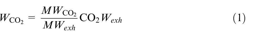
where
A relation between the fuel consumption
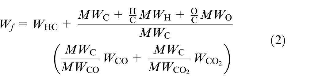
where MW represents the molecular weight of the different species involved (denoted as subscripts
Ratio between CO2 mass flow (
According to the previous paragraph, equation (3) may be simplified with little loss of accuracy to

where
Figure 3 shows an example where the calculated CO2 concentration from the ECU fuel consumption exhibits a very similar pattern to that provided by the exhaust gas analyser. In fact, the CO2 emissions from the ECU estimation of fuel consumption are used in this work to put the analyser raw measurement in phase with the rest of test bench signals by cross-correlation maximisation. 21 In addition, Figure 3 shows discrepancies between raw analyser measurements and the application of equation (3) at both steady and transient conditions. In the case of steady-state operation (e.g. 20 s), some differences appear due to the inaccuracy of ECU fuel estimation and simplifications done in equation (3). Concerning transient conditions (e.g. 5–12 s), the method based on the ECU estimation is not affected by the filtering associated with sensors. This is most notable during periods of fuel cut-off (e.g. 24 s) where the analyser provides non-zero value of CO2 despite the lack of fuel burning.
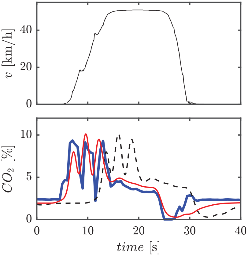
Example of the CO2 signal phasing. Blue: CO2 estimation from ECU signals. Dashed black: raw CO2 measurement from the exhaust gas analyser. Red:
Taking into account the strong and weak points of previous methods to compute the CO2 emissions, the problem addressed in this article is to merge CO2 signals from the analyser and equation (3) to provide the best possible estimation of CO2 in a dynamic cycle.
Proposed approach
KF basics
The problem described in the previous section can be solved using data fusion, where among a wide set of techniques, 22 the KF 23 is one of the most widely used algorithms. A complete description of the algorithm is outside of the scope of the present paper and only the main equations are recalled for the sake of readability. Consider the generic discrete time invariant system
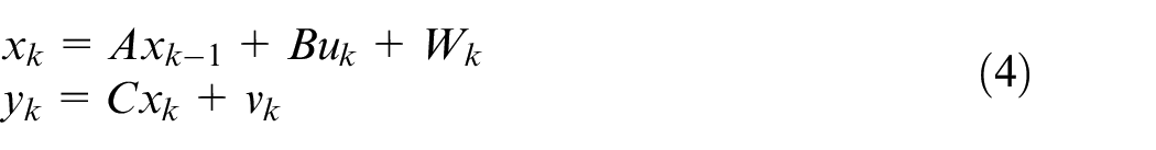
where
The KF
23
provides the optimal solution for the estimation problem of the previously described system (i.e. estimating the state of the system
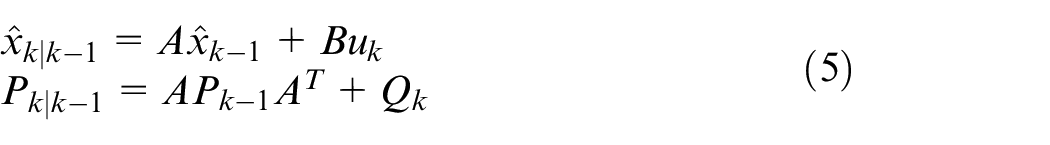
1. Prediction. The model of the system is used to calculate a priori estimations of the state (
2. Update. The previous a priori estimations are improved by applying the Kalman gain (
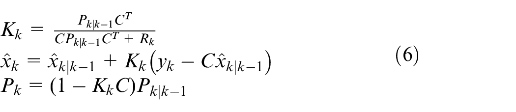
where
The problem addressed in the present work can be identified as a particular case of the general problem described by equations (4)–(6), where
The state (
The input (
The measurement (
Despite the simplicity in the formulation and the performance in practical application of the KF, it is rather complex to find a system that strictly fulfils its requirements, not only because most of the real systems are not linear but also because noises rarely follow a Gaussian distribution and their covariances are not usually a priori known. 22 In addition, the variances of process noise (Q) and measurement noise (R) have a key impact on the performance of the KF. 24
KF with augmented model for drift correction
Taking into account that the ECU-based estimation contains the high-frequency information of the actual CO2 emissions but has some drift, the analyser signal (slow but accurate in steady state) can be used to compensate this drift as proposed in Blanco-Rodriguez
16
for the NOx emissions and

where the state vector
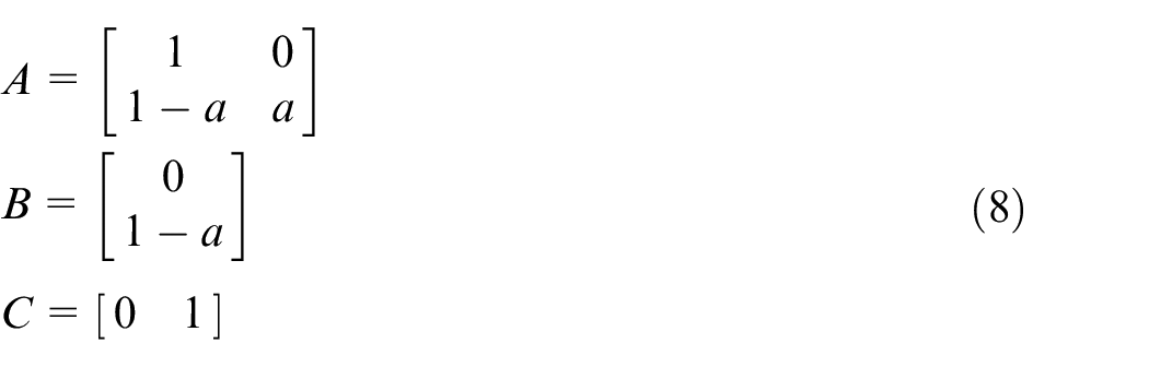
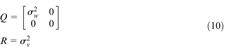
where a is the discrete time version of the system time constant that can be obtained from the analyser response time (see Table 1) and the sample time to convert model from continuous to discrete time. The process noise (

and the output noise (
Note that from the structure of matrix A, it can be observed that
The model implicitly involves a slow evolution in the drift since
The process noise is applied exclusively to the model bias

In addition, provided that the system is linear time invariant (LTI), if the covariances are considered constant, the Kalman gain (K) rapidly tends to a constant value. This value depends on the time response of the analyser (a) and the ratio between process and output covariances (
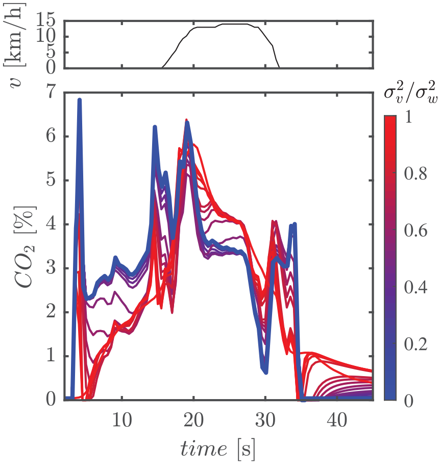
Vehicle speed (top) and CO2 signals. Blue: CO2 estimation from ECU signals. Red: CO2 signal from the exhaust gas analyser. Colorscale: CO2 estimation with the proposed augmented model depending on the
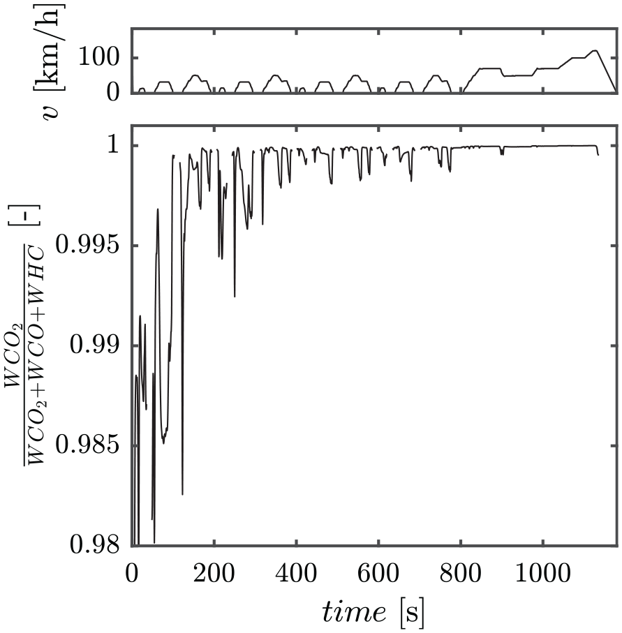
Figure 5 shows the ratio between CO2 emissions obtained from the extended model KF approach and the analyser in three different driving cycles. One can observe how as the
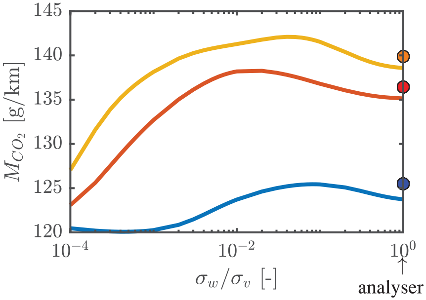
Ratio between CO2 emissions estimation and CO2 from the analyser depending on the
As discussed above, the selection of the proper
Proposed noise tuning method
In particular, the output variance is usually obtained from the analyser accuracy data, generally represented using a standard deviation. In the case of the CO2 analyser, the data sheet of the equipment provides an uncertainty value for steady-state measurement (

where
The general assumption that exhaust gas sensors follow a first-order response 16 leads in the case at hand to
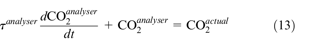
where
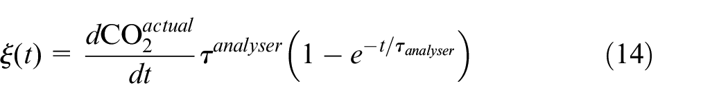
Figure 6 shows an example of the response of the sensor described by equation (13) for two different ramp rates (1% s−1 and 0.5% s−1). In both cases with
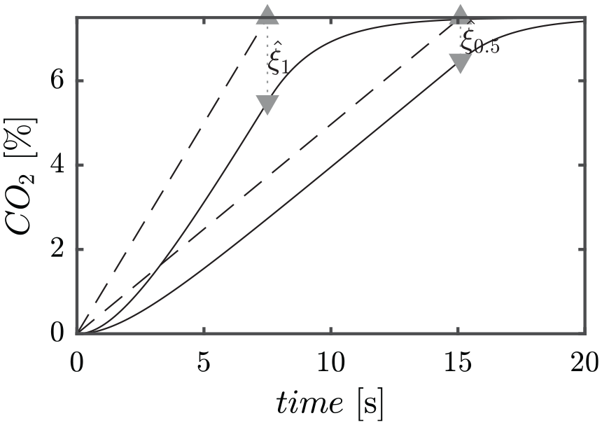
Example theoretical sensor response (continuous lines) considering
It can be observed that according to equation (14), the error increases up to a maximum (
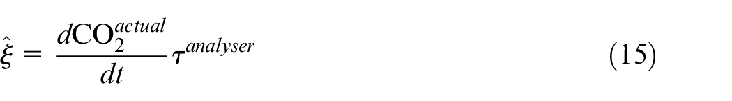
In Figure 7, equation (15) is represented showing the analyser error (
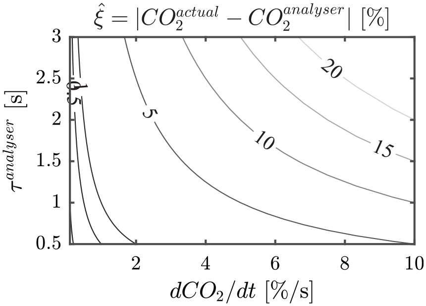
Considered sensor error due to dynamics (
The proposed method consists of assuming

Note that
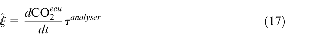
Regarding the estimation of
With respect to the process variance (
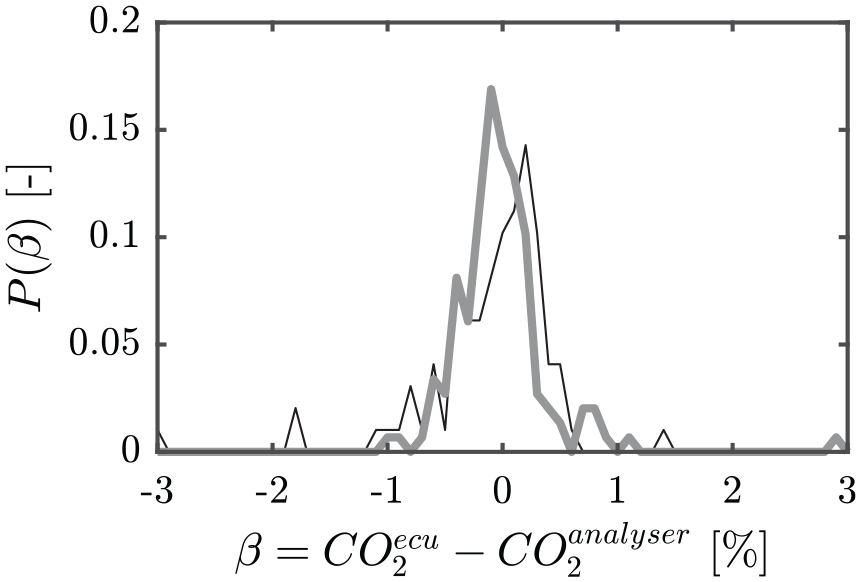
Histogram of the
Results
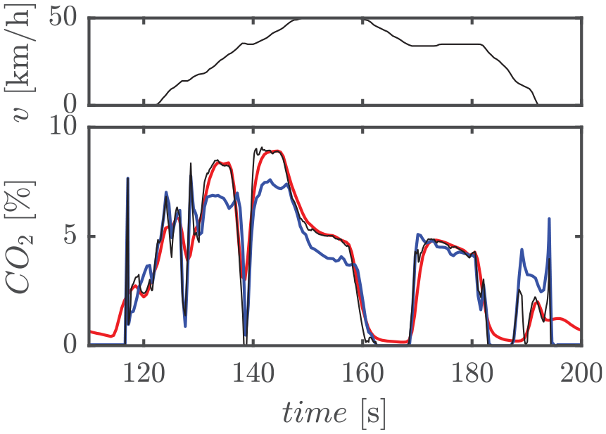
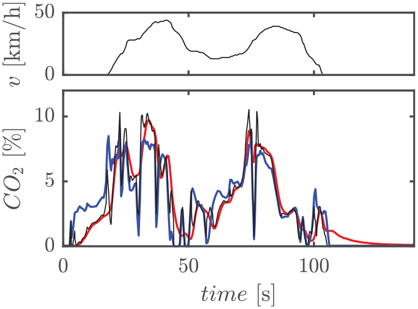
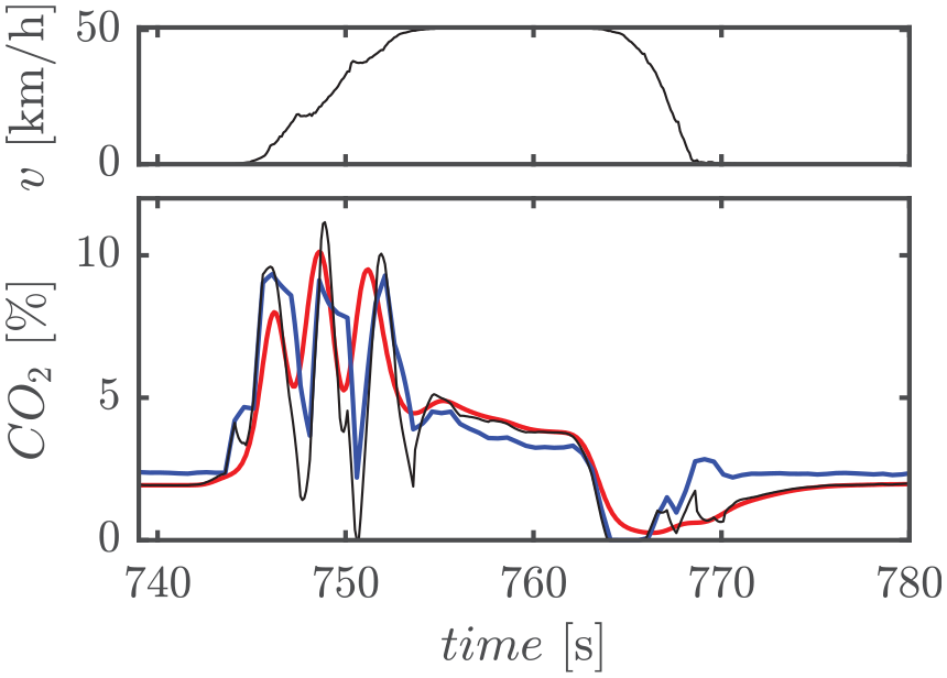
Figures 9–11 show the results obtained at particular segments of three different driving cycles. In the upper plot, the vehicle speed profile can be observed. The three cases show accelerations in the urban range, up to 50 km/h at different rates. In the bottom plot, the evolution of the CO2 concentration can be tracked. It can be clearly observed how, independent of the test, the CO2 estimation provided by the proposed method (black line) tends to the analyser measurement (dashed line) as the rate of change in the CO2 signal is reduced and replicates it in steady-state phases. On the contrary, the CO2 estimation provided by the proposed method tends to the estimation based on the ECU signals (grey line) during dynamic phases. It can be also noted that during step decelerations where there is not fuel injection, unlike the analyser, the proposed estimation leads to null CO2 concentration.
Vehicle speed (top) and CO2 signals (bottom) during a part of the NEDC driving cycle. Blue: CO2 estimation from ECU signals. Red: CO2 signal from the exhaust gas analyser. Black: CO2 estimation with the proposed methodology.
Vehicle speed (top) and CO2 signals (bottom) during a part of the WLTC driving cycle. Blue: CO2 estimation from ECU signals. Red: CO2 signal from the exhaust gas analyser. Black: CO2 estimation with the proposed methodology.
Vehicle speed (top) and CO2 signals (bottom) during a part of an arbitrary urban driving cycle. Blue: CO2 estimation from ECU signals. Red: CO2 signal from the exhaust gas analyser. Black: CO2 estimation with the proposed methodology.
In Figure 12, the differences between the accumulated CO2 emissions obtained from the proposed method and the raw analyser signal are tracked during the three tested cycles. Independent of the driving cycle, in the phases with constant velocity, there are no differences between the values provided by both methods(the line showing the difference between accumulated emissions remains constant), while in the zones with sharp changes in velocity, differences appear to correct the lack of dynamic response of the analyser.
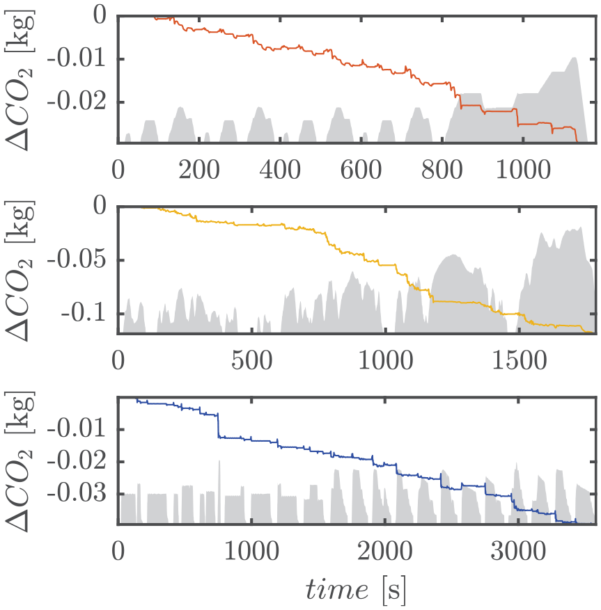
Difference between accumulated CO2 emissions estimated with the proposed method and with the analyser in three driving cycles: NEDC (top), WLTC (medium), and synthetic driving cycle representing urban conditions (bottom). The grey shades represent the velocity profile.
In this way, the proposed approach is able to maintain the steady-state accuracy of the CO2 analyser while keeping the dynamic response of the ECU estimation. To underline this idea, Figure 13 shows the CO2 signals from the three assessed methods during the WLTC in the frequency domain. One may observe how at low frequencies (below 0.2 Hz), the analyser and the proposed method behave similarly, while the ECU estimation slightly underpredicts the CO2 emissions. For higher frequencies (above 0.2 Hz), the dynamic response of the analyser is not high enough to capture the CO2 variations, while the proposed method is able to keep the dynamic response of the ECU estimation.
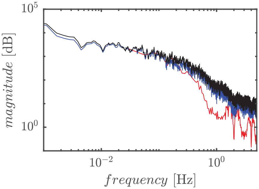
CO2 measurements in the frequency domain for the WLTC. Blue: CO2 estimation from ECU signals. Red: CO2 signal from the exhaust gas analyser. Black: CO2 estimation with the proposed methodology.
In summary, Figure 14 shows the overall CO2 from the three methods, normalised with the analyser results. Discrepancies between the ECU estimation and analyser results range from 4% in the test with lower dynamics (urban) to 14% in the more dynamic WLTC. In particular, the ECU estimation underpredicts the CO2 emissions, as it was also shown in the frequency analysis of Figure 13.
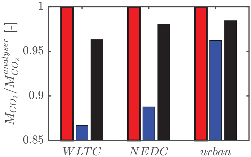
Percentage of CO2 emissions respect to the gas analyser method. Blue: CO2 estimation from ECU signals. Red: CO2 signal from the exhaust gas analyser. Black: CO2 estimation with the proposed methodology.
Regarding the proposed method, differences with the analyser method are below 2% for tests where steady-state phases prevail (like the NEDC or the synthetic urban driving cycle used in this work), but differences up to 4% may appear in driving cycles where dynamics play an important role and then showing that the lack of dynamic response of the analyser has a noticeable impact on the CO2 figures.
Conclusion
This article has discussed the impact of the dynamic limitations of standard CO2 analysers used for engine and vehicle testing over highly transient driving cycles. In those situations, typical analyser response times and transport delays in the sample lines (5–10 s) may lead to noticeable measurement errors. The assessment of the CO2 analyser and ECU-based methods response time and accuracy allows to pose an estimation problem that can be solved by a KF. In particular, the proposed approach is based on the following:
A model augmentation to consider, inside the Kalman filter, the model bias and the sensor dynamics.
Time-dependent covariance
Including the model bias and analyser dynamics in the KF framework allows a compact formulation that can cope with the system dynamics, while the values of
Footnotes
Appendix 1
Declaration of conflicting interests
The author(s) declared no potential conflicts of interest with respect to the research, authorship, and/or publication of this article.
Funding
The author(s) disclosed receipt of the following financial support for the research, authorship, and/or publication of this article: The authors acknowledge the support of Spanish Ministerio de Economia, Industria y Competitividad through project TRA2016-78717-R and Programme GV-BEST ref. BEST/2018/002 for supporting the research stage of B. Pla in the University of Bath.