Sage Journals: Discover world-class research

Abstract

Biaxial tensile tests are of great significance for the characterization of materials. For ductile materials, they allow the representation of the yield strength curve separating elastic and plastic material behavior. Contrary demands regarding the specimen design arise, if a biaxial stress state with the equivalent stress equal or close to the yield strength shall be obtained. On one hand, the specimen shall be of constant thickness and stiffness, in order to allow an unconstrained deformation without undesired lateral strains. On the other hand, stress concentrations arising from the load introduction make a thickened border region necessary, in order to avoid a premature failure of the specimen. The present paper addresses this problem by a multi-objective structural optimization using Evolutionary Algorithms. Well-defined parametric models of biaxial tensile test specimens allow to systematically investigate the influence of the thickness distribution and the sizing of the border region. Additionally, the influence of actuators of constant force compared to actuators of constant displacement are quantified. In all cases, the minimization of the stress difference as well as the actuation effort are considered as objectives. The results allow a deep insight to the optimal definition of biaxial tensile test specimens and are summed up in well-defined design proposals.

Keywords

Biaxial tensile test structural optimization design proposals test specimen topography optimization

Introduction

For the characterization of ductile materials, biaxial tensile tests are of great importance. A single test specimen allows the representation of all relevant biaxial stress states forming the border of elastic deformation. Because of that, biaxial tensile tests are commonly used for characterizing sheets of ductile materials.¹

Cruciform shaped specimens have become important test geometries for biaxial tensile tests.^1,2 Nevertheless, the detailed design of suitable cruciform test specimens poses a challenging engineering question. Targets are an undisturbed uniform stress state in the measuring region and suitable interfaces for loading the specimen. In general, these targets are opposing, as thickened loading interfaces disturb the uniform stress state. In order to find the best layout of biaxial tensile test specimens, numerical optimizations have been widely applied. In the following, a brief review of relevant scientific works is given. For more comprehensive reviews, the reader is referred to Refs.^1,3,4

Demmerle and Boehler⁵ have coupled a Finite Element model with a gradient-free optimization method in order to optimize the geometry of a cruciform tensile test specimen with the target of allowing a homogeneous stress and strain field. A miniaturized cruciform specimen geometry has been optimized by Zhu et al.⁶ Nasdala and Husni⁷ have used numerical optimization to modify the ISO 16842 test specimen with the aim of measuring yield surfaces. Zhao et al.⁸ applied Genetic Algorithms to the optimization problem of sandwich cruciform specimens. A gradient-based optimization algorithm has been used by Makris et al.,⁹ in order to optimize the shape of a specimen for biaxial tensile tests of composites. Genetic Algorithms have been used by Bauer et al.,¹⁰ in order to optimize the shape of test specimens for sheet molding compounds. Recently, Yang et al.¹¹ used Genetic Algorithms for a two-objective optimization of a cruciform test specimen with the aim of maximizing the stress level and minimizing the stress inhomogeneity in the specimen center. Manual optimizations of cruciform specimens for aluminum alloys and steel using Finite Element analyses have been presented by Andrusca et al.^12,13 and Xiao et al.¹⁴ Shao et al.¹⁵ conducted experimental and simulative analyses in order to optimize the geometry of cruciform specimens for evaluation of aluminum alloys under hot stamping conditions. Apart from cruciform specimens, optimization of other biaxial test specimen shapes, like the X0-specimen,^16,17 have been performed.

Besides optimization, sensitivity studies on geometrical parameters of cruciform test specimens have been done using Finite Element analyses.¹⁸ A number of different specimen geometries for performing biaxial testing of multiple alloys under elevated temperature conditions have been experimentally investigated by Abu-Farha et al.² Basic experimental and simulative studies on ideal geometries for polymeric material specimens of biaxial tensile tests have been presented by Hartmann et al.¹⁹ Several cruciform specimen designs for testing sheet molding compounds have been investigated experimentally and numerically by Lang et al.²⁰ and Schemmann et al.²¹ Geometry designs for increasing the measurable plastic strain rates have been presented by Hou et al.²²

This brief literature survey underlines the continuing research interest in optimizing the shape and topology of cruciform biaxial tensile specimens.

The present publication enriches the knowledge of optimal designs of cruciform test specimens for biaxial tension by giving fundamental design proposals based on comprehensive structural optimization. After outlining the basic targets and restrictions for biaxial tensile specimens, a general parametric Finite Element model is presented, allowing fundamental analyses of cruciform tensile test specimens. Integrating the parametric Finite Element model into a holistic optimization framework, aiming for homogeneous stress distributions and minimal actuation effort, then allows the well-founded deduction of design proposals by quantitative evaluations.

Problem definition and basic assumptions

Aims and limitations

For the present investigation, a suitable framework is presented that allows to optimize the design of a biaxial tensile test specimen, schematically shown in Figure 1, in order to best match the target stress state over the measuring region by a low actuation effort. Therefore, two objectives are taken into account:

Minimization of the difference between the present and target stress state over the measuring region of the specimen.

Minimization of the actuation effort needed for obtaining the desired stress state.

Figure 1.

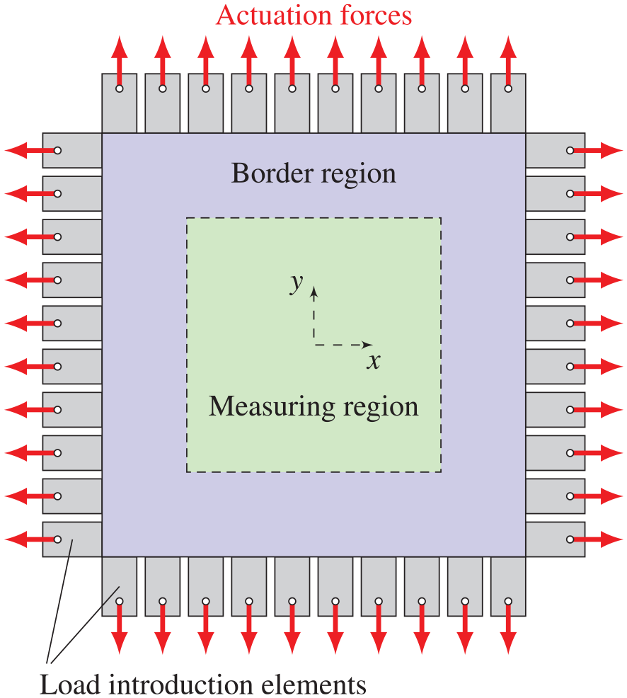
General layout of the test specimen with measuring region, border region and load introduction elements.

For practical reasons, the measuring region is surrounded by a border region. At the edges of the border region, discrete actuators are placed for loading the specimen. To make sure that the border region and actuators do not fail before reaching the target stress state in the measuring region, two structural constraints are taken into account:

No premature failure of the measuring region is allowed.

The actuators must withstand at least twice the load required for obtaining the target stress state.

In order to reach the defined objectives under the given practical constraints, a number of questions concerning the optimal specimen design arise:

What is the optimal size of the border region surrounding the measuring region?

Which thickness topography of the border region is optimal?

What is the optimal thickness of the load introduction?

Which number of discrete actuators are needed for best results?

Are actuators of constant force or constant displacement preferable?

The presented optimization framework has been applied to answer these questions and to quantitatively compare different design proposals regarding their benefits.

In order to allow the deduction of general conclusions, the structural problem is simplified to a single load case. This allows the understanding and evaluation of the obtained results without overconstraining the applicability.

Target stress state

The purpose of the biaxial tensile test is to reproduce the yield strength curve in the first quadrant for plane stress states. Considering isotropic materials with ductile behavior, this curve can be idealized by the von Mises criterion

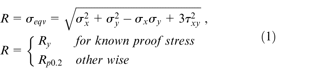
\begin{matrix} R = σ_{eqv} = \sqrt{σ_{x}^{2} + σ_{y}^{2} - σ_{x} σ_{y} + 3 τ_{xy}^{2}}, \\ R = {\begin{matrix} R_{y} & for known proof stress \\ R_{p 0.2} & other wise \end{matrix} \end{matrix}

(1)

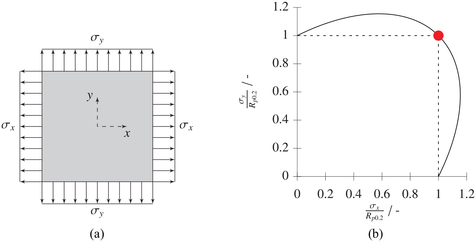
with the material strength $R$ being either the yield strength $R_{y}$ or the 0.2% proof stress $R_{p 0.2}$ , $σ_{eqv}$ the von Mises equivalent stress, $σ_{x}$ the normal stress in $x$ -direction, $σ_{y}$ the normal stress in $y$ -direction and $τ_{xy}$ the shear stress in the $x$ - $y$ -plane. Assuming a principal stress condition ( $τ_{xy} = 0$ ), the stress state shown in Figure 2(a) results.

Figure 2.

Plane principal stress state (a) and corresponding von Mises yield strength curve for isotropic materials with 0.2% proof stress $R_{p 0.2}$ and marked state of interest $σ_{x} = σ_{y} = R_{p 0.2}$ (b).

In the following, the 0.2% proof stress $R_{p 0.2}$ is assumed as the material strength $R$ according to equation (1). Figure 2(b) depicts the corresponding yield strength curve, normalized by $R_{p 0.2}$ . Highlighted in Figure 2(b) is the point $σ_{x} = σ_{y} = R_{p 0.2}$ that is considered in the following as the target stress state for the biaxial tensile test. It shall be noticed that simplifying the biaxial tensile test to a single point $σ_{x} = σ_{y}$ does not allow to reproduce the whole stress curve illustrated in Figure 2(b). This limitation does not allow a direct transfer of the resulting designs for reproducing other stress states. Nevertheless, it still allows the deduction of exemplary design proposals in accordance with the aims of the present paper.

General outline of the test specimen geometry

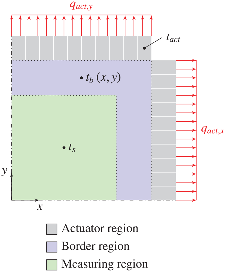
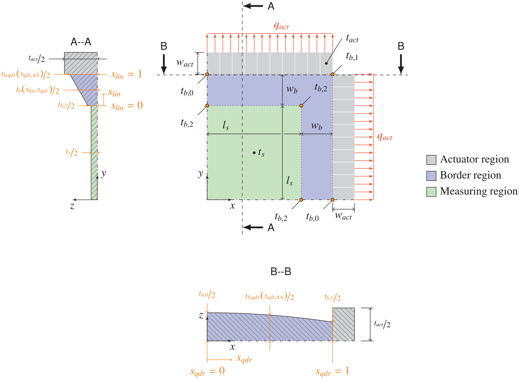
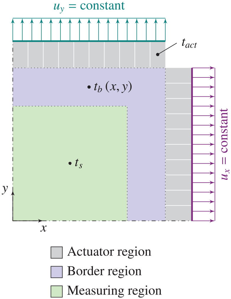
Figure 3 shows the assumed general layout of the test specimen. The specimen has an integral design with basically three regions. In the measuring region, the target stress state shall be obtained as well as possible. The border region transfers the actuator forces to the measuring region and shall allow the decay of stress concentrations arising from the load introduction. Finally, the actuator region models actuators of finite stiffness. It can be split into multiple regions for modeling discrete actuators, as illustrated. At the outer borders, the actuator loads are introduced, modeling generic actuators.

Figure 3.

General layout of the test specimen.

Planes of symmetry

Per definition, the problem of the biaxial tensile test is symmetric to the $x$ - $y$ -, $x$ - $z$ -, and $y$ - $z$ -plane, as shown in Figure 2(a). For the special case of $σ_{x} = σ_{y}$ , a third and fourth plane of symmetry can be found by a rotating the $x$ - $z$ -plane $\pm 45 °$ around the $z$ -axis. The latter two planes of symmetry are not considered here, in order not to restrain the universality of the models.

Load introduction

As outlined in Figure 2(a), loads are introduced orthogonal to the specimen edges as tension loads. Ideally, the load introduction would be done by actuators of infinite small width along the edge, in order not to constrain the transverse strain of the specimen. For practical applications, actuators shall be modeled with a finite width closely spaced next to each other, in order to approximate the line load as closely as possible. Constructive details of the loading and actuation are not considered in the present investigation. As shown in Figure 3, a force-constant loading of each discrete actuator is assumed, as it can be practically achieved by an individual hydraulic or electric cylinder. Additionally, an actuation of constant displacement of each actuator will be considered in the optimization study. For practical purposes, a constant-displacement loading of each actuator can be achieved by a single hydraulic or electric cylinder at each specimen edge.

Thicknesses

As illustrated in Figure 3, the test specimens can be subdivided into three regions, in order to specify the thickness distributions $t (x, y)$ :

measuring region with given constant specimen thickness $t_{s}$ ,

border region with unknown thickness distribution $t_{b} (x, y)$ ,

actuator region with unknown constant thickness $t_{act}$ .

A main question concerning the optimal layout of the test specimen addresses the thickness distribution $t_{b} (x, y)$ of the border region, as it has to fulfill two conflicting objectives. On one hand, the thickness should ideally be identical to the thickness of the measuring region, in order to avoid stiffness discontinuities at the interface between the measuring region and the border region. On the other hand, the border region must be thicker than the measuring region to allow the decay of stress discontinuities without static failure.

Optimization framework

In the following, the optimization framework developed for the present investigation is outlined. In agreement with the aims of the present paper, emphasis has been put on simplifying the optimization problem as much as possible but still allowing sufficient freedom for the design of the specimen topography.

Parametric model

A parametric model of the test specimen with a variable topography of the border around the measuring region is defined.

The length of the measuring region of the quarter model is given as an input parameter $l_{s}$ , so that a quadratic specimen is assumed. The width of the border region can be varied during the optimization by the variable $w_{b}$ . Additionally, the width of the actuator region is variably defined by $w_{act}$ , as shown in Figure 4.

Figure 4.

Parameterized test specimen with symmetry to the $x$ - $y$ -, $x$ - $z$ -, and $y$ - $z$ -plane.

The thickness of the measuring region is assumed to be constant with a predefined value $t_{s}$ . The actuator region thickness is also constant and defined by the design variable $t_{act}$ .

Emphasis has been put on well-founded definitions of the border region thicknesses $t_{b} (x, y)$ . The main aim is to provide a wide range of valid thickness distributions by a low number of variables. Therefore, the thickness of the border region may vary quadratically parallel to the edges of the measuring region, in order to allow counteracting their bending deformation. As outlined in cut B- -B of Figure 4, the derivative of the quadratic function is assumed to be zero at the symmetry planes. Hence, the quadratic thickness distribution is described by

t_{b, qdr} (s_{qdr}) = t_{b, 0} - s_{qdr}^{2} \cdot (t_{b, 0} - t_{b, 1})

(2)

of the normalized coordinate $s_{qdr} \in [0, 1]$ .

Additionally, the border region thickness can vary linearly between the actuator region and the measuring region, as shown in cut A- -A of Figure 4. Therefore, the thickness distribution is enhanced by a linear variation

t_{b} (s_{lin}, s_{qdr}) = [t_{b, qdr} (s_{qdr}) - t_{b, 2}] \cdot s_{lin} + t_{b, 2}

(3)

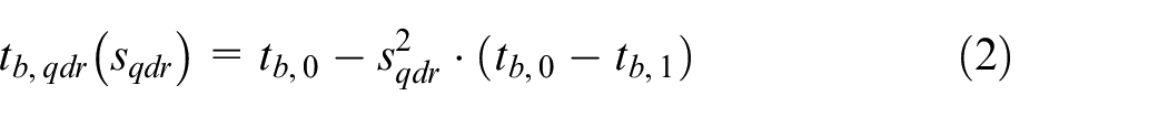
over the normalized coordinate $s_{lin} \in [0, 1]$ . In Figure 4, $t_{b, qdr} (s_{qdr, AA})$ is the thickness at the cut position $s_{qdr, AA}$ , according to equation (2). The linear variation allows the decay of stress concentrations arising from the load introduction by the discrete actuators.

Using the linear and quadratic thickness definitions of equation (3), only three variables $t_{b, 0}$ , $t_{b, 1}$ , and $t_{b, 2}$ are needed to describe the thickness distribution over the border region $t_{b} (x, y)$ .

The actuators are defined by their number $n_{act}$ along each border edge of the quarter model and their line force $q_{act}$ . The line force $q_{act}$ is applied at the outer edges of the actuators which transfer the load to the border of the specimen. By that, the main characteristics of discrete real-world actuators of finite stiffness are modeled.

Optimization problem

Taking the outlined objectives and constraints into account, the resulting multi-objective optimization problem is stated as

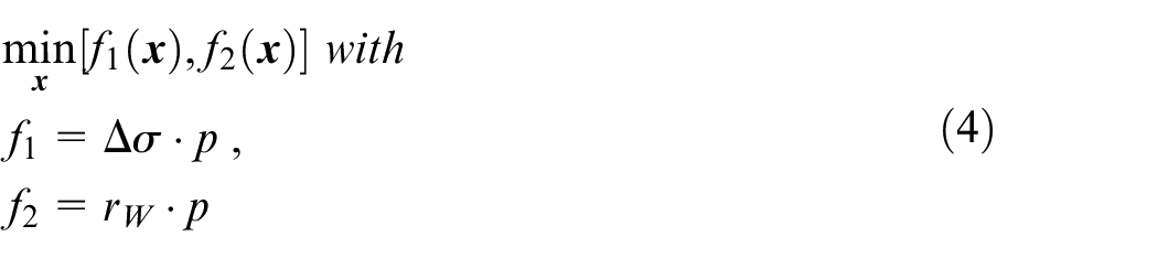
\begin{matrix} min_{x} [f_{1} (x), f_{2} (x)] with \\ f_{1} = Δ σ \cdot p, \\ f_{2} = r_{W} \cdot p \end{matrix}

(4)

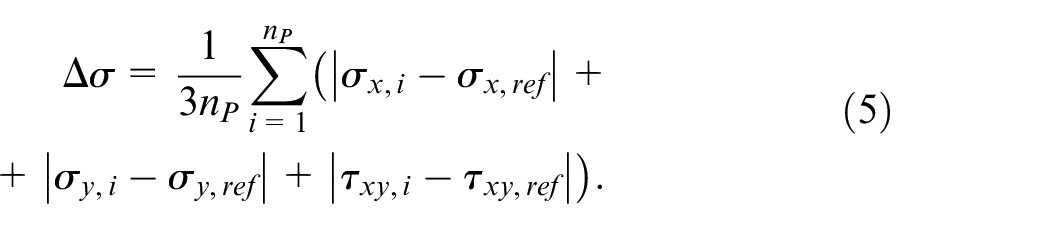
where $x_{\min} \leq x \leq x_{\max}$ contains the design variables, $Δ σ$ denotes the stress difference, $r_{W}$ the actuation effort and $p$ the total penalty factor.

The stress difference is quantified by the mean absolute deviation of the plane stress components $σ_{x, i}$ , $σ_{y, i}$ , $τ_{xy, i}$ at the centers $(x_{i}, y_{i})$ of the $i = 1, \dots, n_{P}$ Finite Elements discretizing the measuring region from the target stress state $σ_{x, ref}$ , $σ_{y, ref}$ , $τ_{xy, ref}$ :

\begin{matrix} Δ σ = \frac{1}{3 n_{P}} \sum_{i = 1}^{n_{P}} (| σ_{x, i} - σ_{x, ref} | + \\ + | σ_{y, i} - σ_{y, ref} | + | τ_{xy, i} - τ_{xy, ref} |) . \end{matrix}

(5)

The actuation effort is quantified by the ratio

r_{W} = \frac{W_{total}}{W_{res}}

(6)

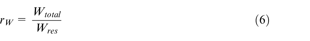
of the total strain energy $W_{total}$ in the measuring region and the border region over the strain energy $W_{res}$ in the measuring region. Hence, the minimal actuation effort is defined by $r_{W} = 1$ , where the complete strain energy is used for the deformation of the measuring region. For example, this would be achieved by eliminating the border region ( $w_{b} = 0$ ).

Besides the two objectives, optimization constraints penalize infeasible and invalid designs. If an optimization constraint is violated, the objective values are multiplied with the penalization parameter $p$ , several orders of magnitudes larger than the objectives.

Infeasible designs include specimens with a total actuator force

F_{total} = 2 q_{act} \cdot (l_{s} + w_{b})

(7)

lower than the minimum force

F_{\min} = (σ_{x, ref} + σ_{y, ref} + 2 τ_{xy, ref}) \cdot l_{s} \cdot t_{s}

(8)

required for obtaining the target stress state in the measuring region.

Invalid designs are obtained if the ratio of the 0.2% proof stress of the material to the maximum equivalent stress in the border region ( $σ_{eqv, \max, b}$ ) or in the actuator region ( $σ_{eqv, \max, act}$ ) is below one or two, respectively. This constraint ensures that the border and actuator region of the specimen do not fail before the target stress state in the measuring region is reached.

The penalty factors for infeasible and invalid designs are therefore given by

p_{1} = {\begin{matrix} \frac{F_{\min}}{F_{total}} \cdot 10^{5} & if F_{total} < F_{\min} \\ 1 & other wise, \end{matrix}

(9)

p_{2} = {\begin{matrix} \frac{σ_{eqv, \max, b}}{R_{p 0.2}} \cdot 10^{5} & if \frac{R_{p 0.2}}{σ_{eqv, \max, b}} < 1 \\ 1 & other wise, \end{matrix}

(10)

p_{3} = {\begin{matrix} \frac{2 σ_{eqv, \max, act}}{R_{p 0.2}} \cdot 10^{5} & if \frac{R_{p 0.2}}{σ_{eqv, \max, act}} < 2 \\ 1 & other wise \end{matrix}

(11)

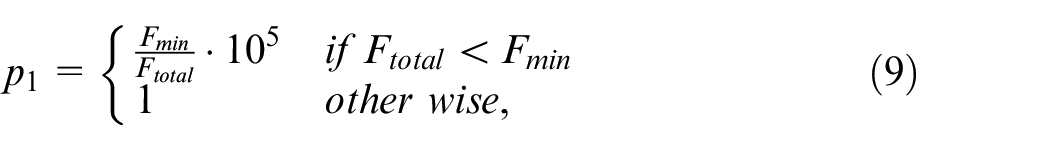
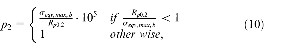
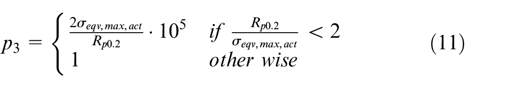
and multiplied to the total penalty factor used in equation (4):

p = p_{1} \cdot p_{2} \cdot p_{3} .

(12)

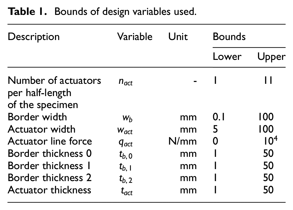
For the present optimization problem, the bounds $x_{\min}$ and $x_{\max}$ of the design variables are given in Table 1. The constant model parameters considered here are listed in Table 2, assuming aluminum Al2024 as the material of the whole structure. It shall be noted that the specific sizing is chosen generically. Due to the linearity of the problem, sizes and forces can be scaled for practical realization.

Table 1.

Bounds of design variables used.

Description	Variable	Unit	Bounds
Description	Variable	Unit	Lower	Upper
Number of actuators per half-length of the specimen	$n_{act}$	-	1	11
Border width	$w_{b}$	mm	0.1	100
Actuator width	$w_{act}$	mm	5	100
Actuator line force	$q_{act}$	N/mm	0	$10^{4}$
Border thickness 0	$t_{b, 0}$	mm	1	50
Border thickness 1	$t_{b, 1}$	mm	1	50
Border thickness 2	$t_{b, 2}$	mm	1	50
Actuator thickness	$t_{act}$	mm	1	50

Table 2.

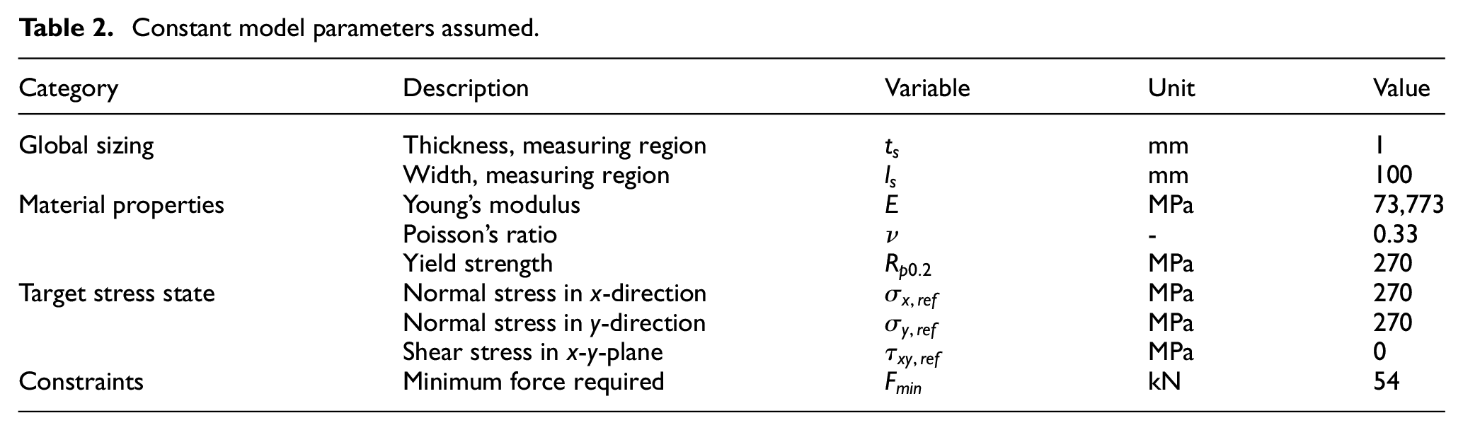
Constant model parameters assumed.

Category	Description	Variable	Unit	Value
Global sizing	Thickness, measuring region	$t_{s}$	mm	1
	Width, measuring region	$l_{s}$	mm	100
Material properties	Young’s modulus	$E$	MPa	73,773
	Poisson’s ratio	$ν$	-	0.33
	Yield strength	$R_{p 0.2}$	MPa	270
Target stress state	Normal stress in $x$ -direction	$σ_{x, ref}$	MPa	270
	Normal stress in $y$ -direction	$σ_{y, ref}$	MPa	270
	Shear stress in $x$ - $y$ -plane	$τ_{xy, ref}$	MPa	0
Constraints	Minimum force required	$F_{\min}$	kN	54

Evolutionary optimization

Equation (4) defines a multi-objective optimization problem consisting of discrete and continuous design variables. For solving this kind of optimization problems, Evolutionary Algorithms are well suited. The outline of the optimization framework applied is shown in Figure 5.

Figure 5.

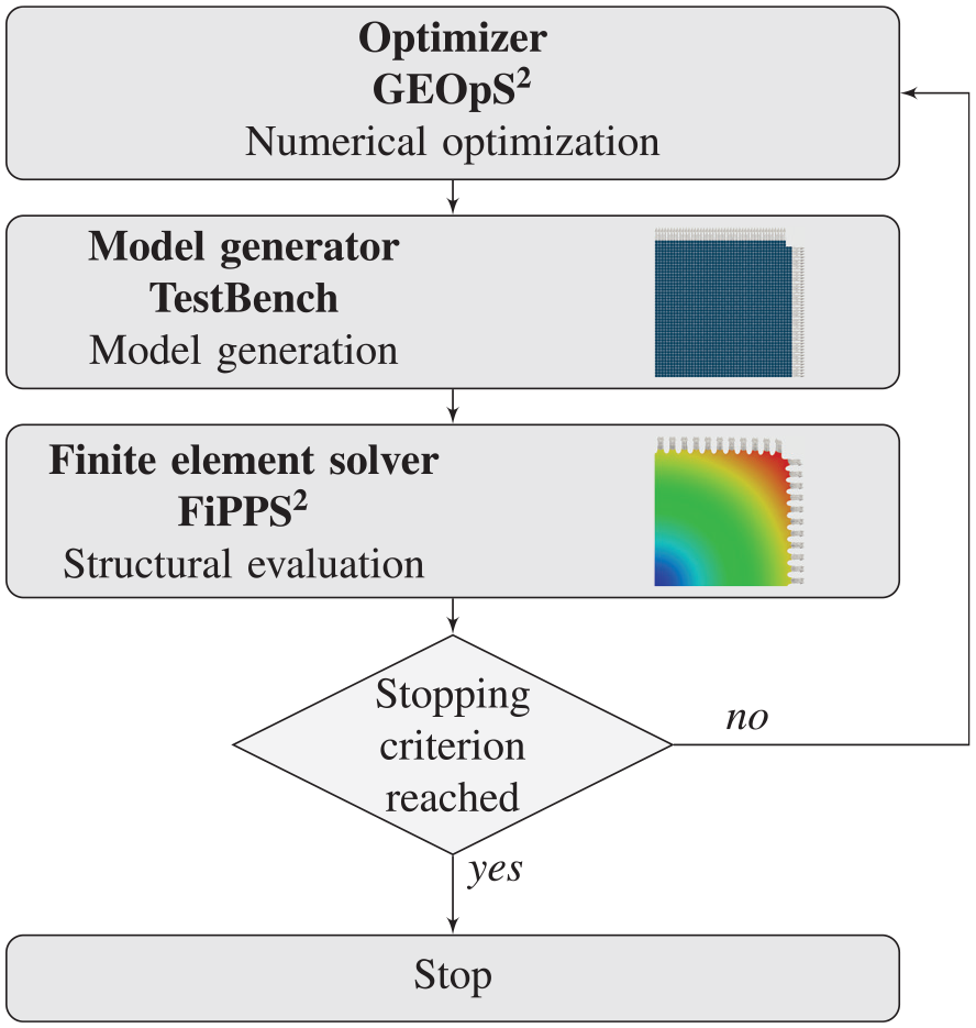
Outline of the optimization framework.

Basis of the optimization framework is the in-house optimization tool GEOpS2, developed by Kaletta.²³ GEOpS2 is based on Evolutionary Algorithms and has been successfully applied to various aerostructural optimization tasks.^24–27 High efficiency is gained by massive parallelization of the evaluation of designs.

GEOpS2 uses Genetic Algorithms (GA), Evolution Strategies (ES) and Differential Evolution (DE) as optimization algorithms.

Structural evaluation and Finite Element model

The customized model generator TestBench sets up the Finite Element model for structural evaluation. The two-dimensional structure is discretized by quadratic quadrilateral 8-node shell elements with the mesh density shown in Figure 6.

Figure 6.

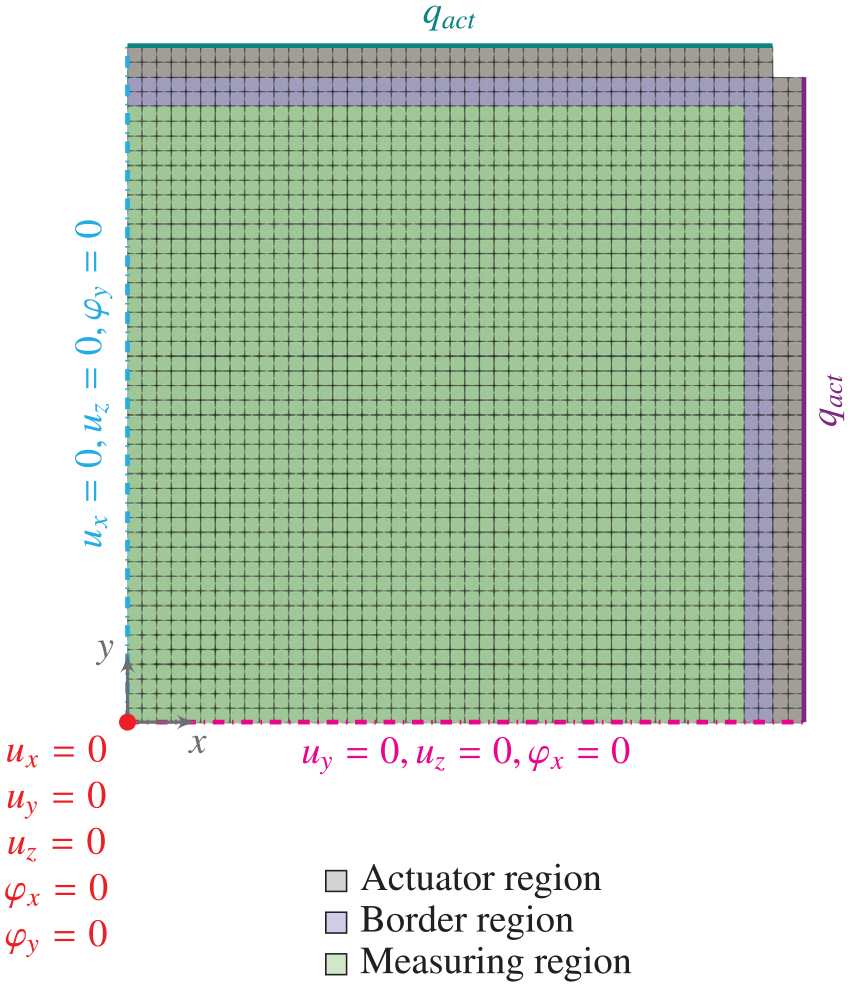
Finite Element mesh of test specimen with displacement boundary conditions and line forces marked.

In order to take the symmetry to the $x$ - $y$ -plane into account, a midsurface model is used. Hence, the reference plane of the shell elements equals the $x$ - $y$ -midsurface of the specimen, as outlined in Figure 4.

The displacement boundary conditions are specified in order to account for the two remaining symmetry planes $x$ - $z$ and $y$ - $z$ . Therefore, all translations as well as the rotations $φ$ around the $x$ - and $y$ -axis are fixed at the node in the origin $(0, 0)$ . Along the left edge ( $x = 0$ ) translations in $x$ - and $z$ -direction $u_{x}$ , $u_{z}$ , as well as the rotations around the $y$ -axis $φ_{y}$ are fixed. Analogous, along the bottom edge ( $y = 0$ ) translations in $y$ - and $z$ -direction $u_{y}$ , $u_{z}$ , as well as the rotations around the $x$ -axis $φ_{x}$ are set to zero.

Loads are applied at the top and right edge as line loads. Therefore, the line loads are transferred to equivalent nodal forces, taking the quadratic shape functions of the shell elements into account.

Distinct element properties are used for the actuator, border and measuring region, allowing to take individual failure criteria into account and to ease the post-processing.

The model is solved by the in-house linear static Finite Element solver FiPPS2.

Results

The following section describes the optimization results by successively increasing the degree of freedom of the parameterized test specimen.

Baseline design

At first, baseline results are obtained by applying the optimization method with the simplification of a constant thickness

t_{b} = t_{b, 0} = t_{b, 1} = t_{b, 2}

(13)

of the border region.

After reaching the stopping criterion of the optimization process, a number of Pareto-optimal solutions is obtained. In terms of multi-objective optimization, a Pareto-optimal solution is a solution not dominated by any other solution. The set of all Pareto-optimal solutions obtained forms the Pareto front which is shown in Figure 7.

Figure 7.

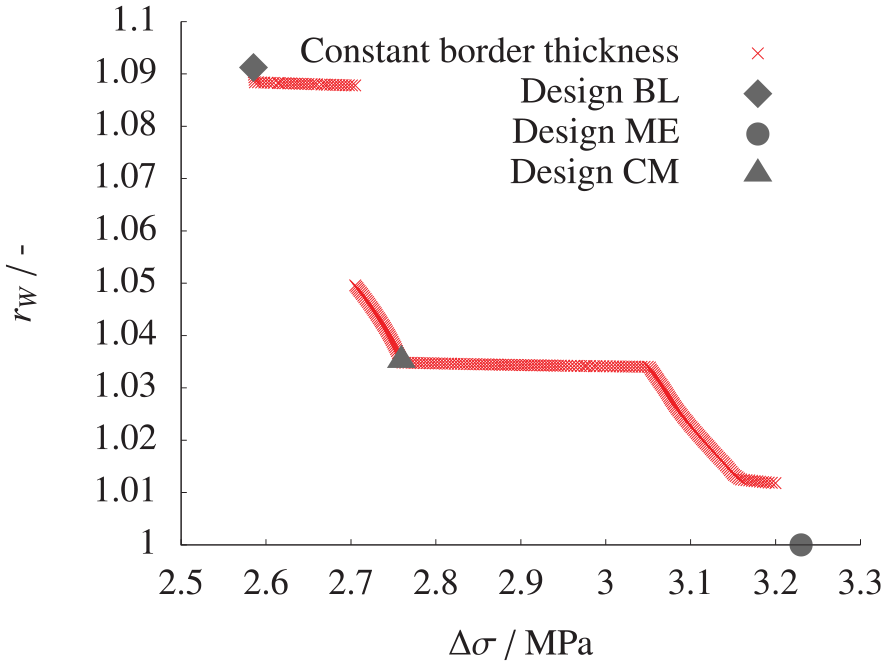
Pareto front of the optimization with constant border thickness with baseline design (BL), design of minimal actuation effort (ME) and compromise design (CM) marked.

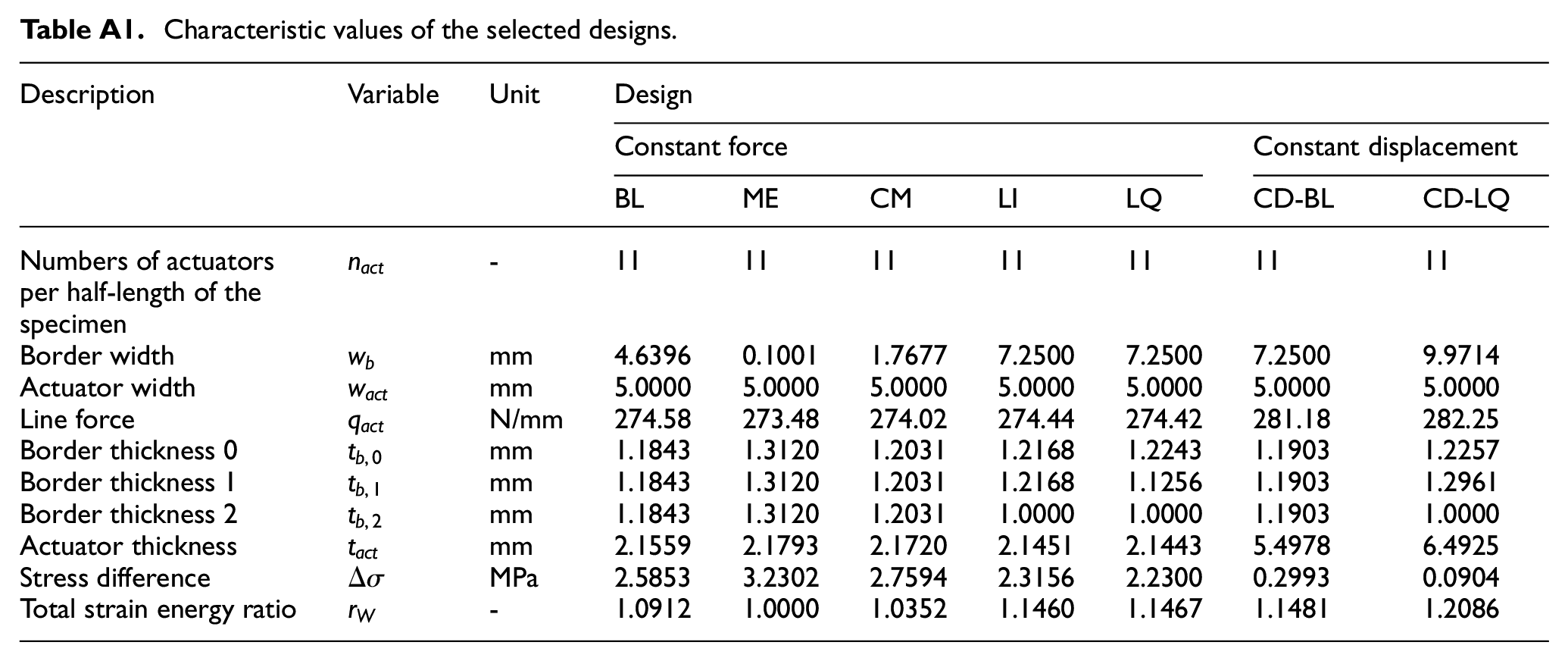
It can be noticed that the stress difference $Δ σ$ and the strain energy ratio $r_{W}$ are conflicting objectives. The arbitrary weighting of the two objectives allows a problem-dependent selection of a specific test specimen geometry out of the solutions provided by the Pareto front. The discontinuous character of the Pareto front is due to the limited size of the Finite Elements discretizing the structural model. By that, only finite sizing steps are possible, leading to gaps in the Pareto front. As they do not effect the validity and interpretability of the results, this deficiency is acceptable for the present investigation.

In order to highlight the main characteristics of the solutions obtained and to derive a baseline design, three distinct designs are discussed in the following. Namely, these are the solution of minimal actuation effort (ME), the solution of minimal stress difference, denoted as the baseline solution (BL), and a compromise solution (CM), as marked in Figure 7. The abbreviations used for characterizing all designs discussed are given in Table 3. For the sake of clarity, the characteristic values as well as the objective function values of all designs discussed are listed in Table A1 in the Appendix.

Table 3.

Nomenclature of designs discussed.

Abbreviation	Description
BL	Baseline design (minimum stress difference using constant border thickness)
ME	Design of minimal actuation effort
CM	Compromise design
LI	Design with minimum stress difference using linear border thickness
LQ	Design with minimum stress difference using linear and quadratic border thickness
CD-BL	Baseline design (minimum stress difference using constant border thickness) obtained with actuators of constant displacement
CD-LQ	Design with minimum stress difference using linear and quadratic border thickness and actuators of constant displacement

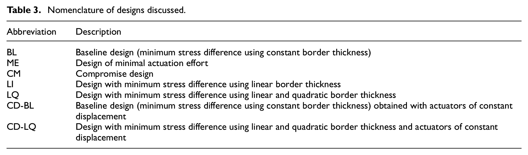
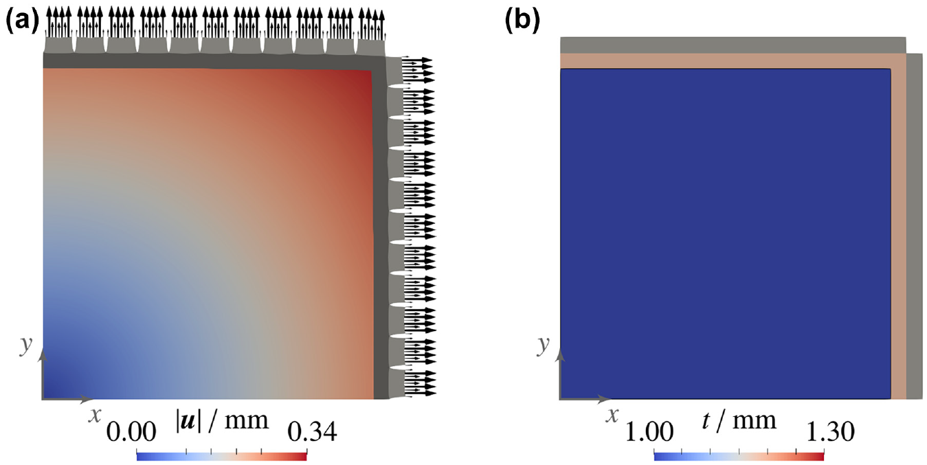
Figure 8 shows the deformation behavior as well as the thickness of the border region and the measuring region. As expected, the number of actuators is set to its maximum value of 11 actuators per half length of the specimen, in order to keep the lateral strains as low as possible. A border region with a width $w_{b} = 4.66 mm$ and a thickness $t_{b} = 1.18 mm$ results, whilst the actuator width is kept to its minimum $w_{act} = 5.00 mm$ . The actuator thickness is increased, compared to the border region, and set to $t_{act} = 2.16 mm$ .

Figure 8.

Design BL – Deformation behavior and structural thickness: (a) displacement vector sum $| u |$ over the measuring region (deformations scaled by factor 50) and (b) structural thickness t over the measuring region and the border region.

As the distribution of the stress components in the measuring region (see Figure 9) shows, the stress concentrations are mainly kept in the border region, in order to avoid deviations from an homogeneous stress state in the measuring region. In order to satisfy the failure criterion defined by equation (10), the border region has to be thicker than the measuring region. This, on the other hand, leads to stress deviations in the measuring region, best visible in the shear stress (see Figure 9(c)) and equivalent stress distribution (see Figure 9(d)), as the deformation of the edges of the measuring region is restricted by the increased stiffness of the border region.

Figure 9.

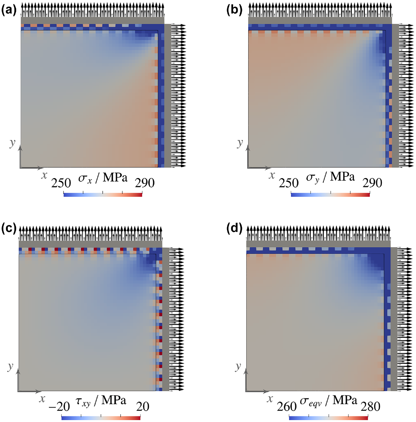
Design BL – Resulting stress distributions: (a) normal stress $σ_{x}$ over the measuring region and the border region, (b) normal stress $σ_{y}$ over the measuring region and the border region, (c) shear stress $τ_{xy}$ over the measuring region and the border region, and (d) equivalent stress $σ_{eqv}$ over the measuring region and the border region.

Therefore, a specimen with constant border thickness only allows compromise solutions. It does not permit to perfectly achieve the biaxial tensile state $σ_{x} = σ_{y} = R_{p 0.2}$ without premature failure of the border region.

As the Pareto front (see Figure 7) shows, varying the sizes of the border region still allows a weighting of the actuation effort and the stress difference. Designs ME and CM, marked in the Pareto front (Figure 7), illustrate this possibility. Design ME has the smallest actuation effort $r_{W} = 1.00$ and is detailed in Figure A1 in the Appendix. The minimized actuation effort is obtained by setting the border width to the lower limit $w_{b} = 0.10 mm$ . By that, the strain energy is almost fully used to deform the measuring region. As the stress concentrations cannot be kept in the border region, they are significantly effecting the stress state in the measuring region, leading to an increased stress difference $Δ σ$ . Design CM (see Figure A2 in the Appendix) represents a compromise solution between a minimized stress difference (BL) and a minimal actuation effort (ME). As visible in Table A1, the border width is decreased by 62%, compared to design BL, whilst the border thickness is slightly increased.

Influence of border thickness definition

The baseline configuration with constant thickness of the border region is compared with thickness definitions of higher degree of freedom:

linear border thickness with the simplification $t_{b, 0} = t_{b, 1}$ ,

linear and quadratic border thickness with separate definition of $t_{b, 0}$ and $t_{b, 1}$ .

In order to maintain the continuity of the thickness distribution between the result and border region, in both cases $t_{b, 2} = t_{s} = 1 mm$ is defined.

Figure 10 shows the resulting Pareto fronts in comparison to the Pareto front obtained with constant thickness of the border region. In each Pareto front, the design with the lowest stress difference is marked for further discussion. It is noticeable, that an increased degree of freedom regarding the thickness definition leads to a better possible matching of the target stress state, as smaller minimal stress differences $Δ σ$ are obtained.

Figure 10.

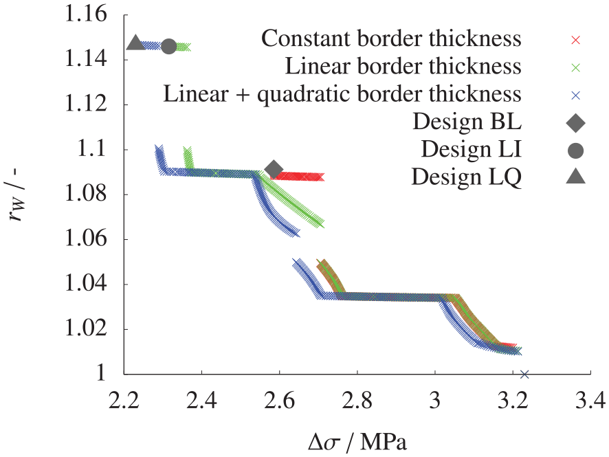
Pareto fronts obtained with different thickness definitions and marked designs of minimal stress difference $Δ σ$ using constant border thickness (BL), linear border thickness (LI) and linear + quadratic border thickness (LQ).

The design LI using the linear thickness definition is shown in Figure A3 in the Appendix. As visible in Figure A3(b), the thickness of the border region increases linearly toward the actuator region. This allows to keep the stress concentrations in the border region without premature failure. By linear reduction of the border thickness toward the measuring region, stiffness discontinuities are avoided. This allows a better matching of target stress state than the baseline design BL, when comparing $Δ σ$ in Table A1. On the other hand, the border region of design LI is enlarged compared to design BL, in order to make use of the linear thickness reduction toward the measuring region. This leads to a slightly increased actuation effort compared to the baseline solution with constant border thickness, as visible in Figure 10 and Table A1. Taking a closer look at the shear stress distribution shown in Figure A3(e), still an undesired shearing in the corner of the measuring region can be observed. This is caused by the increased stiffness of the specimen resulting from the thickened border region.

Reducing the aforementioned bending deformation of the edges of the measuring region was the main motivation for investigating a quadratic variation of the border region thickness over the specimen length and width. The Pareto front in Figure 10 shows that this supplementary design freedom allows a further minimization of the stress difference $Δ σ$ without the need to increase the actuation effort, compared to the solution with linear thickness variation only. The corresponding design LQ is shown in Figure A4 in the Appendix. Again, the linear thickness variation is used to increase the border region thickness toward the actuation region. Additionally, the quadratic thickness variation along the specimen edges is used for reducing the thickness toward the specimen corner. In combination, the obtained thickness distribution again allows to keep the stress concentrations in the border region without its failure. As expected, the quadratic thickness reduction toward the corner allows a reduction of the shearing of the measuring region by reducing the stiffness of the border region close to the specimen corner. By that, the stress state is better met than with designs BL and LI. Nevertheless, an undesired shear stress partly remains (see Figure A4(e)).

Influence of actuators with constant displacement

In order to complete the study, the results obtained with constant-force actuation are compared to results with constant-displacement actuation. Therefore, the optimization runs with

constant border thickness (BL) and

linear and quadratic border thickness variation (LQ)

have been repeated for actuators of constant displacement. This is ensured by coupling the displacements in $x$ -direction $u_{x}$ of the outer edge of the actuator region acting in $x$ -directions and coupling the displacements in $y$ -direction $u_{y}$ of the outer edge of the actuator region acting in $y$ -directions, as depicted in Figure 11. By that, the line force is generally non-uniform along the specimen edge, depending on the stiffness variations over the specimen. In contrast, the force-constant actuation generally results in inhomogeneous displacements over each edge, due to stiffness variations over the specimen. Practically, a constant displacement-constant actuation can be achieved by using a single displacement-controlled hydraulic or electric cylinder on each edge of the specimen.

Figure 11.

Modeling actuators of constant displacements by coupling translational degrees of freedom on the outer edge of the actuator regions.

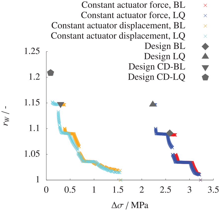
Figure 12 compares the resulting Pareto fronts. It is noticeable that the use of actuators with constant displacements leads to a tremendous reduction of the stress difference $Δ σ$ without increasing the actuation effort $r_{W}$ . This applies to both definitions of the border thickness. Besides that, it is visible, that a varying border thickness also has a positive effect when using actuators of constant displacement.

Figure 12.

Pareto fronts obtained with actuators of constant force using linear + quadratic thickness distribution (LQ) and constant displacement using constant border thickness (BL) as well as linear + quadratic thickness distribution (LQ).

Details of the design with minimal stress difference using actuators of constant displacement and a constant border thickness (CD-BL, see Figure A5 in the Appendix) confirms this observation. The stress is homogenized over the measuring region, compared to the baseline result (BL, see Figure 9). Nevertheless, an undesired shearing is still observed in the outer corner.

This undesired effect is overcome by the corresponding design enhanced by the linear and quadratic border thickness variation (CD-LQ, see Figure A6 in the Appendix). It shows a remarkable use of the design freedom of the border region thickness definition. Again, the thickness is linearly increased toward the actuator region. In contrast to the solution with actuators of constant force (LQ, Figure A4), the thickness along the specimen edges is increased quadratically toward the specimen corner. By that, a stiffening of the border corner is obtained. With actuators of constant displacement, shearing of the measuring region is nevertheless avoided by an implicit load shifting of the actuators. This leads to an almost perfectly homogeneous biaxial stress state, as shown in Figure A6 in the Appendix. Quantitative details of the designs CD-BL and CD-LQ are summarized in Table A1.

Homogeneity of equivalent stress distribution

The final analysis of the achieved homogeneity of the equivalent stress distribution in the measuring region allows the practical quantification and evaluation of the benefit of different design characteristics for biaxial tensile tests.

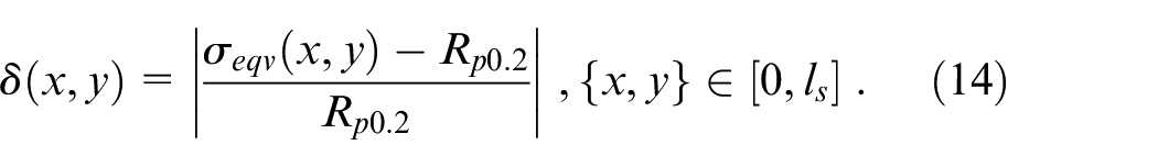
One of the main targets of biaxial tensile tests for determining the contour of elastic deformation is to reach the 0.2% proof stress over a measuring region as large as possible. This results in an homogeneous stress state and avoids undesired stress artifacts. In order to compare the homogeneity of the equivalent stress distribution $σ_{eqv} (x, y)$ in the measuring region, the relative stress difference to the 0.2% proof stress is considered:

δ (x, y) = | \frac{σ_{eqv} (x, y) - R_{p 0.2}}{R_{p 0.2}} |, {x, y} \in [0, l_{s}] .

(14)

The histogram in Figure 13 shows the area ratio $A (δ_{\max}) / A_{res}$ of the total area of the measuring region $A_{res} = l_{s}^{2}$ over the upper boundary of the relative stress difference $δ_{\max}$ . Hereby, $A (δ_{\max})$ is defined as the area where the relative error $δ (x, y)$ according to equation (14) does not exceed the maximum value $δ_{\max}$ :

\begin{matrix} A (δ_{\max}) = \int_{x = 0}^{l_{s}} \int_{y = 0}^{l_{s}} g (x, y, δ_{\max}) d x d y with \\ g (x, y, δ_{\max}) = {\begin{matrix} 1 & if δ (x, y) \leq δ_{\max} \\ 0 & other wise \end{matrix} . \end{matrix}

(15)

Figure 13.

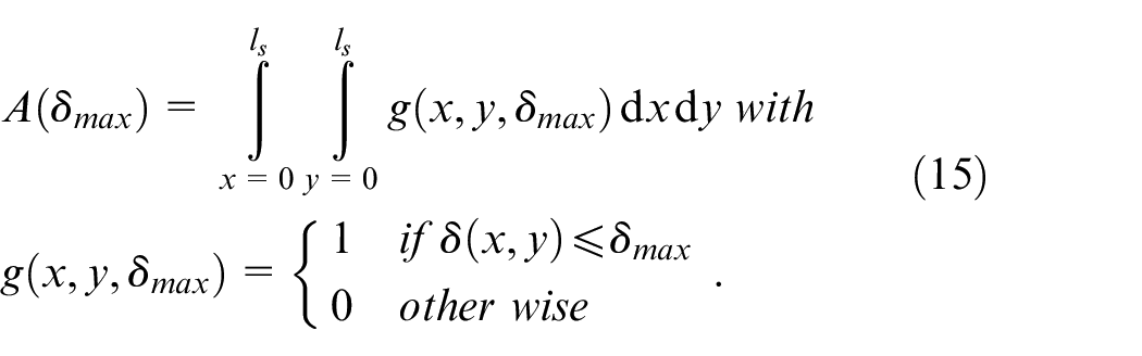
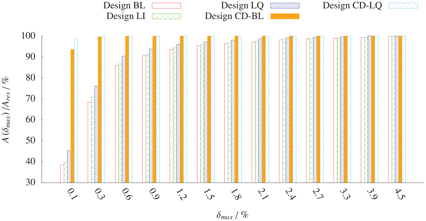
Histograms of the ratio $A (δ_{\max}) / A_{res}$ of the measuring region over the upper limit $δ_{\max}$ for the relative error between the equivalent stress $σ_{eqv}$ and the 0.2% proof stress $R_{p 0.2}$ for the designs with minimal stress difference $Δ σ$ .

By that, intuitive quantitative analyses of the benefits of the different design characteristics are possible.

In accordance to the results discussed before, the homogeneity can be greatly influenced by specific border topographies. The linear thickness variation allows a slight improvement with an error not exceeding 0.1% over 39.9% of the region, compared to 38.5% of the region with a constant border thickness. In explicit, considering $δ_{m a x} = 0.1 %$ , the homogeneity has been widened by $1.4$ percentage points of the region by the linear thickness distribution. A more significant improvement is possible by adding the quadratic thickness distribution. Here, 45.3% of the measuring region reach an relative error below 0.1%. In contrast to the linear thickness distribution, the relevant region has further been enlarged by $5.4$ percentage points, resulting in a better homogeneity of the equivalent stress distribution. This effect is also visible when comparing Figure A4(f) and Figure A3(f). The main driver for this effect is the reduction of the undesired shearing at the outer specimen corners, resulting from the coupling of both loading directions. It is noticeable that the shear stress effects the equivalent stress by a factor of three (see equation (1)). Therefore, the reduction of the undesired shearing has a higher influence on $δ$ , compared to the reduction of discontinuities of the normal stresses which can already be achieved by the linear thickness variation.

Finally, using an actuation with constant displacements improves significantly the homogeneity. In combination with a constant border thickness, a maximum relative error of 0.1% can be obtained over 93.6%. Also in this case, refining the border topography by a linear and quadratic distribution allows to further minimize stress concentrations. With this, an almost perfectly homogeneous stress state with $δ_{m a x} = 0.1 %$ over 98.8% of the measuring region can be maintained, as Figure A6(f) shows.

Deduction of design proposals

The comprehensive discussion of the optimization results allows the deduction of general design proposals for biaxial tensile test specimens for obtaining the target principal stress state $σ_{x, ref} = σ_{y, ref} = R_{p 0.2}$ , $τ_{xy, ref} = 0$ .

Regarding the thickness definition of the border region and the load introduction, the following aspects shall be taken into account:

Load application shall be ensured over the full length of the border region edges.

The number of discrete elements for load introduction shall be as large as possible, in order to constrain lateral strain as less as possible. Furthermore, the gaps between discrete load introduction elements shall be as small as possible. Hence, the theoretical optimum would be a load introduction of an infinite number of filaments with infinite dense placement along the border region edges.

A linear thickness distribution of the border region between the edges of the measuring region and the load introduction is beneficial. The thickness should be increased toward the load introduction region. By that, stress concentrations arising from the load introduction can be kept in the border region and stiffness discontinuities at the edges of the measuring region are minimized.

Further significant improvement of the homogeneity of the equivalent stress is possible by a quadratic thickness variation of the border region parallel to the specimen edges. If the actuation ensures a constant force along each specimen edge, the thickness shall be reduced toward the specimen corners. On the other hand, the thickness shall be increased toward the specimen corners if a displacement-constant actuation is chosen.

Load introduction with constant displacements along each specimen edge allows a significant reduction of the stress difference, compared to an actuation of constant force. After choosing one of these two types, the thickness distribution of the border region shall be defined according to aspect IV.

Conclusion and outlook

The present paper deals with the multi-objective optimization of a biaxial tensile test specimen with the objectives of minimizing the stress difference to the target principal stress state $σ_{x, ref} = σ_{y, ref} = R_{p 0.2}$ , $τ_{xy, ref} = 0$ and the actuation effort.

The chosen structural parameterization allows a high degree of freedom where emphasis has been put on allowing sensible and target-orientated thickness definitions of the border region. Concerning the load introduction, actuation with constant force and constant displacement has been considered. The optimization approach allows a well-founded quantification of the influence of the investigated design characteristics.

A detailed discussion of the obtained results allowed the deduction of design proposals. These state that a linear thickness variation of the border region between the edges of the measuring region and the load introduction allows to better match the desired target stress state, compared to a constantly thickened border region. Additional benefits are gained by a quadratic variation of the border thickness along the specimen edges. Especially, the homogeneity of the equivalent stress distribution can be greatly improved by allowing a quadratic thickness distribution along the border edges. When using a border region, it should include the specimen corners. In this case, they should be used for load introduction. Finally, constant displacement actuators are superior to actuators of constant force, as the implicit load shifting minimizes undesired shearing of the measuring region. Nevertheless, also in the case of constant displacement actuators, the refined border topography with a linear and quadratic thickness variation is beneficial.

For practical application, these design proposals have to be carefully chosen based on an effort-benefit comparison. For that, the present optimization approach as well as the obtained results and the stress histogram provide a valuable basis. With this, it is possible to quantify the effect of designs of varying sophistication and perform a well-founded decision.

Further research will be done in order to include multiple target stress states in the optimization process. This will allow design proposals of test specimens intended for a best compromise representation of several target stress states, for example in order to represent a full yield strength curve. Besides that, more refined investigations regarding the topology and thickness distribution of the border region will be performed. Furthermore, generalization to other target stress states, as well as modifications for taking orthotropic materials into account, is projected.

Footnotes

Appendix

Table A1.

Characteristic values of the selected designs.

Description	Variable	Unit	Design
			Constant force					Constant displacement
			BL	ME	CM	LI	LQ	CD-BL	CD-LQ
Numbers of actuators per half-length of the specimen	$n_{act}$	-	11	11	11	11	11	11	11
Border width	$w_{b}$	mm	4.6396	0.1001	1.7677	7.2500	7.2500	7.2500	9.9714
Actuator width	$w_{act}$	mm	5.0000	5.0000	5.0000	5.0000	5.0000	5.0000	5.0000
Line force	$q_{act}$	N/mm	274.58	273.48	274.02	274.44	274.42	281.18	282.25
Border thickness 0	$t_{b, 0}$	mm	1.1843	1.3120	1.2031	1.2168	1.2243	1.1903	1.2257
Border thickness 1	$t_{b, 1}$	mm	1.1843	1.3120	1.2031	1.2168	1.1256	1.1903	1.2961
Border thickness 2	$t_{b, 2}$	mm	1.1843	1.3120	1.2031	1.0000	1.0000	1.1903	1.0000
Actuator thickness	$t_{act}$	mm	2.1559	2.1793	2.1720	2.1451	2.1443	5.4978	6.4925
Stress difference	$Δ σ$	MPa	2.5853	3.2302	2.7594	2.3156	2.2300	0.2993	0.0904
Total strain energy ratio	$r_{W}$	-	1.0912	1.0000	1.0352	1.1460	1.1467	1.1481	1.2086

Acknowledgements

We thank Mr. Mirko Sachse and Dr. Silvio Nebel from IMA Materialforschung und Anwendungs-technik GmbH in Dresden for fruitful discussions of practical aspects of biaxial tensile tests. Calculations have been performed on the Bull HPC-cluster of the Zentrum für Informationsdienste und Hochleistungs-rechnen (ZIH) of the Technische Universität Dresden.

Declaration of conflicting interests

The author(s) declared no potential conflicts of interest with respect to the research, authorship, and/or publication of this article.

Funding

The author(s) disclosed receipt of the following financial support for the research, authorship, and/or publication of this article: This research was funded by the German Federal Ministry for Economic Affairs and Climate Action under grant number 20Q1716B. The responsibility for the content of this paper is with its authors. The financial support is gratefully acknowledged.

ORCID iD

Florian Dexl

References

Hannon

Tiernan

A review of planar biaxial tensile test systems for sheet metal. J Mater Process Technol 2008; 198(1–3): 1–13.

Abu-Farha

Hector

Khraisheh

Cruciform-shaped specimens for elevated temperature biaxial testing of lightweight materials. JOM 2009; 61(8): 48–56.

Kuwabara

Advances in experiments on metal sheets and tubes in support of constitutive modeling and forming simulations. Int J Plast 2007; 23(3): 385–419.

Xiao

A review of cruciform biaxial tensile testing of sheet metals. Exp Tech 2019; 43(5): 501–520.

Demmerle

Boehler

JP.

Optimal design of biaxial tensile cruciform specimens. J Mech Phys Solids 1993; 41(1): 143–181.

Zhu

Zhang

, et al. Optimal design of a miniaturized cruciform specimen for biaxial testing of TA2 alloys. Metals 2019; 9(8): 823.

Nasdala

Husni

AH.

Determination of yield surfaces in accordance with ISO 16842 using an optimized cruciform test specimen. Exp Mech 2020; 60(6): 815–832.

Zhao

Chen

Xiao

, et al. Design of a biaxial tensile testing device and cruciform specimens for large plastic deformation in the central zone. J Mater Sci 2019; 54(9): 7231–7245.

Makris

Vandenbergh

Ramault

, et al. Shape optimisation of a biaxially loaded cruciform specimen. Polym Test 2010; 29(2): 216–223.

10.

Bauer

Priesnitz

Schemmann

, et al. Parametric shape optimization of biaxial tensile specimen. Proc Appl Math Mech 2016; 16(1): 159–160.

11.

Yang

, et al. Optimization design of cruciform specimens for biaxial testing based on genetic algorithm. J Mater Eng Perform 2022. DOI: 10.1007/s11665-022-07258-6

12.

Andrusca

Goanta

Barsanescu

PD.

Optimizing the shape and size of cruciform specimens used for biaxial tensile test. Appl Mech Mater 2014; 658: 167–172.

13.

Andrusca

Goanta

Barsanescu

, et al. Numerical and experimental study of cruciform specimens subjected to biaxial tensile test. IOP Conf Ser Mater Sci Eng 2016; 147: 012091.

14.

Xiao

Lang

, et al. Design of biaxial tensile cruciform specimen based on simulation optimization. In: Proceedings of the 2015 2nd international conference on machinery, materials engineering, chemical engineering and biotechnology, pp.178–186. Chongqing: Atlantis Press. DOI: 10.2991/mmeceb-15.2016.37.

15.

Shao

Lin

The optimisation of cruciform specimen for the formability evaluation of AA6082 under hot stamping conditions. Procedia Eng 2017; 207: 735–740.

16.

Liedmann

Gerke

Barthold

, et al. Shape optimization of the x0-specimen: theory, numerical simulation and experimental verification. Comput Mech 2020; 66(6): 1275–1291.

17.

Liedmann

Barthold

FJ.

Variational sensitivity analysis of elastoplastic structures applied to optimal shape of specimens. Struct Multidiscipl Optim 2020; 61(6): 2237–2251.

18.

Hanabusa

Takizawa

Kuwabara

Numerical verification of a biaxial tensile test method using a cruciform specimen. J Mater Process Technol 2013; 213(6): 961–970.

19.

Hartmann

Gilbert

Sguazzo

Basic studies in biaxial tensile tests. GAMM-Mitt 2018; 41(1): e201800004.

20.

Lang

Schemmann

Seelig

, et al. Investigations of cruciform specimen designs for biaxial tensile testing of SMC. Proceedings 2018; 2(8): 411.

21.

Schemmann

Lang

Helfrich

, et al. Cruciform specimen design for biaxial tensile testing of SMC. J Compos Sci 2018; 2(1): 12.

22.

Hou

Min

Lin

, et al. Cruciform specimen design for large plastic strain during biaxial tensile testing. J Phys Conf Ser 2018; 1063: 012160.

23.

Kaletta

Ein Beitrag zur Effizienzsteigerung Evolutionärer Algorithmen zur optimalen Auslegung von Faserverbundstrukturen im Flugzeugbau. PhD Thesis, Technische Universität Dresden, Dresden, 2006.

24.

Seeger

Wolf

Multi-objective design of complex aircraft structures using evolutionary algorithms. Proc IMechE, Part G: J Aerospace Engineering 2011; 225(10): 1153–1164.

25.

Seeger

Ein Beitrag zur numerischen Strukturauslegung aktiver Rotorblätter unter Berücksichtigung der Wechselwirkung von Strömung und Struktur. PhD Thesis, Technische Universität Dresden, Dresden, 2012.

26.

Machunze

Gessler

Fabel

, et al. Active flow control system integration into a CFRP flap. CEAS Aeronaut J 2016; 7(1): 69–81.

27.

Dexl

Hauffe

Wolf

Multidisciplinary multi-objective design optimization of an active morphing wing section. Struct Multidiscipl Optim 2020; 62(5): 2423–2440.

Numerical optimization-based design studies on biaxial tensile tests

Abstract

Keywords

Introduction

Problem definition and basic assumptions

Aims and limitations

Target stress state

General outline of the test specimen geometry

Planes of symmetry

Load introduction

Thicknesses

Optimization framework

Parametric model

Optimization problem

Evolutionary optimization

Structural evaluation and Finite Element model

Results

Baseline design

Influence of border thickness definition

Influence of actuators with constant displacement

Homogeneity of equivalent stress distribution

Deduction of design proposals

Conclusion and outlook

Footnotes

Appendix

Acknowledgements

Declaration of conflicting interests

Funding

ORCID iD

References