Sage Journals: Discover world-class research

Abstract

The specimen strain rate in the split Hopkinson bar (SHB) test has been formulated based on a one-dimensional assumption. The strain rate is found to be controlled by the stress and strain of the deforming specimen, geometry (the length and diameter) of specimen, impedance of bar, and impact velocity. The specimen strain rate evolves as a result of the competition between the rate-increasing and rate-decreasing factors. Unless the two factors are balanced, the specimen strain rate generally varies (decreases or increases) with strain (specimen deformation), which is the physical origin of the varying nature of the specimen strain rate in the SHB test. According to the formulated strain rate equation, the curves of stress–strain and strain rate–strain are mutually correlated. Based on the correlation of these curves, the strain rate equation is verified through a numerical simulation and experiment. The formulated equation can be used as a tool for verifying the measured strain rate–strain curve simultaneously with the measured stress–strain curve. A practical method for predicting the specimen strain rate before carrying out the SHB test has also been presented. The method simultaneously solves the formulated strain rate equation and a reasonably estimated constitutive equation of specimen to generate the anticipated curves of strain rate–strain and stress–strain in the SHB test. An Excel® program to solve the two equations is provided. The strain rate equation also indicates that the increase in specimen stress during deformation (e.g., work hardening) plays a role in decreasing the slope of the strain rate–strain curve in the plastic regime. However, according to the strain rate equation, the slope of the strain rate–strain curve in the plastic deformation regime can be tailored by controlling the specimen diameter. Two practical methods for determining the specimen diameter to achieve a nearly constant strain rate are presented.

Keywords

Elasto-plastic modelling impact mechanics prediction model material mechanical properties

Introduction

High-strain-rate events, such as crashes of high-speed transportation means (automobiles, airplanes, and express trains), high-speed machining, rock/building blasting, explosive welding, meteorite impact, projectile penetration, explosion, and blast impact, need an in-depth understanding of physics behind the events to achieve a reliable design of solids and structures associated with the events. Relying solely on experimental approaches for the design/understanding of the high-strain-rate behaviour of solids and structures may not be practical because of the burden of cost and time; however, an experimental verification of the design result is inevitable. Modelling and simulation (M & S)^1–7 helps one to understand the evolution of the high-strain-rate phenomena on a step-by-step basis and is a time- and cost-efficient design approach. Therefore, it is advantageous to combine the M & S-based design with experimental verification of the mechanical behaviour of solids and structures exposed to high-strain-rate events.

For the M & S-based design/understanding of the high-strain-rate behaviour of solids and structures, a strain rate-dependent constitutive model^8–11 is indispensable (together with the fracture model and equation of state, if necessary). A number of uniaxial stress–strain curves measured precisely at a wide range of strain rates^12–23 are required for the calibration of the strain rate-dependent constitutive model.

The split Hopkinson bar (SHB),^24,25 which is also called the Kolsky bar, has been used extensively for measuring the uniaxial stress–strain curves of various materials at high strain rates (10² to 10⁴ s⁻¹). The fundamental theory and applications of SHB are well described in the literature (books^26–29 and review papers^30–34). The SHB is used to determine the dynamic stress–strain curves of not only metals^12–23 but also non-metallic materials^35–45 such as ceramics, concrete, rocks, soil (sand), plastics, rubber, foam, honeycombs, wood, and various types of composites.

In the SHB test, the reflected pulse monitored in the input bar represents the specimen strain rate.^25–34 Despite the fluctuating nature of pulses in the elastic bar, the magnitude of the reflected pulse (the strain rate) often decreases/increases significantly with time (with specimen deformation).^46–50 For the maximal utilisation of the SHB, it is necessary to understand the varying nature (evolution) of the specimen strain rate in the SHB test from the viewpoint of mechanical science. Such fundamental understanding may lead to finding practical means of solving issues to be cleared in the SHB test, which will be described in the succeeding paragraphs. In the literature, however, the physical origin of the varying nature of the specimen strain rate in the SHB test has not been well studied. In this regard, the primary, and probably the most important, purpose of this study is to find out the physical origin of the varying nature of specimen strain rate in the SHB test. For this purpose, this study formulates the evolution of specimen strain rate in the SHB test as a function of the specimen strain. The formulation process is presented in the Formulation of strain rate equation section. The physical origin of the varying nature of specimen strain rate in the SHB test will be presented using the formulated strain rate equation.

In the literature, the reliability of the measured stress–strain curve has been verified by checking the coincidence of stresses at the front and back surfaces of the specimen (stress equilibrium).^49–56 However, as for the reliability of the strain rate–strain curve of specimen, which is also required for the calibration of a strain rate-dependent constitutive model, there has been no direct tool to verify the measured result. If a method for verifying the measured strain rate–strain curve is available, it can also be verified, improving the reliability of the SHB test. In this regard, the second purpose of this study is to present a method for verifying the measured strain rate–strain curve simultaneously with the measured stress–strain curve using the formulated strain rate equation based on the correlation of the strain rate–strain curve with the stress–strain curve; the strain rate equation describes the relationship between the two curves.

In the SHB test, the unknown stress–strain curve of the specimen is determined at a target strain rate. The issue is that the specimen strain rate is also unknown. The state-of-the-art technology to obtain the target strain rate in the SHB test relies on trials or previous experience. The actually manifested specimen strain rate in the SHB test can be revealed only after the experiment is finished. In the literature, it is difficult to find a method for predicting the specimen strain rate before carrying out the SHB test. If a method for predicting the specimen strain rate is available, it should be useful for the design of the experiment. In this regard, the third purpose of this study is to present a practical method for predicting the specimen strain rate before carrying out the SHB test: the method simultaneously solves the formulated strain rate equation and a reasonably estimated constitutive equation of the specimen, which results in the anticipated curves of strain rate–strain and stress–strain in the SHB test. An Excel® program for solving the two equations is provided in the Supplemental Material.

The fourth purpose of this study is to present a method for predicting the maximum specimen strain in the SHB test, which is also unavailable in the current technology. To predict the maximum specimen strain, the presented method combines the strain rate–strain curve with the pulse duration time. Such an algorithm is also included in the Excel® program.

As mentioned, the specimen strain rate usually varies during the SHB test. From the viewpoint of measuring the material properties or investigating a dynamic phenomenon at a given strain rate, it is necessary to control the specimen strain rate in the SHB test to achieve a constant strain rate. In this regard, researchers employed the pulse shaping techniques,^28,57–65 that utilise a conical striker, dummy specimen, or tip material to obtain a nearly constant strain rate. The achieved nearly constant strain rate using these techniques can be confirmed from the result of numerical analyses. However, a theory-based understanding of the achieved result using the above-mentioned techniques is limited because there are no analytical expressions describing the reason for achieving a nearly constant strain rate available. The process of achieving a nearly constant strain rate in these techniques is an iterative process based on an open loop control,²⁸ which means that the iteration process does not need the feedback of the previous result. The conditions for achieving a nearly constant strain rate depend on the unknown properties of the specimen to be tested such as the dynamic stress–strain curve. The conditions of the constant strain rate also depend on the impact velocity and specimen geometry. The reason for such dependencies of the constant-strain-rate conditions in the pulse shaping techniques is currently unavailable. If a theory-based method for achieving a nearly constant strain rate in the standard SHB test (without the aid of the pulse shaper or conical striker) is available, the method will allow researchers to readily understand why a nearly constant strain rate was achieved in their test and may serve as an informative method for achieving a nearly constant strain rate. In this regard, this study finally aims at presenting a theory-based method for tailoring the slope of the strain rate–strain curve based on the formulated strain rate equation by simply controlling the specimen diameter. Two practical methods to determine the specimen diameter for achieving a nearly constant strain rate are presented.

In this study, the term ‘rate’ means the ‘strain rate’ hereafter. The term ‘rate–strain curve’ will be used preferably to the term ‘strain rate–strain curve’ for improving readability. The term ‘rate equation’ is used interchangeably with the term ‘strain rate equation’.

Formulation of strain rate equation

Assumptions

This study employs the same assumptions as those of the fundamental (one-dimensional) theory of SHB^25–34:

The velocity of the elastic wave in the bars is described by a slender rod (one-dimensional) approximation (C_o = (E_o/ρ_o)^1/2).

The specimen expands freely along the radial direction (no friction between the specimen and the bars) while it deforms axially.

There is no inertia in the specimen and bars.

The specimen deforms uniformly along the axial direction; the stress and strain of the specimen at the front surface of the specimen are the same as those at the rear surface of the specimen; this stress uniformity of the specimen results in the force equilibrium between the ends of the bars, which are in contact with the specimen.

Formulation

This study considers the compression-mode SHB following the original inception of the SHB. Figure 1 schematically illustrates the sign convention employed in this study for the compression-mode SHB: a positive sign is assigned to the compressive property and left-travelling direction. As can be observed in Figure 1, the signs of the stress (strain) and particle velocity are the same for the left-travelling wave (reflected pulse) while they are opposite to each other for the right-travelling wave (incident and transmitted pulses).

Figure 1.

Sign convention for the compression-mode SHB, which is employed in this study. A positive sign is assigned to the compressive property and left-travelling direction. The numbers 1 and 2 denote the end surfaces of the input bar and output bar, respectively. The profile of the pulse is concave for compression and convex for tension.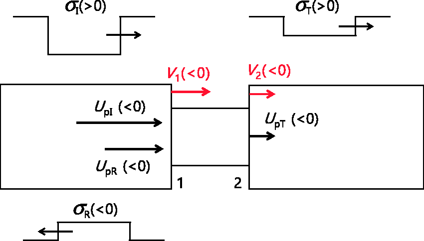

The average (engineering) strain rate of a deforming specimen in the compression-mode SHB is given by

\begin{matrix} \overset{\cdot}{e} = de / dt = - [V_{1} (t) - V_{2} (t)] / L \end{matrix}

(1)

The rate of the true strain is expressed as

\overset{\cdot}{ɛ} = d ɛ / dt = - [V_{1} (t) - V_{2} (t)] / L_{c}

(2)

This study pursues an analytical formulation of the strain rate in a closed form by expressing V₁ and V₂ in terms of the specimen stress and substituting them into equation (1) or (2). Here, V₂ is formulated first, followed by V₁.

V₂ at a given moment during specimen deformation is^25–34

V_{2} = U_{p 2} = - σ_{2} / ρ_{o} C_{o} = - A_{c} σ / A_{o} ρ_{o} C_{o}

(3)

where U_p2 is the particle velocity at the output bar, σ₂ is the stress at the output bar, A_c is the current cross-sectional area of the specimen, and σ is the true stress of the specimen. In equation (3), a negative sign appears between the stress and particle velocity because U_p2 ( = –σ₂/ρ_oC_o) is for the right-travelling wave (σ₂ is positive).

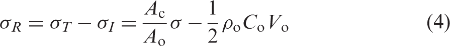
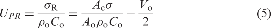
To develop the expression for V₁, it is assumed that a force equilibrium between the bars (F₁ = F₂; σ_I+σ_R = σ_T) is achieved. Then, σ_R ( < 0) is

\begin{matrix} σ_{R} = σ_{T} - σ_{I} = \frac{A_{c}}{A_{o}} σ - \frac{1}{2} ρ_{o} C_{o} V_{o} \end{matrix}

(4)

In equation (4), the relationship for σ_I ( = ρ_oC_oV_o/2) results from the momentum conservation between the striker and the input bar.²⁷ Here, V_o is set as positive. Because the reflected pulse is a left-travelling wave, the signs of U_pR and σ_R are the same:

\begin{matrix} U_{PR} = \frac{σ_{R}}{ρ_{o} C_{o}} = \frac{A_{c} σ}{A_{o} ρ_{o} C_{o}} - \frac{V_{o}}{2} \end{matrix}

(5)

In equation (5), the expression for σ_R in equation (4) is applied. The expression for V₁ ( = U_pI+U_pR; U_pI = –V_o/2²⁷) is given by

\begin{matrix} V_{1} = U_{pI} + U_{pR} = - V_{o} + A_{c} σ / A_{o} ρ_{o} C_{o} \end{matrix}

(6)

By substituting V₁ and V₂ into equation (2), the rate of the true strain ( $\overset{\cdot}{ɛ}$ ) of the deforming specimen is obtained as

\begin{matrix} \overset{\cdot}{ɛ} = \frac{1}{L_{c}} (V_{o} - \frac{2 A_{c} σ}{A_{o} ρ_{o} C_{o}}) \end{matrix}

(7)

From the assumption of incompressibility of a uniformly deforming specimen, i.e. A_cL_c = AL, the following relationships are established

L_{c} = L exp (- ɛ)

(8)

A_{c} = A / exp (- ɛ)

(9)

where L_c < L and A_c > A in compression (ɛ is positive). By applying these relationships to equation (7), the rate of the true strain of the deforming specimen is obtained as

\begin{matrix} \overset{\cdot}{ɛ} = \frac{1}{L exp (- ɛ)} (V_{o} - \frac{2 A}{A_{o} ρ_{o} C_{o} exp (- ɛ)} σ) \end{matrix}

(10)

Equation (10) is the strain rate equation (or simply the rate equation) referred in this study.

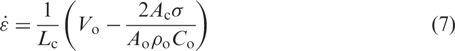
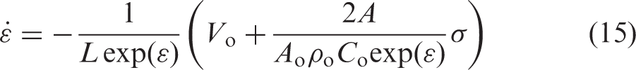
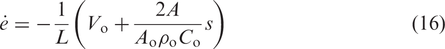
The rate of the engineering strain ( $\overset{\cdot}{e}$ ) of the deforming specimen is obtained by substituting V₁ (equation (6)) and V₂ (equation (3)) into equation (1):

\overset{\cdot}{e} = \frac{1}{L} (V_{o} - \frac{2 A_{c} σ}{A_{o} ρ_{o} C_{o}})

(11)

A_c and σ in equation (11) can be expressed in terms of engineering properties (e is positive)

A_{c} = A / (1 - e)

(12)

σ = s (1 - e)

(13)

Then, the rate of engineering strain is

\overset{\cdot}{e} = \frac{1}{L} (V_{o} - \frac{2 A}{A_{o} ρ_{o} C_{o}} s)

(14)

In the final rate equations (equations (10) and (14)) for the compression-mode SHB, the sign of σ, s, ɛ, e,

\overset{\cdot}{ɛ}

, and

\overset{\cdot}{e}

is positive (V_o is set as positive).

If a positive sign is assigned to the tensile property and right-travelling direction for the compression-mode SHB (Figure 2), the rate equations are

\overset{\cdot}{ɛ} = - \frac{1}{L exp (ɛ)} (V_{o} + \frac{2 A}{A_{o} ρ_{o} C_{o} exp (ɛ)} σ)

(15)

\overset{\cdot}{e} = - \frac{1}{L} (V_{o} + \frac{2 A}{A_{o} ρ_{o} C_{o}} s)

(16)

In the above equations, σ, s, ɛ, e,

\overset{\cdot}{ɛ}

, and

\overset{\cdot}{e}

are negative (V_o is set as positive).

Figure 2.

Sign convention for the compression-mode SHB when a positive sign is assigned to the tensile property and right-travelling direction. The profile of the pulse is concave for compression and convex for tension.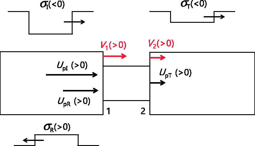

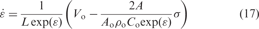
For the tension-mode SHB, a positive sign is generally assigned to the tensile property and right-travelling direction (Figure 3). In such a case, the rate equations are

\begin{matrix} \overset{\cdot}{ɛ} = \frac{1}{L exp (ɛ)} (V_{o} - \frac{2 A}{A_{o} ρ_{o} C_{o} exp (ɛ)} σ) \end{matrix}

(17)

\overset{\cdot}{e} = \frac{1}{L} (V_{o} - \frac{2 A}{A_{o} ρ_{o} C_{o}} s)

(18)

In the above equations, σ, s, ɛ, e,

\overset{\cdot}{ɛ}

, and

\overset{\cdot}{e}

are positive (V_o is set as positive).

Figure 3.

Sign convention for the tension-mode SHB. A positive sign is assigned to the tensile property and right-travelling direction. The profile of the pulse is concave for compression and convex for tension.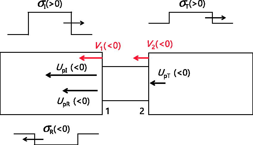

Methods

Numerical simulation

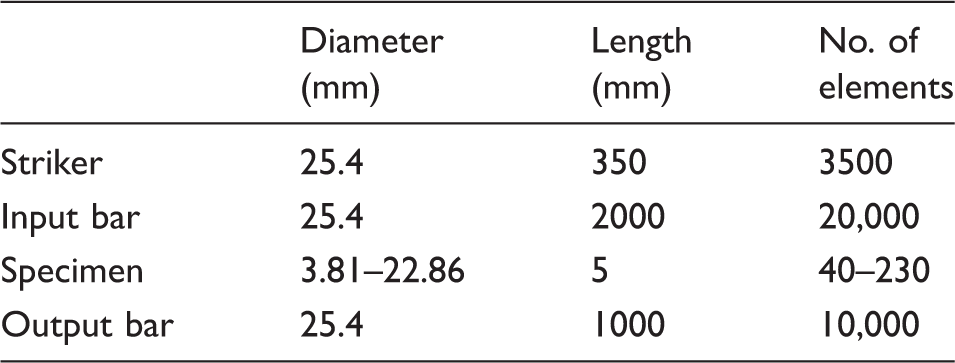
The SHB experiment was simulated via an explicit finite element analysis. Considering the axial symmetry of the SHB system, only half of the two-dimensional axi-symmetric geometry was discretised using four-node bilinear axi-symmetric quadrilateral elements. No friction was considered between the contact surfaces. The number of elements in each section of the discretised region is listed in Table 1. These elements passed a mesh sensitivity test, which was carried out separately.

Table 1.

Dimensions of SHB system considered in the numerical simulation and number of elements in the finite element model.

	Diameter (mm)	Length (mm)	No. of elements
Striker	25.4	350	3500
Input bar	25.4	2000	20,000
Specimen	3.81–22.86	5	40–230
Output bar	25.4	1000	10,000

The flow stress of specimen material was described using the Johnson–Cook (JC) constitutive model:⁸

\begin{matrix} σ^{pl} = [a + b ɛ^{n}] [1 + c \ln (\frac{\overset{\cdot}{ɛ}}{{\overset{\cdot}{ɛ}}_{o}})] [1 - (\frac{T - T_{ref}}{T_{m} - T_{ref}}) m] \end{matrix}

(19)

The properties of the materials used for the numerical simulation are given in Tables 2 and 3. Copper is considered in this study as the specimen material unless otherwise specified; it is one of the representative work-hardening materials and has been tested extensively using the standard SHB instrument.

Table 2.

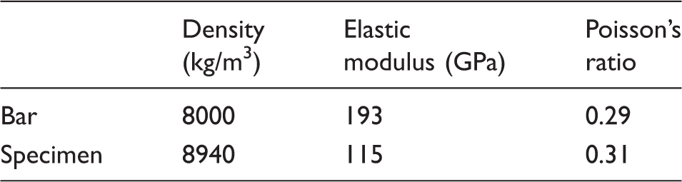
Density and elastic properties of the annealed OFHC copper specimen and bar considered in the numerical simulation.

	Density (kg/m³)	Elastic modulus (GPa)	Poisson's ratio
Bar	8000	193	0.29
Specimen	8940	115	0.31

Table 3.

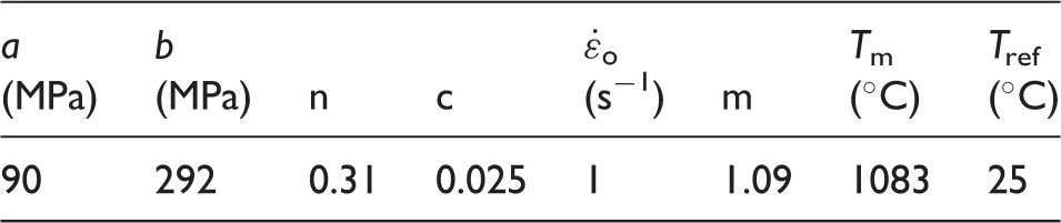
Constitutive parameters of the JC model for annealed OFHC copper⁸

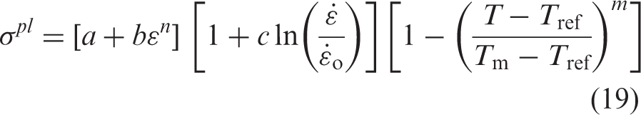
a (MPa)	b (MPa)	n	c	${\overset{\cdot}{ɛ}}_{o}$ (s⁻¹)	m	T_m (℃)	T_ref (℃)
90	292	0.31	0.025	1	1.09	1083	25

This study first considered the case where the specimen property is independent of the strain rate and temperature (simulation case 1); only the first bracket in equation (19) was used to describe the flow stress. Then, the case where the flow stress of the specimen is dependent on the strain rate and temperature (simulation case 2) was considered; all three brackets in equation (19) were considered. For such a purpose, the specimen was assumed to deform adiabatically. For adiabatic deformation, a specific heat value of 383 Jkg⁻¹K⁻¹ was set and 90% of the plastic work was assumed to be converted to heat.

The striker travelled at a constant velocity until it impacted onto the input bar, which was 1 mm away. Two different impact velocities (10 or 20 m/s) were considered in the numerical simulation (the impact velocity is specified when presenting the simulation result later). A commercial finite element package, ABAQUS/Explicit,⁶⁶ was used as the solver.

In the post-processing of numerical analysis, the bar signals, $e_{R} (t)$ and $e_{T} (t)$ , were extracted by averaging the true strains of two elements (sensor elements) at the surfaces of the input and output bars, respectively. The sensor elements at each bar were located at distances of 1000 and 300 mm, respectively, from the specimen. Curves of engineering stress–strain and engineering rate–strain were determined (measured) using the bar signals ( $e_{R} (t)$ and $e_{T} (t)$ ; pulse records) via a one-wave analysis of the SHB theory:^25–34

\begin{matrix} s = \frac{A_{o}}{A} E_{o} e_{T} (t) \end{matrix}

(20)

\begin{matrix} \overset{\cdot}{e} = - \frac{2 C_{o}}{L} e_{R} (t) \end{matrix}

(21)

\begin{matrix} e = - \frac{2 C_{o}}{L} \int_{o}^{t} e_{R} (t) d t \end{matrix}

(22)

Experiment

The as-received oxygen-free copper (OFC) specimen was machined to have relative diameters (D/D_o) of 0.7, 0.4, and 0.2 at a nominal thickness of 5 mm. The machined specimen was annealed at 600℃ for 2 h in flowing N₂–10%H₂ atmosphere. The flow rate was 1 L/min in an alumina tube with 60 mm in inner diameter. The top/bottom surfaces of the specimens were polished using diamond pastes with 15, 6, 3, and 1 μm in average particle diameter (in sequence). The final geometry of the specimens is presented in Table 4.

Table 4.

Specimen geometry and impact velocity in the SHB experiment.

D/D_o	0.7	0.4	0.2
D (mm)	17.83	10.17	5.11
L (mm)	5.04	4.98	5.02
V_o (m/s)	10.06	10.70	10.06

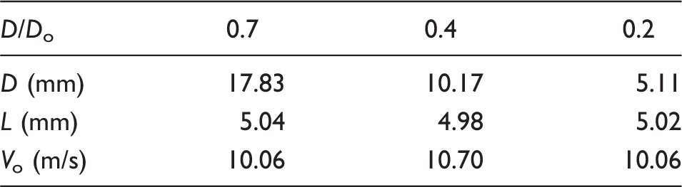
The SHB system used in this study was made of maraging steel. The dimensions of the SHB system used in the experiment were the same as the dimensions considered for the numerical simulation (Table 1). An aliquot of lubricant was applied at the contact surfaces between the bars and specimen. No pulse shaper was used intentionally as this study focuses on the standard SHB. The SHB testing of the specimens was carried out at a nominal impact velocity of 10 m/s (detailed impact velocities are listed in Table 4) at ambient temperature.

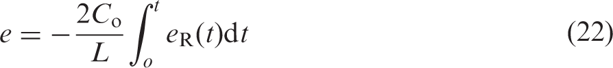
The curves of engineering stress–strain and engineering rate–strain were measured by treating the bar signals via one-wave analysis (equations (20) to (22)). They were converted to curves of true stress–strain and true rate–strain by assuming that the specimen is incompressible (at Poisson's ratio of 0.5) and deforms uniformly although, in the elastic regime, the specimen is compressible according to the Poisson's ratio of 0.31 (Table 1). This limitation exists only in the elastic part of deformation because the plastic deformation of a metallic specimen is incompressible. The same conversion process was applied as well in obtaining the curves for the true stress–strain and true rate–strain from the engineering properties in the post-processing of numerical analysis.

Results and discussion

Numerical verification of rate equation

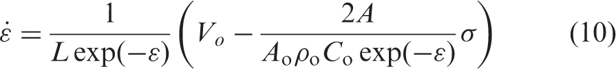
The formulated strain rate equation (equation (10)) indicates that if the stress (σ) of the specimen at a given strain (ɛ) is known, the strain rate ( $\overset{\cdot}{ɛ}$ ) at the given strain (ɛ) can be determined: an (ɛ, σ) data point can be converted to an (ɛ, $\overset{\cdot}{ɛ}$ ) data point via the rate equation. In other words, if a stress–strain curve is applied into equation (10), the corresponding rate–strain curve is obtained.

Equation (10) also indicates that if the strain rate ( $\overset{\cdot}{ɛ}$ ) at a given strain (ɛ) is known, the stress (σ) at the given strain (ɛ) can be determined: an (ɛ, $\overset{\cdot}{ɛ}$ ) data point can be converted to an (ɛ, σ) data point via the rate equation. In other words, if a rate–strain curve is applied into equation (10), the corresponding stress–strain curve is obtained.

This section verifies equation (10) via a numerical simulation of the SHB test. For this purpose, simulation case 1, which employed a rate- and temperature-independent specimen, was carried out (verification via simulation case 2 will also be carried out later in this study). The defined stress–strain property of the specimen prior to the numerical simulation (case 1) is presented in Figure 4(a) as curve S*. If any instrument and its theory for measuring the stress–strain curve of the specimen are correct, curve S* should be measured using the given instrument and its theory.

Figure 4.

(a) Stress–strain curves and (b) rate–strain curves of simulation case 1 that used the specimen with a rate- and temperature-independent flow stress.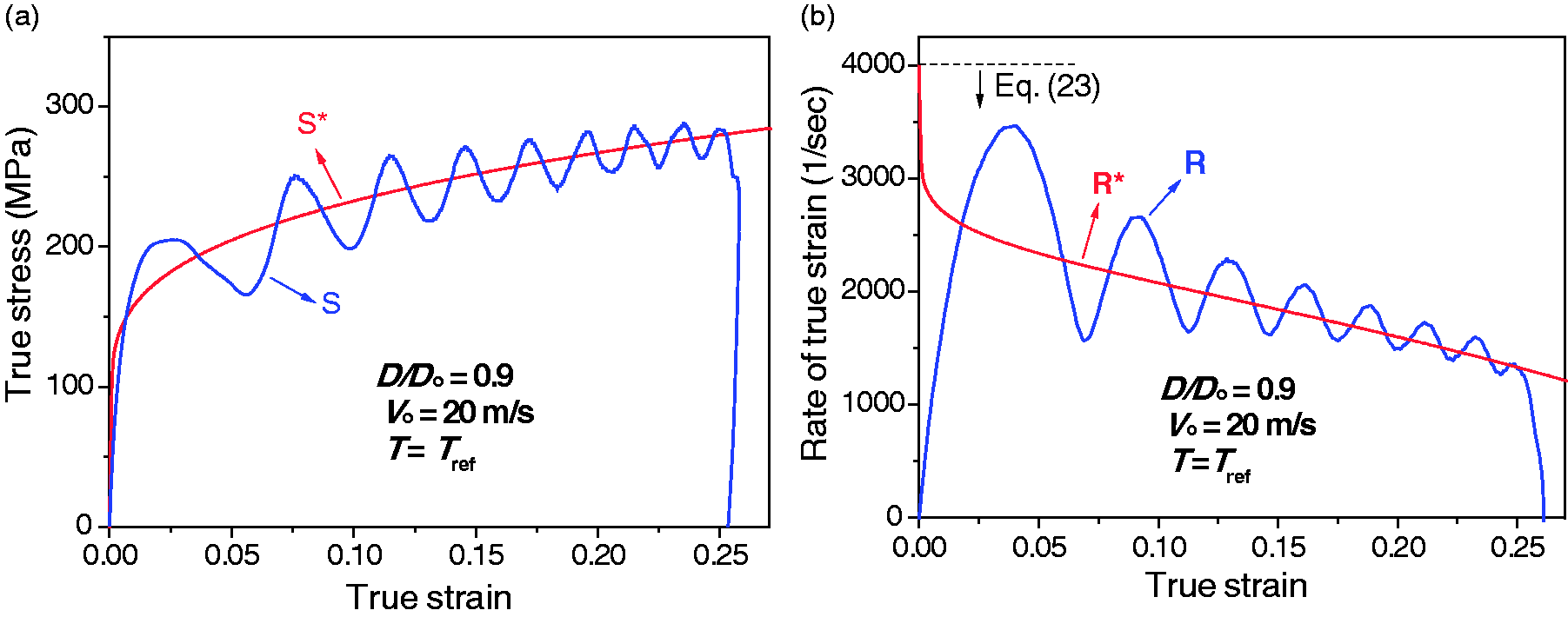

In a real experiment, the axial strain signals monitored in the bars ( $e_{R} (t)$ and $e_{T} (t)$ ) are used to measure the curves of stress–strain and rate–strain based on the SHB theory, e.g. equations (20) to (22). In the post-processing of the simulation result, the curves of stress–strain and rate–strain were also determined using the bar signals via equations (20) to (22). These curves constructed using the bar signals following the experimental procedure are named in this study as the ‘measured’ curves of stress–strain and rate–strain although the bar signals were obtained via the simulation.

The measured stress–strain curve using the bar signals in the simulation is presented in Figure 4(a) as curve S. Curve S fluctuates with strain; the reason for such fluctuation will be described later. In the real experiment, only the fluctuating curve S is measured. The two curves (S* and S) are consistent in that the measured curve S fluctuates around curve S* (the true material property defined prior to the numerical analysis). Indeed, the true material property (curve S*) manifests itself in the SHB test via the fluctuating curve S, which was measured using the bar signals. The consistency of the two curves (S* and S) numerically verifies the reliability of the SHB test: the SHB theory of measurement (equations (20)–(22)) and the instrument considered in this study (Tables 1 and 2) are reliable.

In Figure 4(b), curve R* was obtained by applying the defined stress–strain curve (S*) of the specimen into equation (10). According to the rate equation (equation (10)), curve R* is the rate of specimen that should be manifested (measured) in the SHB test if the specimen property is curve S*. Included in Figure 4(b) is curve R (the measured rate–strain curve using the bar signals), which is fluctuating with strain; the reason for such fluctuation is described in the next paragraph. In the real experiment, only the fluctuating curve R is measured. The two curves (R* and R) are consistent in that the measured curve R fluctuates around the predicted curve R* using the rate equation. Indeed, the predicted rate–strain curve using equation (10), i.e. curve R*, manifests itself in the SHB instrument via the fluctuating curve R, which was measured using the bar signals. The consistency of the two curves (R* and R) numerically verifies the formulated rate equation.

As already shown in Figure 4, the measured curves of S and R fluctuate significantly. Such fluctuation occurs because the bar signals ( $e_{R} (t)$ and $e_{T} (t)$ ) themselves oscillate with time, resulting in the fluctuation in the measured curves S and R using the bar signals. Such oscillation of the elastic wave in the bar results from inertia in the radial expansion of the bar⁶⁷ (the radial inertia effect is coupled with axial acceleration⁶⁸) and wave dispersion.^69,70 Such effects of inertia and wave dispersion inevitably appear in the elastic bar while such effects are not considered in the fundamental assumptions of the SHB; the same assumptions were employed in the derivation process of equation (10) (Assumptions section). Therefore, different from the measured curves S and R using the bar signals, there is no oscillation in curve R* predicted via the rate equation (equation (10)) from the non-oscillating curve S* (which is the true material property of the specimen defined prior to the numerical simulation).

Although remarkable consistency was observed between the curves R and R* in the plastic deformation regime (Figure 4(b)), there is a notable difference between the two curves in the small strain regime (up to the strain value of approximately 0.02 in the case of Figure 4(b)). In the fundamental (one-dimensional) theory of SHB,^24–35 a rectangle-shaped incident pulse (see Figures 1 –3) is assumed to be incident to the specimen owing to the assumption of no inertia: the slope of the stress–time (strain–time) curve in the rising part of the pulse is assumed to be infinite. It is further assumed that the stresses in the front and back surfaces of the specimen are the same (stress equilibrium; stress uniformity) even from the beginning of specimen deformation. Therefore, in the fundamental theory of the SHB, the characteristics of the specimen are assumed to manifest themselves from the beginning of specimen deformation in the SHB test. As the rate equation was derived under the same assumptions as the theory of the SHB, it also predicts that the rate of the specimen (curve R*) is manifested from the moment when the specimen deformation starts, i.e. when the specimen strain starts to increase from the value of zero. In Figure 4(b), the y-intercept value of curve R* constructed using the rate equation (equation (10)) is the predicted specimen strain rate when the specimen stress is zero at the strain value of zero (when the specimen starts to deform).

However, in reality, the slope of the rising part of the elastic pulse being incident to the specimen is finite because of the presence of (i) inertia. In particular, the front part of the stress pulse oscillates considerably because of inertia and (ii) wave dispersion. Furthermore, at the initial stage of specimen deformation, (iii) the uniformity of the specimen stress is not yet achieved. Owing to these three fundamental reasons (i)–(iii), it is well known^71–75 that the characteristics of the specimen in the SHB test cannot manifest themselves fully (properly) in the small strain regime, yielding the discrepancy between the fundamental theory of SHB and the measured curves (S and R). Because the specimen stain rate (curve R*) is not yet fully manifested in the SHB test at the initial stage of specimen deformation, there is a notable difference between the predicted curve R* using the rate equation (derived under the same assumptions as the fundamental theory of SHB) and the measured curve R in the SHB test in the small strain range.

In this section, the rate equation was verified numerically using the rate- and temperature-independent constitutive model (simulation case 1). The rate equation will also be verified both numerically (simulation case 2) and experimentally based on the correlation of the measured curves of stress–strain and rate–strain (Method for verifying the measured curves of rate–strain and stress–strain section). It will be verified numerically again in the Practical method of predicting the rate–strain curve section using the rate- and temperature-dependent constitutive model (simulation case 2).

Physical origin of the varying nature of strain rate in the SHB test

According to the formulated rate equation (equation (10)), the specimen strain rate is found out to be controlled by the stress and strain of the specimen during deformation, geometry (the length and diameter) of specimen, impedance of bar, and impact velocity. To reveal the varying nature (evolution) of the strain rate with strain (specimen deformation), the formulated rate equation (equation (10)) is analysed as follows.

The rate equation is composed of two terms. The first term in the right side of equation (10), i.e. V_o exp(ɛ)/L, increases the magnitude of the rate with strain (ɛ is positive). On the other hand, the second term, i.e. –2Aσ exp(2ɛ)/(A_oρ_oC_oL), decreases the magnitude of the rate with strain (σ is positive). Therefore, the specimen strain rate evolves as a result of the competition between the rate-increasing first term and rate-decreasing second term. Unless the first and second terms are balanced, the specimen strain rate generally varies (decreases or increases) with strain (with specimen deformation), which is the physical origin of the varying nature of the specimen strain rate in the SHB test.

The competition between the rate-increasing first term and the rate-decreasing second term is discussed here using the relative area (A/A_o) of the specimen and the stress of the specimen (σ), which appear only in the second term. When the rate-decreasing second term is more dominant (when the magnitudes of σ and A/A_o are considerably large), the strain rate decreases (with strain) in the plastic deformation regime, as can be observed in Figure 4(b) (and later in Figures 5(b) and 8(b)). When the rate-decreasing second term is negligible (when the magnitudes of σ and/or A/A_o are overly diminished) and thus the rate-increasing first term is dominant, the strain rate increases (with strain) in the plastic deformation regime. Such cases will be illustrated later in Figures 10 and 11.

In the literature, there has been no theory describing the varying nature of the specimen strain rate with deformation. Only the maximum limit of the specimen strain rate was described by the empirical relationship^33,34

\overset{\cdot}{ɛ} \leq V_{o} / L

(23)

The maximum rate limit predicted using equation (23) is indicated in Figure 4(b) by the dashed horizontal line. This line is drawn only up to a limited strain to avoid complexity. By purely judging from the result of Figure 4(b), where the strain rate decreases with strain because the rate-decreasing second term is dominant, equation (23) seems to predict the upper bound of the strain rate while equation (10) (curve R*) predicts a detailed change in the strain rate within the bound. However, when the rate-decreasing second term is diminished (when the magnitudes of σ and/or A/A_o are diminished), as will be illustrated later in Figures 10 and 11, equation (23) turns out to be invalid while equation (10) still predicts the strain rate reasonably even in such cases.

According to the second term of the rate equation, a higher strain rate is manifested in the SHB test if the flow stress of the specimen is low and vice versa for a high-stress (high-strength) specimen. This phenomenon is physically interpreted as follows. If a specimen exhibits a low stress, the input bar can push the specimen suitably (V₁ is high) while a low-stress (soft) specimen such as the foam material cannot push the output bar suitably (V₂ is low). According to Eqs. (1) and (2), such phenomena result in a higher magnitude of strain rate at a given impact velocity. If the specimen exhibits a high stress, the opposite result appears.

A final note on what the rate equation indicates is the influence of work hardening of the specimen on the strain rate. According to the second term of the rate equation (–2Aσ exp(2ɛ)/(A_oρ_oC_oL)), work hardening, i.e. the increase in specimen stress (σ) with strain (ɛ), augments the magnitude of the rate-decreasing second term with strain. Therefore, the phenomenon of work hardening certainly plays a role to decrease the slope of the rate–strain curve in the plastic deformation regime.

Method for verifying the measured curves of rate–strain and stress–strain

Correlation of measured curves of stress–strain and rate–strain

In the Numerical verification of rate equation section, the defined stress–strain curve of the specimen (curve S*) was converted via the rate equation to obtain the anticipated rate–strain curve in the SHB test (curve R*) for the purpose of verifying the formulated strain rate equation. It is evident that curve R* can also be converted back to curve S* via the strain rate equation. Therefore, the defined stress–strain curve of the specimen (curve S*) and the anticipated rate–strain curve in the SHB test (curve R*) are correlated with each other via the rate equation.

It is noted that the measured curves of stress–strain (S) and rate–strain (R) using the bar signals (equations (20) to (22)) can also be converted to each other via the rate equation. In this study, the converted rate–strain curve from the measured stress–strain curve (S) is named R**. According to the rate equation, if the experiment is to be valid (if the curves S and R were measured reliably in experiment), the curves R and R** should be coincident. The correlation of the measured curves of stress–strain (S) and rate–strain (R) can be checked from the coincidence of the curves R and R**.

Similarly, the converted stress–strain curve from the measured rate–strain curve (R) is named S** in this study. If the experiment is to be valid (if the curves S and R were measured reliably in experiment), the curves S and S** should be coincident. The correlation of the measured curves of stress–strain (S) and rate–strain (R) can also be checked from the coincidence of the curves S and S**.

In the next sections, whether or not the measured curve S is correlated with the measured curve R (i.e. whether or not the coincidence of curves S–S** as well as R–R** predicted by the rate equation is true) will be verified numerically first. Then, the correlation (coincidence) will be verified experimentally, followed by further discussions on the meaning and utilisation of the correlation (coincidence) phenomenon.

Numerical verification of correlation

The numerical simulation of the SHB test was carried out using the rate- and temperature-dependent constitutive model (case 2) of the specimen. The curves of stress–strain (S) and rate–strain (R) were constructed using the bar signals (equations (20) to (22)) and the results are shown in Figure 5.

Figure 5.

(a) Stress–strain curves and (b) rate–strain curves constructed using the bar signals obtained in numerical simulation case 2 that used the specimen with a rate- and temperature-dependent flow stress.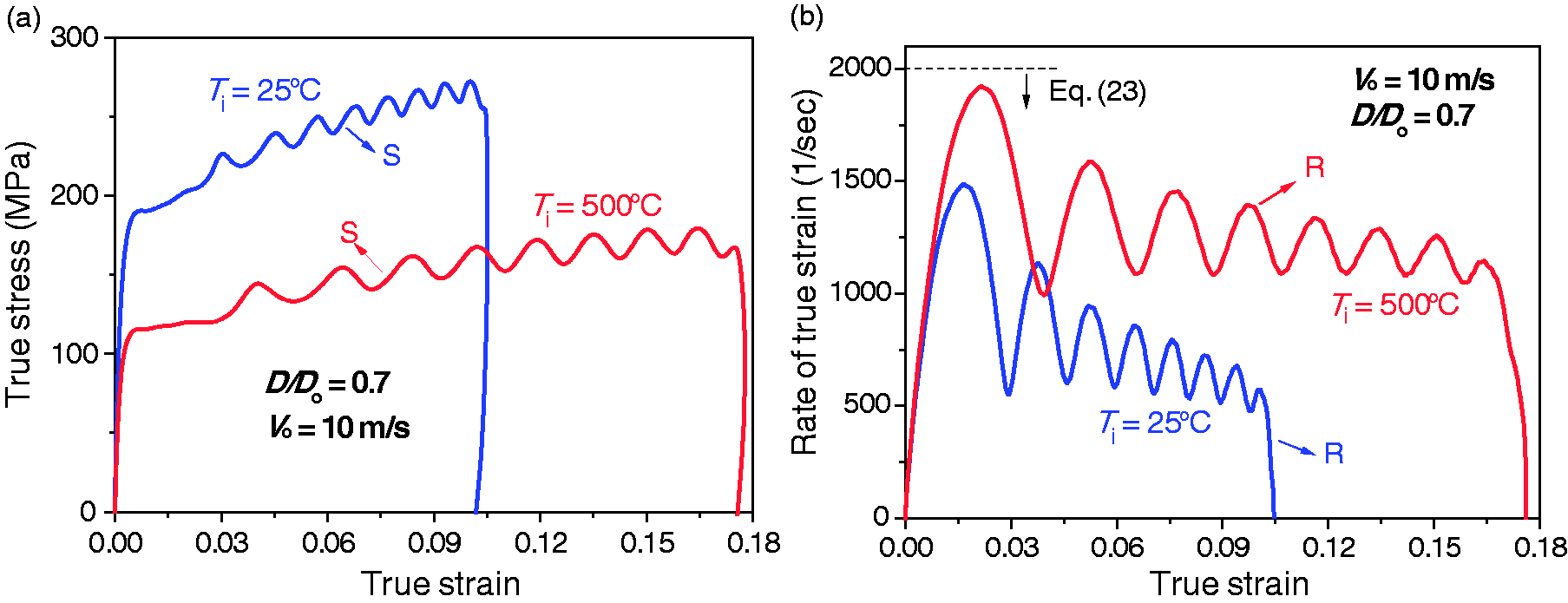

To verify whether the measured curves of S and R are correlated with each other, curve S in Figure 5(a) was applied into the rate equation. The converted curve is shown in Figure 6 as curve R**. Included in Figure 6 is the measured curve R. As can be observed in Figure 6, the fluctuating curves of R and R** coincide remarkably. Therefore, the measured rate–strain curve (R) is verified to be correlated with the measured stress–strain curve (S) via curve R**.

Figure 6.

Rate–strain curves obtained via numerical simulation (case 2) for cases where the initial temperatures of specimen were (a) 25 ℃ and (b) 500 ℃. The curve R in each figure was determined using the bar signals and curve R** was obtained by applying curve S (in Figure 5(a)) into equation (10).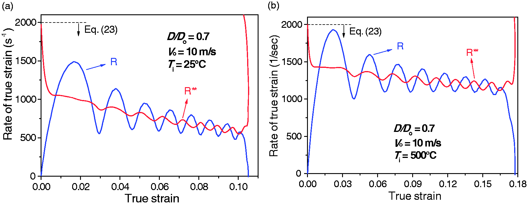

Curve R in Figure 5(b) was also applied into the rate equation. The converted curve is shown in Figure 7 as curve S**. Included in Figure 7 is the measured curve S. As can be observed in Figure 7, the fluctuating curves of S and S** coincide remarkably. Therefore, the measured stress–strain curve (S) is verified to be correlated with the measured rate–strain curve (R) via curve S**.

Figure 7.

Stress–strain curves obtained via numerical simulation (case 2) for cases where the initial temperatures of specimen were (a) 25 ℃ and (b) 500 ℃. The curve S in each figure was determined using the bar signals and curve S** was obtained by applying curve R (in Figure 5(b)) into equation (10).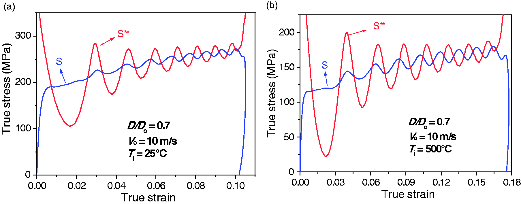

Experimental verification of correlation

The experimentally measured stress–strain curve of the OFC specimen with a D/D_o ratio of 0.7 is shown in Figure 8(a) as curve S. In Figure 8(b), curve R is the experimentally measured rate–strain curve. The measured curve S was applied into the rate equation and the converted rate–strain curve is presented as curve R**. A remarkable consistency of curves R and R** is observed, which experimentally verifies the correlation of the measured curves of S and R via curve R**.

Figure 8.

Experimentally obtained curves of (a) stress–strain and (b) rate–strain of an annealed OFC copper specimen. Curve S is the stress–strain curve obtained using the bar signals, and curve S** was determined by applying curve R into equation (10). Curve R is the rate–strain curve obtained using the bar signals, and curve R** was determined by applying curve S into equation (10).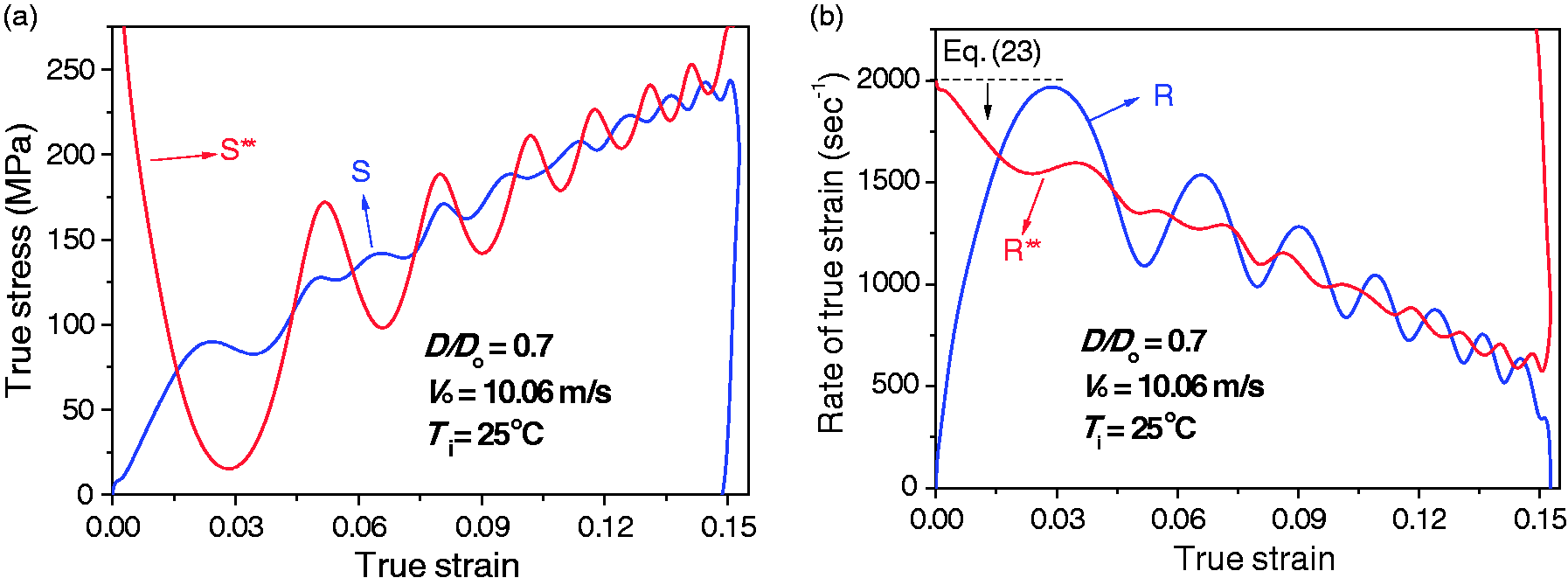

The experimentally measured curve R in Figure 8(b) was also applied into the rate equation and the converted stress–strain curve is presented as curve S** in Figure 8(a). Again, a remarkable consistency between curves S and S** is observed, which experimentally verifies the correlation of the measured curves of S and R via curve S**. The correlation of the experimentally measured curves of stress–strain and rate–strain for the specimens with D/D_o values of 0.4 and 0.2 is also presented later in Figure 11 and in the Supplemental Material available online.

Discussion on the correlation

As mentioned, the rate equation indicates that the measured curves of stress–strain (S) and rate–strain (R) are correlated. This point was verified both numerically and experimentally in the previous sections by demonstrating that the curves S and S** are coincident as well as the curves R and R**. Therefore, for the experiment and the bar-signal processing to be valid, the curves of S and R should reasonably coincide with S** and R**, respectively, as illustrated in Figures 6 to 8. In this regard, the rate equation can be used as a tool to verify the measured rate–strain curve simultaneously with the measured stress–strain curve, i.e. the reliability of the experiment. If the coincidence is not confirmed, it is necessary to check the experimental procedure or calibration of the SHB. The correlation method presented here can be used for the calibration of the SHB system as well.

As mentioned, the method that has been used in the literature to verify the measured stress–strain curve is comparing the stresses on the front and back surfaces of the specimen (stress equilibrium).^49–56 This method should be able to verify the measured stress–strain curve because the stresses on the specimen surfaces are checked; these stresses are measured from the signals of the input and output bars, respectively.^25–34 However, as mentioned, it is difficult to find a tool to verify the measured rate–strain curve in the literature. The correlation method using the rate equation here is independent of the stress-equilibrium method and checks the reliability of not only the measured stress–strain curve but also the measured rate–strain curve. Using the correlation method together with the stress-equilibrium method will enhance the verification tool, contributing to the maximal utilisation of the SHB.

In Figures 5(b) and 8(b), the measured curve R is highly fluctuating. Despite this highly fluctuating nature, it is certain that curve R in the considered cases decreases significantly in the plastic deformation regime. To clearly present the decreasing nature of the rate–strain curve in the plastic regime, a less-fluctuating rate–strain curve needs to be extracted from the highly-fluctuating curve R. However, in practice, it is generally difficult to reasonably extract a representative (less fluctuating) rate–strain curve solely by using curve R. In this regard, the intersection points between curves R and R** (Figures 6 and 8(b)) can be used to suitably extract a less-fluctuating rate–strain curve in the plastic regime. For instance, the intersection points in the plastic regime can be least-square fitted or nonlinearly curve-fitted to appropriate functions such as linear, hyperbolic, or polynomial functions; the type of the fitting function can be selected when the discrepancy between the considered fitting curve and the intersection points are minimal among the tested fitting functions. The representative rate–strain curve extracted in this way (the fitted curve to the intersection points in the plastic regime) can be used for the calibration of a rate-dependent constitutive model.

The intersection points between curves S and S** are not as useful as the intersection points between R and R** in the processing of the stress–strain curve (S) because curve S to be smoothed is generally less fluctuating compared with curve R. Nevertheless, the intersection points between curves S and S** can still be considered in the process of extracting a representative (less-fluctuating) stress–strain curve, which can be used for the calibration of the constitutive model.

What the rate equation (equation (10)) describes is the relationship between the stress–strain curve and rate–strain curve. Therefore, the numerical (simulation case 2) and experimental verifications of this relationship in the previous sections are indeed also the numerical and experimental verifications of the formulated rate equation itself.

Practical method of predicting the rate–strain curve

As mentioned, the state-of-the-art technology to obtain the target strain rate in the SHB test relies on trials or previous experience for specimens with similar property and geometry to those of the current specimen. In this section, it is numerically verified first whether predicting the rate–strain curve is possible using the rate equation and a given constitutive equation. Then, a discussion on the practical method to predict the rate–strain curve prior to the experiment follows.

Numerical verification of the method

The employed constitutive equation (equation (19)) describes the relationship between the stress (σ) and strain rate ( $\overset{\cdot}{ɛ}$ ) of the specimen at a given strain. Using solely equation (19), the stress (σ) of the specimen cannot be determined at a given strain unless the strain rate ( $\overset{\cdot}{ɛ}$ ) is known. However, note that the rate equation, equation (10), also describes the relationship between the stress (σ) and strain rate ( $\overset{\cdot}{ɛ}$ ) of the specimen at a given strain. Therefore, if equations (10) and (19) are solved simultaneously, the stress (σ) and strain rate ( $\overset{\cdot}{ɛ}$ ) of the specimen can be obtained simultaneously at a given strain.

In this study, equations (10) and (19) were solved numerically by employing the Newton–Raphson algorithm. The constitutive parameters listed in Table 3 were used for the JC model. In the process of solving the two equations, the temperature rise of the specimen was considered using information on the heat capacity and conversion percentage of plastic work to heat (inelastic heat fraction). The program to solve equations (10) and (19) is implemented in Excel® software. It can be downloaded in the Supplemental Material available online.

The stress–strain and rate–strain curves obtained using the above procedure are shown in Figure 9 as curves S* and R*, respectively. According to equations (10) and (19), curves S* and R* are the predicted stress–strain and rate–strain curves, respectively, which should be manifested (measured) in the SHB test if the instrument and the test theory (SHB theory) are correct.

Figure 9.

(a) Stress–strain curves and (b) rate–strain curves of simulation case 2.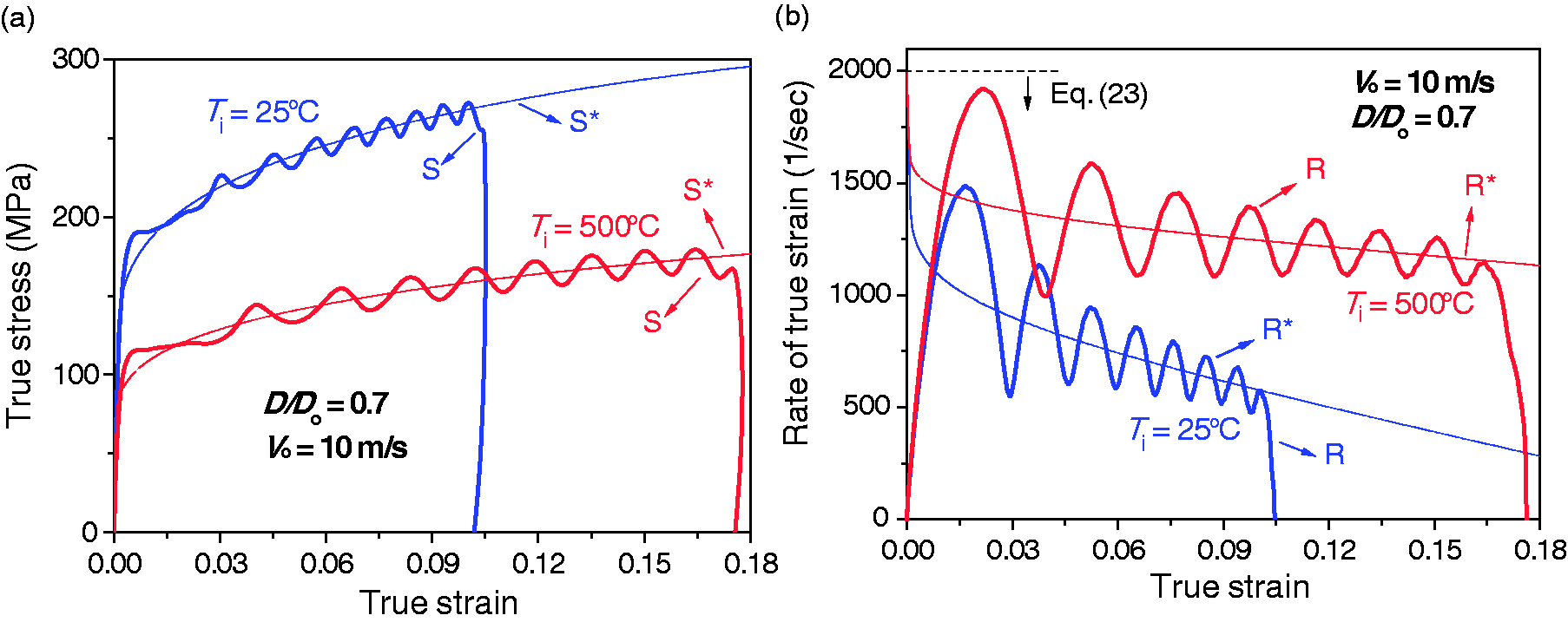

In Figure 9(a), curve S is the measured stress–strain curve using the bar signals in the simulation (case 2) of the SHB test. As can be observed in Figure 9(a), the measured curve S fluctuates around the predicted curve S* (the stress curve that should be measured in the SHB test); they are consistent. Indeed, the predicted stress curve (S*) manifests itself in the SHB instrument via the measured curve S. This finding indicates that the stress–strain curve (S*) can be predicted by simultaneously solving the rate and constitutive equations, and the predicted curve S* is reliable based on the measured curve S.

In Figure 9(b), curve R (the measured rate curve using the bar signals in the simulation) also fluctuates around curve R* (the predicted rate curve); they are consistent. Indeed, the predicted rate curve (R*) also manifests itself in the SHB instrument via the measured curve R. This finding indicates that the rate–strain curve (R*) can also be predicted by simultaneously solving the rate and constitutive equations, and the predicted curve R* is reliable based on the measured curve R.

In Figure 9, the reliability of the predicted curves S* and R* was verified by comparing the curves with the measured curves S and R, respectively. In other words, the measured curves S and R in the SHB test were used as the reference to verify the fact that the predicted curves S* and R* by simultaneously solving the rate and constitutive equations are reliable.

If the fact that the two equations (equations (10) and (19)) with two unknown variables (σ and $\overset{\cdot}{ɛ}$ ) at a given strain can be solved simultaneously is admitted, the fact that exactly what the rate equation predicts (S* and R*) are measured (manifested) via curves S and R in the SHB test verifies again the rate equation itself via the numerical simulation (case 2).

Practical method of predicting the rate–strain curve

It was demonstrated in the previous section that the curves of rate–strain and stress–strain, which should be measured (manifested) in the SHB test, can be predicted before carrying out the SHB test using the rate equation provided the constitutive parameters are available. In reality, the constitutive parameters are unknown for the specimen to be tested using the SHB. However, the constitutive parameters of the specimen can be reasonably estimated as follows.

In general, the quasi-static test of a specimen is carried out before the SHB test. If two or more stress–strain curves are measured at two or more different strain rates in the quasi-static test (e.g. 10⁻⁵ and 10⁻² s⁻¹), the values of a, b, n, and c in equation (19) can be determined suitably via non-linear curve fitting of the measured stress–strain curves. As for the thermal softening parameter (m), it is noted that its value does not vary significantly for similar types of material.⁸ For instance, the values of m for 1006 steel, 4340 steel, and S-7 tool steel are 1.00, 1.03, and 1.00, respectively. The values for aluminium alloy 2024-T351 and aluminium alloy 7039 are 1.00 and 1.00, respectively. The values for Armco® iron and Carpenter® electrical iron are 0.55 and 0.55, respectively. Therefore, the value of m for similar types of material to the current specimen can be reasonably obtained from the literature. Within the framework of equation (19), there is no error in the method itself for calibrating the parameters, a, b, n, and c. On the other hand, the error in the selected value of m from the literature is inevitable and unquantifiable. However, as mentioned, the selected value of m in this way should not be far away from that of the current specimen.

The above paragraph described the procedure for reasonably estimating the parameters of the JC model⁸ employed in this study. This model probably has been used and calibrated most extensively for simulating many high-strain-rate events of materials and structures. However, there are indeed numerous types of constitutive models, which were developed for capturing various aspects of complicated constitutive behaviours of versatile materials. For instance, when the specimen material exhibits the phenomenon of stress upturn and the material is to be tested in the strain rate regime where the stress upturn takes place, the use and calibration of a stress upturn model⁹ would be more desirable than the JC model. When the phenomena of rate-hardening and temperature-softening are coupled¹⁰ or when strain-hardening and rate-hardening are coupled,¹¹ models developed for such cases^10,11 would be more appropriate. A similar procedure to the JC model described in the above paragraph can be employed for the reasonable estimation of the parameters of such other constitutive models.

Once the constitutive parameters are reasonably estimated as above, the curves of rate–strain and stress–strain which are anticipated to be manifested (measured) in the SHB test can be predicted simultaneously using the Excel® program provided in the Supplemental Material. While this study illustrates the usage of the rate equation by combining it with the JC model, the provided program can be modified suitably for different constitutive models.

As mentioned, according to equation (10), the specimen strain rate is controlled by the stress of the deforming specimen, geometry (the length and diameter) of specimen, impedance of bar, and impact velocity. One can suitably explore the effects of these variables by inputting appropriate values in the spread sheet cells in the provided Excel® file, and the resulting curves of rate–strain and stress–strain are updated immediately after running the program. For the design of experiment, prediction of the rate–strain curve in this way before carrying out the SHB test should be more desirable than determining the manifested rate–strain curve after the experiment is finished.

Predicting the maximum strain

Neither the rate equation nor constitutive equation has a limit in strain (there is no strain limit in drawing curves S* and R*) as far as the strain rate is positive. The specimen strain measured in the SHB test can be limited by the pulse duration time and fracture of the specimen. This study considers the case where the specimen strain is limited by the pulse duration time $(t_{p} = 2 L_{o} / C_{o})$ ; it is assumed that specimen fracture does not occur meanwhile the stress pulse passes the specimen. The maximum specimen strain ( $ɛ_{max}$ ) in the SHB test is determined by the pulse duration (passage) time (t_p) and the specimen strain rate: $ɛ_{max} = t_{p} \overset{\cdot}{ɛ}$ . Because the pulse duration time is fixed in an SHB test, a higher rate of the specimen results in a higher maximum strain.

In the current technology, the maximum strain that a specimen experiences in the SHB test is revealed only after the test is finished. However, once the rate–strain curve is available prior to the SHB test, the maximum strain can be predicted by combining the rate–strain curve with the pulse duration time. The method calculates the incremental deformation time (dt) at each strain step (dɛ): $dt = \frac{d ɛ}{\overset{\cdot}{ɛ}}$ . Then, the value of the strain at the moment when the cumulative deformation for each strain step reaches the pulse duration time (t_p) is determined to be the maximum strain. The algorithm to predict the maximum strain in this way is included in the Excel® program. It considers the condition that the strain rate should be positive. The predicted maximum strains using the Excel® program are reasonably consistent with the results of the numerical simulation in Figure 4 (0.265) and Figure 5(b) (0.109 and 0.181). It is also the case in Figure 10(b) (0.234) and Figure 10(c) (0.320), which will be presented later.

Figure 10.

(a) Rate–strain curves (R*) predicted using the rate equation for a range of D/D_o values. Simulated curves of R superimposed to curves R* when D/D_o values are (b) 0.41 and (c) 0.15 (simulation case 2).

Figure 11.

Experimentally determined rate–strain curves of annealed OFC specimens with a range of relative diameters (D/D_o). The curves for D/D_o = 0.7 are the same as in Figure 8(b). The predicted bound for each specimen using equation (23) is the y-intercept of curve R**, which is not marked additionally to avoid complexity.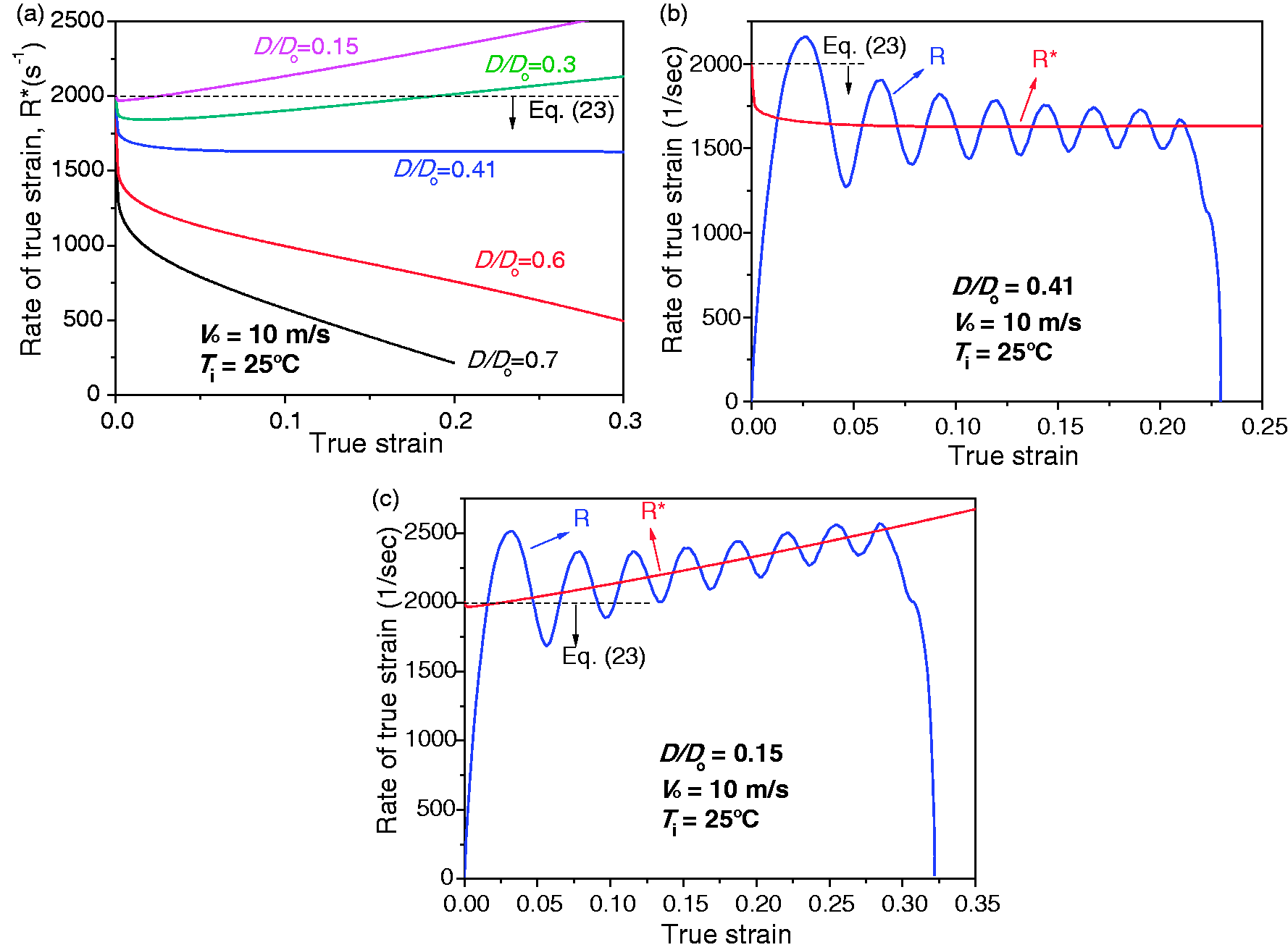

Tailoring the slope of the rate–strain curve by controlling the specimen diameter

From the analysis on the two terms of equation (10) in the Physical origin of the varying nature of strain rate in the SHB test section, it is postulated that if the rate-increasing first term, V_o exp(ɛ)/L, and rate-decreasing second term, −2Aσ exp(2ɛ)/(A_oρ_oC_oL), are brought into competition, the decreasing/increasing nature of the rate–strain curve, i.e. the slope of the rate–strain curve in the plastic deformation regime, can be tailored. Among the parameters in the first and second terms, controlling the magnitude of A/A_o appearing only in the second term may be most suitable for the competition of the two terms. The D/D_o ratio is used hereafter instead of the A/A_o ratio for convenience.

In the next sections, it is first verified numerically whether or not tailoring the slope of the rate–strain curve is possible by controlling the specimen diameter, followed by experimental verification. A discussion on the practical methods to determine the D/D_o ratio for achieving a nearly constant strain rate finally follows.

Numerical verification of the approach

To monitor the result of competition of the two terms by controlling the D/D_o ratio, the rate–strain curves (R*) were predicted by solving equations (10) and (19) simultaneously using the Excel® program (Supplemental Material) for a range of D/D_o ratios; the result is shown in Figure 10(a). As can be observed in Figure 10(a), if the D/D_o value decreases from 0.7 to 0.41, the slope of the rate–strain curve in the plastic regime increases towards a positive value and a nearly constant strain rate is achieved at the D/D_o value of 0.41 (this value is limited to the employed properties of the specimen and bar (Tables 2 and 3) at the given impact condition). To check whether the nearly constant rate is really manifested in the SHB test when the D/D_o value is 0.41, a numerical simulation (case 2) of the SHB test was carried out. The rate–strain curve measured using the bar signals is illustrated in Figure 10(b) as curve R. Indeed, the nearly constant strain rate (curve R* predicted using the rate equation) manifests itself via the measured curve R using the bar signals; they are reasonably coincident. Comparing with the case where D/D_o = 0.7 (Figure 9(b) at T_i = 25 ℃), the result for D/D_o = 0.41 in Figure 10(b) is a notable improvement in achieving a nearly constant strain rate during dynamic deformation of a work-hardening specimen.

In Figure 10(a), if the D/D_o value decreases further from 0.41 to 0.30, interestingly, the slope of the rate–strain curve now becomes positive and the slope increases further with a further decrease in the D/D_o value to 0.15. Another important point for the specimen with the D/D_o value of 0.15 is that the magnitude of the strain rate itself is higher than the maximum limit predicted using equation (23), indicating the invalidity of equation (23). These observations result from the fact that the influence of the rate-decreasing second term of equation (10), –2Aσ exp(2ɛ)/(A_oρ_oC_oL), is overly diminished at small values of D/D_o compared with the influence of the rate-increasing first term, V_o exp(ɛ)/L. To check whether the predicted R* curve with such characteristics is really manifested in the SHB experiment when the D/D_o value is 0.15, a numerical simulation (case 2) of the SHB test was carried out. The rate–strain curve measured using the bar signals is shown in Figure 10(c) as curve R. Indeed, the coincidence between the measured curve R and predicted curve R* (using the rate equation) is confirmed; the predicted curve R* using the rate equation manifests itself in the SHB test via the measured curve R. Therefore, when the D/D_o value is exceedingly small (when the rate decreasing second term is overly diminished), it is natural to observe (i) the positive slope of the rate–strain curve in the plastic deformation regime, and (ii) the magnitude of the strain rate can be higher than the maximum limit predicted using equation (23).

Overall, the results in Figure 10 numerically verify that the slope of the rate–strain curve in the plastic deformation regime can be tailored by controlling the specimen diameter. The slope can be controlled to be either negative or positive.

Experimental verification of the approach

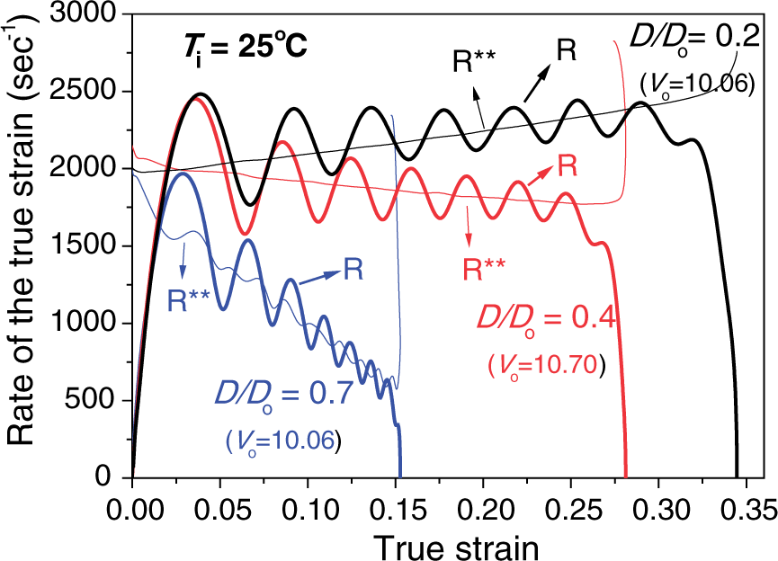
A series of SHB experiments was carried out using annealed OFC specimens with a range of relative diameters. The experimentally measured rate–strain curves are shown in Figure 11 as curve R at each impact condition. Included in Figure 11 is curve R**, which was obtained by applying the experimentally obtained stress–strain curve (S) presented in the Supplemental Material into the rate equation. In Figure 11, depending on the D/D_o value, the change in the slope of the strain rate in the plastic deformation regime is apparent. The result in Figure 11 experimentally verifies that the slope of the rate–strain curve can be modified suitably by controlling the specimen diameter.

In Figure 11, curves R and R** are reasonably coincident for all the considered specimen diameters in the experiment. In the Supplemental Material, curves S and S** are also reasonably coincident for all the considered specimen diameters. These findings experimentally verify the rate equation again.

Practical methods of determining the specimen diameter for achieving a nearly constant strain rate

For the case of D/D_o = 0.7 in Figure 11, the specimen strain rate in the plastic deformation regime (the intersection points between curves R and R**) varies from approximately 1700 to 615 s⁻¹. If the rate dependency of the specimen is not high (i.e. if the stresses measured at the strain rates of 1700 and 615 s⁻¹ are not much different), the necessity of finding the optimum D/D_o value for achieving a constant strain rate may not be high. If the specimen exhibits a high rate dependency, it may be necessary to test the material properties at a constant strain rate.

The analytical expression of the D/D_o value for achieving a constant specimen strain rate, (D/D_o)_c, can be obtained by differentiating equation (10) with respect to ɛ, i.e. from the condition of 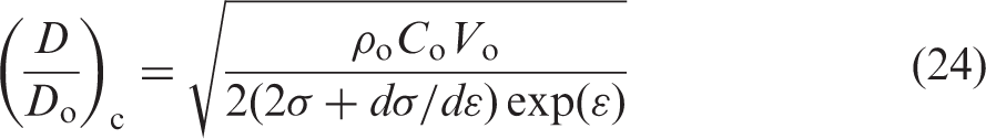$d \overset{\cdot}{ɛ} / d ɛ = 0$ :

\begin{matrix} (\frac{D}{D_{o}})_{c} = \sqrt{\frac{ρ_{o} C_{o} V_{o}}{2 (2 σ + d σ / d ɛ) exp (ɛ)}} \end{matrix}

(24)

In equation (24), the governing parameters of (D/D_o)_c include not only specimen-independent parameters (impact velocity and impedance of the bar) but also specimen-dependent parameters (strain ( $ɛ$ ), stress (σ), and strain derivative of stress ( $d σ / d ɛ$ )). Because the specimen parameters vary with strain, there is no single (D/D_o)_c value for the perfectly constant strain rate as the strain increases; the (D/D_o)_c value varies with strain. This is the theoretical reason that only a nearly constant strain rate is achieved in the SHB test even when the D/D_o value is appropriately tuned, as can be observed in curve R* in Figure 10(b).

It is noted in equation (24) that, if a given stress–strain curve is applied into the equation, a (D/D_o)_c versus strain plot is obtained. It is aimed here to check whether the plot of (D/D_o)_c versus strain obtained in this way is useful for determining the optimum value of D/D_o to achieve a nearly constant strain rate. If (i) a dynamic stress–strain curve to be applied into equation (24) is available and, at the same time, (ii) the correct answer of the optimal D/D_o value for the dynamic stress–strain curve is known in advance, it is possible to check whether the (D/D_o)_c versus strain plot is useful to determine the optimum D/D_o value. In this study, the necessary dynamic stress–strain curve as well as the correct value of the optimum D/D_o was obtained by solving equation (10) and equation (19) for a range of D/D_o values at three impact velocities (10, 20, and 30 m/s) using the Excel® program. As the result, the nearly constant strain rates were achieved at D/D_o values of 0.34, 0.48, and 0.58 at impact velocities of 10, 20, and 30 m/s, respectively, for the SHB instrument (Tables 1 and 2) and a 5 mm-thick Armco® iron specimen (a = 175 MPa, b = 380 MPa, n = 0.32, c = 0.06, m = 0.55, T_m = 1811 K, T_ref = 298 K, ${\overset{\cdot}{ɛ}}_{o}$ = 1 s⁻¹, E = 207 GPa, ρ = 7890 kg/m³, and c_p = 452 Jkg^-1K^-1).^8,a The obtained stress–strain curves and rate–strain curves for the iron specimen are shown in Figure 12(a) and Figure 12(b), respectively. From these figures, it is clear that the D/D_o values of 0.34, 0.48, and 0.58 are the correct values (answers) for achieving a nearly constant rate at respective impact velocities. It is aimed here to verify whether the plot of (D/D_o)_c versus strain obtained by applying the stress–strain curves of Figure 12(a) into equation (24) can help one in finding the answers.

Figure 12.

(a) Stress–strain curves and (b) rate–strain curves at (D/D_o)_c values of 0.34, 0.48, and 0.58 and impact velocities of 10, 20, and 30 m/s, respectively. The considered specimen material was Armco® iron at the initial temperature of 298 K. They were obtained by solving equation (10) and equation (19). (c) (D/D_o)_c curves obtained by applying the three stress–strain curves in (a) into equation (24). The quasi-static stress–strain curve in (a) was constructed under the isothermal assumption at 298 K.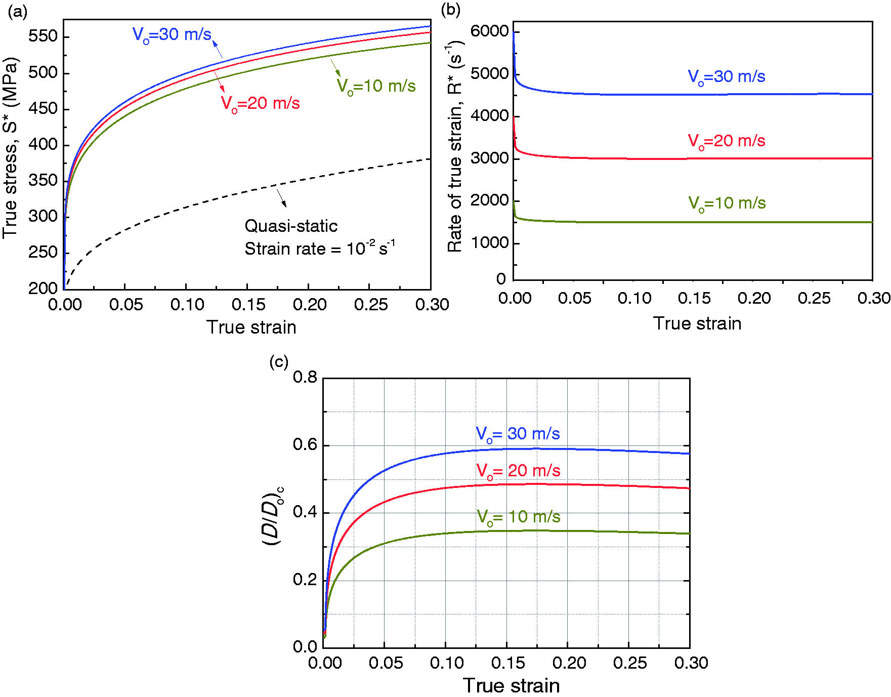

Figure 12(c) shows the plots of (D/D_o)_c versus strain, which were obtained by applying the three dynamic stress–strain curves of Figure 12(a) into equation (24). As can be observed in Figure 12(c), the (D/D_o)_c curves vary significantly with strain especially when the value of the strain is less than approximately 0.1. Revisiting equation (24) and Figure 12(a), the change in σ and $d σ / d ɛ$ with strain is significant when the value of the strain is less than approximately 0.1, which explains the reason that the (D/D_o)_c curves in Figure 12(c) vary significantly with strain in the mentioned strain regime.

However, the (D/D_o)_c curves in Figure 12(c) do not vary very significantly thereafter (when the value of the strain is larger than approximately 0.1) because the change in σ and $d σ / d ɛ$ with strain is insignificant as can be observed in Figure 12(a). One may select the average value in the strain range of approximately between 0.1 and 0.3 where the (D/D_o)_c curve does not vary greatly. Then, the optimal D/D_o value determined using the (D/D_o)_c curves in Figure 12(c) should not deviate considerably from the answers, i.e. the optimum D/D_o values of 0.34, 0.48, and 0.58, respectively. Therefore, it is concluded that the (D/D_o)_c versus strain plot constructed by applying an appropriate stress–strain curve into equation (24) is useful to determine the optimum D/D_o value for achieving a nearly constant strain rate.

In the above paragraphs, the usefulness of the (D/D_o)_c versus strain plot in determining the optimum value of D/D_o was numerically verified. For the verification purpose, stress–strain curves (Figure 12(a)) determined from the known constitutive parameters and the known answers of the (D/D_o)_c values (Figure 12(b)) for the considered stress–strain curves were used. In reality, however, the dynamic stress–strain curve to be applied into equation (24) is unavailable before carrying out the SHB test. Therefore, in essence, the optimum D/D_o value for achieving a nearly constant strain rate has to be determined experimentally by trials. However, the first trial value of D/D_o can be reasonably estimated as described in the following paragraphs.

To determine the first trial value of D/D_o for achieving a nearly constant rate–strain curve, this study presents two practical methods as follows. The first practical method to determine the first trial value of D/D_o is using equation (24). The input stress–strain curve to equation (24) can be obtained by multiplying the rate factor (the second bracket in equation (19)) and temperature factor (the third bracket in equation (19)) to a stress–strain curve measured at a quasi-static strain rate and temperature, which is considered as the reference curve (measured at ${\overset{\cdot}{ɛ}}_{o}$ and $T_{ref}$ ). The methods of obtaining the parameters c and m in the rate and temperature factors, respectively, were previously described in the Practical method of predicting the rate–strain curve section. The resultant (D/D_o)_c vs. strain plot constructed by applying the input stress–strain curve into equation (24) can be used to determine the first trial value of D/D_o.

The second practical method to find the first trial value of D/D_o is using the rate equation itself, equation (10), instead of using its strain derivative, i.e. equation (24). As described in the Practical method of predicting the rate–strain curve section, the constitutive parameters can be reasonably estimated from a couple of quasi-static tests and by referring to the value of m in the literature for similar types of materials. Then, the numerical solution for equation (10) and equation (19) (using the provided Excel® program) will readily produce the rate–strain curves such as the ones shown in Figure 10(a) for a range of D/D_o values, which will allow one to determine the D/D_o value for the first trial to obtain a nearly constant strain rate. Actually, constructing the anticipated rate–strain curve in this way is desirable before carrying out the SHB test.

In the SHB test, the use of the specimen with the first trial value of D/D_o based on either of the methods presented above should be more appropriate than using the specimen with an arbitrary D/D_o value because the latter may yield a significantly varying strain rate of the deforming specimen (such as curve R in Figure 8 when the D/D_o value is 0.7). Even the first trial value of D/D_o determined by the presented methods may not be far away from the optimum value: the manifested (measured) rate–strain curve in the SHB test using the first trial D/D_o value would be much closer to a nearly constant state compared with the case of using an arbitrary diameter. The D/D_o value can be tuned further via the second-trial test only when a better nearly-constant strain rate than the first-trial test result is necessary. As can be observed in Figure 10(a), if the slope of the rate–strain curve in the plastic deformation regime needs to be increased, a smaller D/D_o value (which reduces the magnitude of the rate-decreasing second term of the rate equation) is required for the second trial and vice versa to decrease the slope of the rate–strain curve in the plastic regime.

The rate equation not only provides a theory-based handy method for achieving a nearly constant strain rate by controlling the specimen diameter but also drastically speeds up the convergence process towards the optimum D/D_o value by providing the first trial value, which is anticipated to be reasonably close to the optimum value. Even when the second or more trial tests are needed, the systematic progress of convergence to the optimum D/D_o value can be suitably monitored because the process of determining the optimum D/D_o value after the first trial test (described in the above paragraph) is a closed loop process that utilises the feedback of the previous test result. Being able to monitor such a systematic convergence is a big advantage of the closed loop control process.

Overall discussion: The rate equation within the boundary of SHB theory

This study formulated the strain rate equation (equation (10)), and presented some application areas. As the same assumptions as the fundamental theory of SHB (Assumptions section) were employed in the derivation process of the rate equation, the rate equation does not contradict the SHB theory but is within its boundary. The rate equation allows one to investigate an unexplored area in the classic (one-dimensional) SHB theory: the evolution of the specimen strain rate with strain (specimen deformation).

Conclusion

To reveal the physical origin of the varying nature of specimen strain rate during deformation in the SHB test, the strain rate has been formulated as a function of strain (specimen deformation) based on a one-dimensional assumption. According to the formulated rate equation (equation (10)), the specimen strain rate is governed by the stress and strain of specimen during deformation, geometry (the length and diameter) of specimen, impedance of bar, and impact velocity. The rate equation is composed of two terms: the rate-increasing first term (V_o exp(ɛ)/L) and the rate-decreasing second term (−2Aσ exp(2ɛ)/(A_oρ_oC_oL)). Therefore, the specimen strain rate evolves as a result of the competition between the rate-increasing first term and rate-decreasing second term. Unless these two terms are balanced, the specimen strain rate generally varies (decreases or increases) with strain (specimen deformation), which is the physical origin of the varying nature of the specimen strain rate in the SHB test. The increase in specimen stress during deformation (e.g. work hardening), appearing in the second term, plays a role in decreasing the slope of the rate–strain curve in the plastic deformation regime.

According to the formulated strain rate equation, the measured curves of stress–strain and rate–strain are mutually correlated. The rate equation can be used as a tool to verify the measured rate–strain curve simultaneously with the measured stress–strain curve, i.e. to verify the reliability of the experiment. If the experimentally measured curves of stress–strain (S) and rate–strain (R) are superposed to the curves of S** and R**, which were converted from curves of R and S, respectively, using the rate equation, the curves of S and S** should be coincident as well as the curves of R and R**. Otherwise, it is be necessary to check the experimental procedure and instrument calibration. The method of correlation can also be used as a tool for the calibration of the instrument. The intersection points between curves R and R** (S and S**) can be used to extract a less-fluctuating rate–strain (stress–strain) curve, which can be used as representative curves of stress–strain and rate–strain for the calibration of a rate-dependent constitutive model.

It has been numerically demonstrated that the rate–strain curve and stress–strain curve measured in the SHB test can be predicted before carrying out the test by simultaneously solving the rate equation and a constitutive equation. The program for solving the two equations is implemented in the Excel® software, which is available in the Supplemental Material. For practical prediction of the curves of the rate–strain and stress–strain, the constitutive parameters of the Johnson–Cook (JC) model can be reasonably estimated from a couple of quasi-static tests together with referring to the thermal softening parameter of a similar type of material to the current specimen in the literature. The parameters of other constitutive models can also be reasonably estimated similarly.

Once the rate–strain curve is available, the maximum specimen strain in the SHB test can be predicted by combining the rate–strain curve with the pulse duration time. Such an algorithm is also included in the Excel® program.

It has also been demonstrated both numerically and experimentally that the slope of the rate–strain curve in the plastic deformation regime can be tailored by controlling the diameter of the specimen. Two practical methods to determine the value of the relative diameter (D/D_o) for achieving a nearly constant strain rate are presented. The first method is using the (D/D_o)_c vs. strain plot which can be constructed by applying an input stress–strain curve into equation (24); the input curve can be obtained by multiplying the rate and temperature factors of the JC model to a quasi-static stress–strain curve. The second method is simultaneously solving the rate equation and a reasonably estimated constitutive equation (using the Excel® program) for a range of D/D_o values.

As the same assumptions as the fundamental theory of SHB were employed in the derivation process of the rate equation, the rate equation is within the boundary of the SHB theory. The rate equation allows one to investigate an unexplored area in the classic (one-dimensional) SHB theory: the evolution of the specimen strain rate with strain (specimen deformation).

Supplemental Material 1

Supplemental Material1 - Supplemental material for Evolution of specimen strain rate in split Hopkinson bar test

Supplemental material, Supplemental Material1 for Evolution of specimen strain rate in split Hopkinson bar test by Hyunho Shin and Jong-Bong Kim in Proceedings of the Institution of Mechanical Engineers, Part C: Journal of Mechanical Engineering Science

Supplemental Material 2

Supplemental Material2 - Supplemental material for Evolution of specimen strain rate in split Hopkinson bar test

Supplemental material, Supplemental Material2 for Evolution of specimen strain rate in split Hopkinson bar test by Hyunho Shin and Jong-Bong Kim in Proceedings of the Institution of Mechanical Engineers, Part C: Journal of Mechanical Engineering Science

Footnotes

Declaration of Conflicting Interests

The author(s) declared no potential conflicts of interest with respect to the research, authorship, and/or publication of this article.

Funding

The author(s) disclosed receipt of the following financial support for the research, authorship, and/or publication of this article: This study was financially supported by the Basic Science Research Program under contract number 2015R1A2A2A01002454 (HS) through a National Research Foundation of Korea (NRF-Korea) grant.

Supplemental material

Supplemental material for this article is available online.

Note

References

Olcmen

Jones

Weiner

. A numerical analysis of projectile nose geometry including sliding friction for penetration into geological targets. Proc IMechE, Part C: J Mechanical Engineering Science 2016; 232: 284–304.

Heimbs

Ritzer

Markmiller

. Numerical method for blast shock wave analysis of missile launch from aircraft. Int J Aerospace Eng 2015; 2015: 897213 ,

Breslavsky

Morachkovsky

Naumov

et al.

Deformation and fracture of square plates under repetitive impact loading. Int J Non-Linear Mech 2018; 98: 180–188.

Chen

Ren

Yang

Guo

. Evidence of thermoplastic instability about segmented chip formation process for Ti-6Al-4V alloy based on the finite-element method. Proc IMechE, Part C: J Mechanical Engineering Science 2011; 225: 1407–1417.

Yoo

Y-H

Baek

Kim

J-B

et al.

Performance of a flying cross bar to incapacitate a long-rod penetrator based on a finite element model. Eng Computers 2013; 29: 409–415.

Altenbach H, Breslavsky D, Naumenko K, et al. Two-time-scales and time-averaging approaches for the analysis of cyclic creep based on Armstrong-Frederick type constitutive model. Proc IMechE, Part C: J Mechanical Engineering Science 2018, http://journals.sagepub.com/doi/10.1177/0954406218772609#.

Cho

Kaneko

. Influence of the applied pressure waveform on the dynamic fracture processes in rock. Int J Rock Mech Mining Sci 2004; 41: 771–784.

Johnson GR and Cook WH. A constitutive model and data for metals subjected to large strains, high strain rates and high temperatures. In: Proceedings of the 7th international symposium on ballistics, The Hague, Netherlands, 19–21 April 1983, pp.541–547.

Shin

Kim

J-B

. A phenomenological constitutive equation to describe various flow stress behaviors of materials in wide strain rate and temperature regimes. J Eng Mater Technol 2010; 132: 021009.

10.

Zerilli

Armstrong

. Dislocation-mechanics based constitutive relations for material dynamics calculations. J Appl Phys 1987; 61: 1816–1825.

11.

Khan

Kazmi

Farrokh

. Multiaxial and non-proportional loading responses, anisotropy and modeling of Ti–6Al–4V titanium alloy over wide ranges of strain rates and temperatures. Int J Plasticity 2007; 23: 931–950.

12.

Fardmoshiri

. Constitutive model calibration at high strain rate using Hopkinson bar, Sarrbrücken: Scholars' Press, 2016.

13.

L-Y

Molyneaux

TCK

. Dynamic constitutive equations and behaviour of brass at high strain rates. Proc IMechE, Part C: J Mechanical Engineering Science 1995; 209: 287–293.

14.

Piao

Huh

Lee

Park

. Characterization of hardening behaviors of 4130 Steel, OFHC Copper, Ti6Al4V alloy considering ultra-high strain rates and high temperatures. Int J Mech Sci 2017; 131–132: 1117–1129.

15.

Lee

W-S

Chen

T-H

. Plastic deformation and fracture characteristics of Hadfield steel subjected to high-velocity impact loading. Proc IMechE, Part C: J Mechanical Engineering Science 2002; 216: 971–982.

16.

Khan

Liu

Yoon

Nambori

. Strain rate effect of high purity aluminum single crystals: experiments and simulations. Int J Plasticity 2015; 67: 39–52.

17.

Wang

. Cutting forces model for milling Inconel 718 alloy based on a material constitutive law. Proc IMechE, Part C: J Mechanical Engineering Science 2012; 227: 1761–1775.

18.

Seo

Min

Yang

. Constitutive equation for Ti–6Al–4V at high temperatures measured using the SHPB technique. Int J Impact Eng 2005; 31: 735–754.

19.

Chen

Wang

. Analytical modelling of cutting forces in near-orthogonal cutting of titanium alloy Ti6Al4V. Proc IMechE, Part C: J Mechanical Engineering Science 2015; 229: 1122–1133.

20.

Sedighi

Khandaei

Shokrollahi

. Identification of optimized constitutive model parameters at a high strain rate using electromagnetic ring expansion test results. Proc IMechE, Part C: J Mechanical Engineering Science 2011; 225: 781–789.

21.

Park

Moon

Bae

et al.

Strain rate effects of dynamic compressive deformation on mechanical properties and microstructure of CoCrFeMnNi high-entropy alloy. Mater Sci Eng: A 2018; 719: 155–163.

22.

Lee

W-S

Lin

C-F

Huang

S-Z

. Effect of temperature and strain rate on the shear properties of Ti-6Al-4V alloy. Proc IMechE, Part C: J Mechanical Engineering Science 2006; 220: 127–136.

23.

Salehghaffari

Rais-Rohani

. Material model uncertainty quantification using evidence theory. Proc IMechE, Part C: J Mechanical Engineering Science 2013; 227: 2165–2181.

24.

Hopkinson

. A method of measuring the pressure produced in the detonation of high explosives or by the impact of bullets. Philos Trans R Soc Lond Series A 1914; 213: 437–456.

25.

Kolsky

. An investigation of the mechanical properties of materials at very high rates of loading. Proc Phys Soc Lond Sect B 1949; 62: 676–700.

26.

Wang L-l. Foundations of stress waves. London: Elsevier, 2007.

27.

Meyers

. Dynamic behavior of materials, New York, NY: John Wiley & Sons, Inc., 1994.

28.

Chen

Song

. Split Hopkinson (Kolsky) bar – design, testing, and applications, New York, NY: Springer Science+Business Media, LLC., 2011.

29.

Othman

. The Kosky-Hopkinson bar machine, Cham, Switzerland: Springer International Publishing, 2018. .

30.

Al-Mousawi

Reid

Deans

. The use of the split Hopkinson pressure bar techniques in high strain rate materials testing. Proc IMechE, Part C: J Mechanical Engineering Science 1997; 211: 273–292.

31.

Gama

Lopatnikov

Gillespie

. Hopkinson bar experimental technique: a critical review. Appl Mech Rev 2004; 57: 223–250.

32.

Field

Walley

Proud

et al.

Review of experimental techniques for high rate deformation and shock studies. Int J Impact Eng 2004; 30: 725–775.

33.

Follansbee PS. The Hopkinson bar. Mechanical testing, ASM Handbook. vol. 8. American Society for Metals, Materials Park, OH, 1985, pp.198–203.

34.

Gray III GT. Classic split-Hopkinson pressure bar testing. Mechanical testing and evaluation, ASM Handbook. vol. 8. Materials Park, OH: ASM International, 2000, pp.462-476.

35.

McCauley W and Quinn GD. Special workshop: Kolsky/Split Hopkinson pressure bar testing of ceramics. Report No. ARL-SR-144, Army Research Laboratory, Aberdeen Proving Ground, MD, 2006.

36.

Xia

Yao

. Dynamic rock tests using split Hopkinson (Kolsky) bar system – a review. J Rock Mech Geotech Eng 2015; 7: 27–59.

37.

Meng

. About the dynamic strength enhancement of concrete-like materials in a split Hopkinson pressure bar test. Int J Solids Struct 2003; 40: 343–360.

38.

Lee

Kim

K-M

Park

et al.

Pure rate effect on the concrete compressive strength in the split Hopkinson pressure bar test. Int J Impact Eng 2018; 113: 191–202.

39.

Wang

Shen

Maggi

et al.

Uniaxial compressive behavior of partially saturated granular media under high strain rates. Int J Impact Eng 2017; 102: 156–168.

40.

Shergold

Fleck

Radford

. The uniaxial stress versus strain response of pig skin and silicone rubber at low and high strain rates. Int J Impact Eng 2006; 32: 1384–1402.

41.

Peroni

Solomos

Pizzinato

. Impact behaviour testing of aluminium foam. Int J Impact Eng 2013; 53: 74–83.

42.

Radford

McShane

Deshpande

et al.

Dynamic compressive response of stainless-steel square honeycombs. J Appl Mech 2007; 74: 658–667.

43.

Harris

Winter

McShane

. Impact response of additively manufactured metallic hybrid lattice materials. Int J Impact Eng 2017; 104: 177–191.

44.

Wouts

Haugou

Oudjene

et al.

Confinement device to assess dynamic crushability of wood material. Proc IMechE, Part C: J Mechanical Engineering Science 2017; 232: 1418–1432.

45.

Abrate S. Impact engineering of composite structures. CISM Courses and Lectures, vol. 526. Springer-Verlag, Wien, Austria, 2011.

46.

Gray GT. High-strain-rate testing of materials: the split-Hopkinson pressure bar. In: Kaufmann EN (editor) Characterization of materials. 2nd ed. John Wiley and Sons, Hoboken, NJ, 2012, pp.1–15.

47.

Sharma S, Chavan, VM, Agrawal RG, et al. Split-Hopkinson pressure bar: an experimental technique for high strain rate tests. Technical Report No. BARC/2011/E/013. Bhabha Atomic Research Centre, Mumbai. 2011.

48.

Tuazon

Bae

K-O

Lee

S-H

et al.

Integration of a new data acquisition/processing scheme in SHPB test and characterization of the dynamic material properties of high-strength steels using the optional form of Johnson-Cook model. J Mech Sci Technol 2014; 28: 3561–3568.

49.

Parry

Dixon

Hodson

et al.

Stress equilibrium effects within Hopkinson bar specimens. J de Physique IV 1994; 4: C8-107–C8–112.

50.

Gorham

. Stress equilibrium in the split Hopkinson pressure bar test. J de Physique IV Colloque 1997; 07: C3-91–C 3-96.

51.

Song

Chen

. Dynamic stress equilibration in split Hopkinson pressure bar tests on soft materials. Exp Mech 2004; 44: 300–312.

52.

Yang L and Shim V. An analysis of stress uniformity in split Hopkinson bar test specimens. Int J Impact Eng 2005; 31: 129–150.

53.

Yuan J, Ma J and Tan GEB. Specimen stress equilibrium in split Hopkinson pressure bar tests of ceramics at high strain rate. In: Singh D, Salem J and Widjaja S (eds) Mechanical properties and performance of engineering ceramics and composites VI: Ceramic engineering and science proceedings, vol. 32. The American Ceramic Society, Westerville, OH, 2011, pp.55–66.

54.

Wang

. Characterisation of dynamic behaviour of alumina ceramics: evaluation of stress uniformity. AIP Advances 2015; 5: 107224.

55.

Wang

et al.

Experimental investigation on the strain-rate effect and inertia effect of closed-cell aluminum foam subjected to dynamic loading. Mater Sci Eng A 2015; 620: 253–261.

56.

Chen

Yao

et al.

Evaluation of the stress equilibrium condition in axially constrained triaxial SHPB tests. Exp Mech 2018; 58: 527–531.

57.

Nemat-Nasser S, Isaacs JB and Strrett JE. Hopkinson techniques for dynamic recovery experiments. Proc R Soc A: Math Phys Eng Sci 1991; 435: 371–391.

58.

Bragov AM, Lomunov AK. Methodological aspects of studying dynamic material properties using the Kolsky method. Int J Impact Eng 1995; 16: 321–330.

59.

Parry DJ, Walker AG, Dixon PR. Hopkinson bar pulse smoothing. Measur Sci Technol 1995; 6: 443–446.

60.

Gerlach

Sathianathan

Siviour

et al.

A novel method for pulse shaping of Split Hopkinson tensile bar signals. Int J Impact Eng 2011; 38: 976–980.

61.

Nemat-Nasser

Choi

J-Y

Guo

W-G

et al.

Very high strain-rate response of a NiTi shape-memory alloy. Mech Mater 2005; 37: 287–298.

62.

Frew

Forrestal

Chen

. Pulse shaping techniques for testing elastic-plastic materials with a split Hopkinson pressure bar. Exp Mech 2005; 45: 186–2.

63.

Vecchio KS and Jiang F. Improved pulse shaping to achieve constant strain rate and stress equilibrium in split-Hopkinson pressure bar testing. Metall Mater Trans A 2007; 38: 2655–2665.

64.

Naghdabadi R, Ashrafi M and Arghavani J. Experimental and numerical investigation of pulse-shaped split Hopkinson pressure bar test. Mater Sci Eng A 2012; 539: 285–293.

65.

Panowicz

Janiszewski

Kochanowski

. Numerical and experimental studies of a conical striker application for the achievement of a true and nominal constant strain rate in SHPB tests. Exp Mech. 2018, https://doi.org/10.1007/s11340-018-0404-5.

66.

Dassault Systèmes Simulia Corp. ABAQUS Theory Manual 6.13. Dassault Systèmes Simulia Corp., Providence, RI, 2014.

67.

Iwamoto

Yokoyama

. Effects of radial inertia and end friction in specimen geometry in split Hopkinson pressure bar tests: a computational study. Mech Mater 2012; 51: 97–109.

68.

Follansbee

Frantz

. Wave propagation in the split Hopkinson pressure bar. J Eng Mater Technol 1983; 105: 61–66.

69.

Lifshitz

Leber

. Data processing in the split Hopkinson bar tests. Int J Impact Eng 1994; 15: 723–733.

70.

Lambros

. Determination of the dynamic response of brittle composites by the use of the split Hopkinson pressure bar. Composites Sci Tech 1999; 59: 1097–1107.

71.

Zencker

Clos

. Limiting conditions for compression testing of flat specimens in the split Hopkinson pressure bar. Exp Mech 1999; 39: 343–348.

72.

Govender

Curry

. The ‘open’ Hopkinson pressure bar: Towards addressing force equilibrium in specimens with non-uniform deformation. J Dynamic Behavior Mater 2016; 2: 43–49.

73.

Chen

Gray III

. Constitutive behavior of tantalum and tantalum-tungsten alloys. Metall Mater Trans A 1996; 27: 2994–3006.

74.

Zhao H and Gary G. On the use of SHPB techniques to determine the dynamic behavior of materials in the range of small strains. Int J Solids Struct 1996; 33: 3363–3375.

75.

Chen W, Song B, Frew D, et al. Dynamic small strain measurements of a metal specimen with a split Hopkinson pressure bar. Exp Mech 2003; 43: 20–23.

Supplementary Material

Please find the following supplemental material available below.

For Open Access articles published under a Creative Commons License, all supplemental material carries the same license as the article it is associated with.

For non-Open Access articles published, all supplemental material carries a non-exclusive license, and permission requests for re-use of supplemental material or any part of supplemental material shall be sent directly to the copyright owner as specified in the copyright notice associated with the article.

0.00 MB

0.13 MB

0.16 MB