Sage Journals: Discover world-class research

Abstract

Stiffness is an important element in the model of a parallel manipulator. A complete stiffness analysis includes the contributions of joints as well as structural elements. Parallel manipulators potentially include both actuated joints, passive compliant joints, and zero stiffness joints, while a leg may impose constraints on the end-effector in the case of lower mobility parallel manipulators. Additionally, parallel manipulators are often designed to interact with an environment, which means that an external wrench may be applied to the end-effector. This paper presents a Jacobian-based stiffness analysis method, based on screw theory, that effectively considers all above aspects and which also applies to parallel manipulators with non-redundant legs.

Keywords

Parallel mechanism stiffness lower mobility screw theory virtual joint method compliant joint structural compliance

Introduction

Parallel manipulators consist of multiple serial chains that connect an end-effector to an inertial base. Ever since parallel manipulators first entered the industrial market, they have been praised for their high end-effector position accuracy and fast dynamics compared to traditional serial manipulators. To design and optimize a parallel manipulator for the desired accuracy and dynamic performance, a mathematical model is developed. An important parameter in this model is the Cartesian stiffness matrix, which expresses the stiffness of the end-effector body relative to the inertial base.

The main elements in the stiffness analysis of parallel manipulators are the actuated joints.¹ If the design includes passive compliant joints, where relative motion is due to deformation of slender segments within the joint instead of relative motion between rigid parts, their stiffness is also considered.^2–4 The structural stiffness of links has been analysed for applications with fast and precise dynamics,^5–7 as well as in the analysis of compliant manipulators.^8–13

A symbolic expression of the Cartesian stiffness matrix is often valuable, e.g. for optimisation purposes in the early design phase. A well-known method to symbolically express the Cartesian stiffness matrix was introduced by Salisbury and Craig.¹⁴ Their method uses the Jacobian to map actuator stiffness from joint space to Cartesian space and applies to serial manipulators in which all actuators are modelled as springs. Gosselin¹⁵ developed an equivalent analysis for parallel manipulators. Chen and Kao¹⁶ extended the analysis that was presented by Salisbury and Craig to account for a change in force transmission as a result of a small, finite deflection from the instantaneous pose. Measurements by Alici and Shirinzadeh¹⁷ confirmed this effect. Quennouelle and Gosselin¹⁸ later integrated these results in their stiffness analysis method for parallel mechanisms, which also considered the presence of compliant joints.

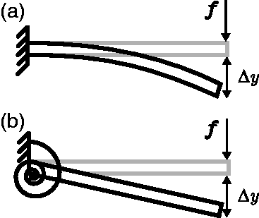
More detailed stiffness analysis methods also consider the finite stiffness of links. Symbolic expressions of structural stiffness matrices are typically developed using a combination of linear beam theory and the rules for addition of elastic elements in series and parallel. The variation lies in the implementation. If compliant parallel manipulators are concerned, the implementation is relatively straightforward, because the Cartesian stiffness matrices of individual legs are invertible.^8,9 However, if a leg contains zero stiffness joints, the Cartesian stiffness matrix of that leg will be singular. Therefore, often only the stiffness along the actuated load vector is considered.^19–21 In the Virtual Joint Method (VJM), this is achieved through a lumped representation of the elasticity in links by virtual joints (see Figure 1).²² The VJM has also been applied to represent the stiffness in constrained directions of lower mobility parallel manipulators with a properly constrained passive leg.^23,24 Using a comparable approach of stiffness mapping, Li and Xu²⁵ included the stiffness in constrained directions for a 3-PUU manipulator. A method that uses the VJM to analyse the stiffness of a general lower mobility parallel manipulators was developed by Pashkevich et al.²⁶

Figure 1.

(a) The finite compliance of a link results in a deformation under loading. (b) In the Virtual Joint Method, this distributed compliance is lumped and represented by a virtual spring with equivalent stiffness.

However, the method by Pashkevich et al. has its shortcomings. The first is that many of the introduced virtual joint coordinates are dependent. As a result, their method requires inversion of relatively large matrices, which is computational expensive. Methods to alleviate the computational burden were proposed by Klimchik et al.,²⁷ but at the expense of an additional implementation effort. Second, the effect of an external load applied at the end-effector is not considered in this method.

This paper aims to develop a stiffness analysis method that is valid for lower mobility manipulators, and which considers the presence of compliant joints, the finite stiffness of links, and also recognises the effect of an applied load. The structure of this paper is as following. First, a novel Jacobian-based stiffness analysis method will be developed. Next, the developed stiffness analysis method will be applied to a 3-RRR mechanism as an example. Finally, the analysis will be simplified for several specific cases, followed by a discussion on the limitations of the presented analysis method.

Analysis

In this section, a stiffness analysis method will be developed, starting from the static equilibrium equation. Insights from Jacobian analysis methods will be used to deal with the possible presence of zero stiffness joints.

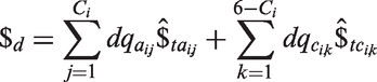
A parallel manipulator consists of multiple serial chains (in this paper referred to as legs) that connect the same end-effector to an inertial base. The displacement twist of the end-effector is defined as $ $d = [d φ ⊤ d p ⊤] ⊤$ , where $d φ$ and $d p$ are the differential rotational and linear displacements of the end-effector, considered at the point that coincides with the origin of a defined Cartesian end-effector reference frame.

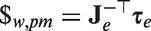
The wrench whose transpose maps $ $d$ on the scalar field of work is $w = [m ⊤ f ⊤] ⊤$ , where $m$ is a moment applied on the end-effector at the point that coincides with the origin of the Cartesian end-effector reference frame and $f$ is a force applied to the end-effector. In a static equilibrium

w, pm = - w, ext

(1)

where $

w, ext

is the net wrench applied on the end-effector by the environment and $

w, pm

is the net wrench applied on the end-effector by all legs of the parallel manipulator, so

w, pm = \sum i = 1 N w, i

(2)

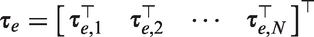
where $

w, i

is the wrench applied on the end-effector by leg i, for a parallel manipulator with N legs.

In the remainder of this section, first the basic assumptions are listed. Next, an existing Jacobian analysis method is used to express joint torques as a wrench in the defined Cartesian end-effector reference frame. A derivation of this wrench then leads to an expression for the Cartesian stiffness matrix.

Basic assumptions

In the analysis presented in this paper, several assumptions are made. First, it is assumed that the manipulator is in a static equilibrium and that all wrenches exerted by the parallel manipulator on the end-effector are caused by elastic deformations, and therefore are all conservative. As such, actuators are modelled as springs, which means that proportional control is assumed to dominate the actuator torque. All other wrenches acting on the end-effector are combined in a single external wrench.

It is also assumed that the vector $τ$ , which is the vector containing all joint torques in the parallel manipulator, can be determined based on the configuration of the manipulator. This determination is a separate topic and will not be further discussed in this paper.

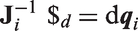
In addition, it is assumed that the parallel manipulator has $0 < F \leq 6$ degrees of freedom (DoFs), with $N \geq F$ . It is further assumed that there are no redundant kinematic joints in each leg (see Wang and Gosselin²⁸ for an example of a parallel manipulator with redundant joints). Then, the number of 1-DoF joints in leg i is equal to its number of kinematic DoFs, which Joshi and Tsai²⁹ refer to as the leg’s connectivity, C_i.

Finally, while the finite structural stiffness of the legs will be included in the analysis, it is assumed that the end-effector body and the inertial body are rigid.

Full inverse Jacobian analysis

Typically, the various wrenches $w, i$ in equation (2) are not directly available, but are obtained by transforming a vector $τ i$ , which is the vector containing all joint torques in leg i of the parallel manipulator. A Jacobian matrix is used to transform $τ i$ into $ $w, i$ . Here we will briefly summarise the Jacobian analysis presented by Huang et al.,³⁰ which is an extension of work by Joshi and Tsai.²⁹ The method is based on screw theory and uses the reciprocity of twists and wrenches to define a set of six linearly independent twists and a set of six linearly independent wrenches. Earlier, a similar method was developed by Ling and Huang,³¹ but due to its more intuitive interpretation, this paper will use the method developed by Huang et al.³⁰

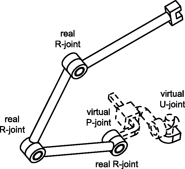
Each of the linearly independent twists maps a single joint velocity onto end-effector Cartesian space. With the assumptions made earlier in this paper, C_i of these twists can be associated with joints that are physically present in the leg. These twists are referred to as the twists of permission. Another $6 - C i$ twists are referred to as the twists of restriction and are associated with the constrained directions. Because twists describe the instantaneous motion along a screw axis, the twists of restriction allow the constrained directions of a leg to be presented by a set of instantaneous virtual, locked joints. This is illustrated for the example of a 3-RRR leg in Figure 2. Because the end-effector is the terminal link of each individual leg, the end-effector displacement twist can be expressed as

d = \sum j = 1 C i dq a i, j \land ta i, j + \sum k = 1 6 - C i dq c i, k \land tc i, k

(3)

where

\land ta i, j

is the twist of permission that maps a unit differential displacement of the

j th

real joint of leg i onto

d

, with

dq a i, j

its intensity. The unit twist of restriction

\land tc i, k

maps the unit differential displacement of the

k th

virtual joint of leg i onto

d

, with intensity

dq c i, k

Figure 2.

The constraints imposed by a leg can be represented by a set of virtual, locked joints, here illustrated for a 3-RRR leg.

Together, these unit twists of permission and unit twists of restriction form a set of six linearly independent unit twists. Such set can be defined for any non-redundant leg, including those of lower mobility parallel manipulators. The unit twists of restriction are generally not unique, but Huang et al.³² describe how unique solutions can be found through the introduction of some simple additional conditions, which hold for most existing parallel manipulators.

Additionally, a set of six linearly independent unit wrenches can be defined, where each unit wrench is associated with a single joint. Each of these wrenches is reciprocal to all twists in equation (3) except one. Therefore, for each leg C_i unit wrenches of actuation can be found, where each unit wrench of actuation is associated to a separate real joint. Another $6 - C i$ unit wrenches can be found which are each associated with one of the virtual joints, and are termed unit wrenches of constraint.

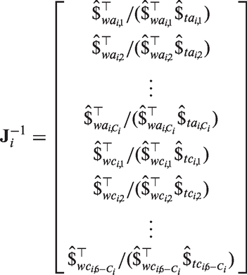
Based on the reciprocity relations between the defined twists and wrenches, left-multiplication of both sides of equation (3) with the transpose of each of the unit wrenches of actuation and unit wrenches of constraint leads to the inverse Jacobian matrix³⁰

J i - 1 d = d q i

(4)

with

\dim (q i) = 6

(5)

and

J i - 1 = [\land wa i, 1 ⊤ / (\land wa i, 1 ⊤ \land ta i, 1) \land wa i, 2 ⊤ / (\land wa i, 2 ⊤ \land ta i, 2) : \land wa i, C i ⊤ / (\land wa i, C i ⊤ \land ta i, C i) \land wc i, 1 ⊤ / (\land wc i, 1 ⊤ \land tc i, 1) \land wc i, 2 ⊤ / (\land wc i, 2 ⊤ \land tc i, 2) : \land wc i, 6 - C i ⊤ / (\land wc i, 6 - C i ⊤ \land tc i, 6 - C i)]

(6)

where

\land wa i, j

is the unit wrench of actuation associated with the

j th

real joint, while

\land wc i, k

is the unit wrench of constraint associated with the

k th

virtual joint of leg i. See Huang et al.³⁰ for more details.

The inverse Jacobian matrix presented in equation (6) transforms the end-effector displacement twist into a vector containing the differential displacements of all joints of leg i, both real and virtual. Because each row in $J i - 1$ maps the end-effector displacement twist onto one differential joint displacement, a given order in which the differential joint displacements appear in $d q i$ determines the order of the rows in $J i - 1$ , or vice versa. The inverse Jacobian expressed by equation (6) is a 6 × 6 matrix and will be referred to as the full inverse Jacobian of leg i. It is a function of the instantaneous configuration of the parallel manipulator.

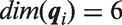
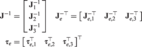
Equation (4) applies to each individual leg, so that for the complete parallel manipulator it holds that

J - 1 d = d q

(7)

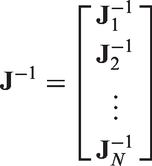
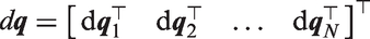
with

J - 1 = [J 1 - 1 J 2 - 1 : J N - 1]

(8)

d q = [d q 1 ⊤ d q 2 ⊤ \dots d q N ⊤] ⊤

(9)

where

J - 1

is the full inverse Jacobian of the parallel manipulator and

d q

is the vector that contains all differential joint displacements. As such,

q

is the vector containing all joint coordinates, both real and virtual, with

\dim (q) = 6 N

Jacobian of elasticity for parallel manipulator

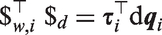
Because the work delivered by each leg is independent of the coordinate frame in which it is expressed

w, i ⊤ d = τ i ⊤ d q i

(10)

where

τ i

is thus the vector that maps

d q i

onto work. Combination of equations (4) and (10) results in

w, i ⊤ d = τ i ⊤ J i - 1 d

(11)

and therefore

w, i = J i - ⊤ τ i

(12)

where the order of the joints associated to the torques in

τ i

is thus equal to that of

d q i

In this paper, all joints of the parallel manipulator are modelled as springs. However, different joints have different properties:

actuated joints have a stiffness that is controllable. The joint torque transferred by an actuated joint is τ_a, which depends on its position, q_a, with respect to a controllable reference position.

passive, compliant joints have a finite stiffness that depends on the specific design. This type of joint transfers a joint torque τ_pc, related to its position q_pc with respect to its unloaded position.

passive, zero stiffness joints are not capable of transferring a torque, so $τ pz = 0$ for all positions q_pz. An example of a joint that can be modelled as a zero stiffness joint is a ball-bearing joint.

virtual joints are a representation of the directions in which the leg is constrained. They represent the instantaneous motion directions which are not permitted by the kinematic model, but which are feasible in practice due to the finite structural stiffness of joints and links. Then, the equivalent joint torque τ_c represents the elastic force resulting from a deformation that can be represented by a deflection dq_c of the virtual joint. Because the virtual joints themselves are mere constructs, as was illustrated in Figure 2, they have no physical properties and are represented in the kinematic model as locked joints, i.e. as joints with infinite stiffness, or zero compliance.

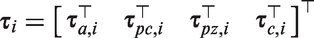
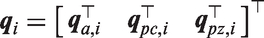
Since the order in which joints appear in the joint coordinate vector is arbitrary, we can define

q i = [q a, i ⊤ q pc, i ⊤ q pz, i ⊤ q c, i ⊤] ⊤

(13)

Because equation (10), this also determines

τ i = [τ a, i ⊤ τ pc, i ⊤ τ pz, i ⊤ τ c, i ⊤] ⊤

(14)

The torque transferred by the zero stiffness joints is zero at all times, so if a leg contains Z_i zero stiffness joints, then $τ pz, i = 0 Z i \times 1$ . This means that the equivalent wrench in Cartesian end-effector space does not depend on $τ pz, i$ and equation (12) can also be written as

w, i = J e, i - ⊤ τ e, i

(15)

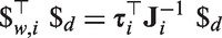
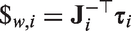
where

τ e, i = [τ a, i ⊤ τ pc, i ⊤ τ c, i ⊤] ⊤

(16)

and

J e, i - 1

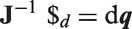
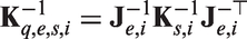
is termed the inverse Jacobian of elasticity. It is obtained from

J i - 1

, expressed in equation (6), by removing the rows associated to the zero stiffness joints. With this definition, it holds that

J e, i - 1 d = d q e, i

(17)

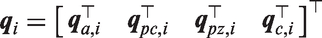
with

d q e, i = [d q a, i ⊤ d q pc, i ⊤ d q c, i ⊤] ⊤

(18)

where

q e, i

is thus the vector containing all joint coordinates of leg i except those of the zero stiffness joints. The components of the vector

q e, i

will be referred to as the elastic joint coordinates of leg i and its associated unit twists are said to span the elastic joint space.

Earlier we concluded that if a leg contains C_i real joints, the number of virtual joints is $6 - C i$ , so that $\dim (q c, i) = 6 - C i$ . If we now consider a leg with A_i actuated joints and Z_i zero stiffness joints, then $\dim (q a, i) = A i$ , $\dim (q pz, i) = Z i$ , and thus $\dim (q pc, i) = C i - A i - Z i$ . As a result

\dim (q e, i) = \dim (τ e, i) = 6 - Z i

(19)

and

J e, i - 1

is a

(6 - Z i) \times 6

matrix.

Because the wrench that is applied by each leg on the end-effector is expressed by equation (15), equation (2) can be rewritten in the form

w, pm = J e - ⊤ τ e

(20)

where

J e - ⊤ = [J e, 1 - ⊤ J e, 2 - ⊤ \dots J e, N - ⊤],

(21)

τ e = [τ e, 1 ⊤ τ e, 2 ⊤ \dots τ e, N ⊤] ⊤

(22)

Equation (20) thus expresses the net wrench applied by the legs of the parallel manipulator on the end-effector as a function of the instantaneous configuration of the parallel manipulator and the torques of all joints except those with zero stiffness.

Stiffness analysis

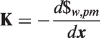
Following the standard definition of positive stiffness, where a displacement results in an opposing force, the Cartesian stiffness matrix of the manipulator is obtained by taking the negative of the derivative of $w, pm$ with respect to the six basis vectors of Cartesian space

K = - \frac{d w, pm}{d x}

(23)

where K is the Cartesian stiffness matrix of the end-effector body relative to the inertial base, expressed in the end-effector reference frame. This 6 × 6 tensor can only be defined if the end-effector can indeed be displaced along all six basis vectors of Cartesian space.³³ In this paper, the finite stiffness of the structural elements of a parallel manipulator will be included in the analysis model, which means that the end-effector can be displaced in any direction irrespective of the kinematic DoFs of the manipulator.

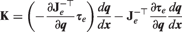
Combination of equation (20) and equation (23) gives

K = - \frac{d (J e - ⊤ τ e)}{d x}

(24)

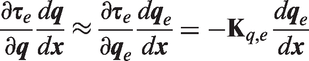
Application of the chain rule then leads to

K = (- \frac{\partial J e - ⊤}{\partial q} τ e) \frac{d q}{d x} - J e - ⊤ \frac{\partial τ e}{\partial q} \frac{d q}{d x}

(25)

Expressions for the required terms in equation (25) are developed below.

Expression for the term $\frac{\partial J e - ⊤}{\partial q} τ e$

As is discussed in more detail by Chen and Kao¹⁶

\frac{\partial J e - ⊤}{\partial q} τ e = [\frac{\partial J e - ⊤}{\partial q 1, 1} τ e \frac{\partial J e - ⊤}{\partial q 1, 2} τ e \dots \frac{\partial J e - ⊤}{\partial q N, 6} τ e]

(26)

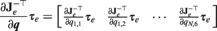
where in this case each term

(\partial J e - ⊤) / (\partial q i, m) τ e

is a 6 × 1 column vector, with

i = 1 \dots N

, and where

q i, m

is the

m th

element of the vector defined in equation (13).

Expression for the term $\frac{\partial τ e ⊤}{\partial q} \frac{d q}{d x}$

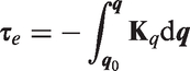
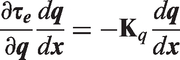
Because all joint torques, including those associated to the virtual joints, are assumed to be the result of elastic deformations, we can express $τ e$ as

τ e = - \int q 0 q K q d q

(27)

where

K q

is the stiffness matrix which maps a differential joint displacement vector

d q

onto a differential joint torque vector

d τ e

. Using equation (27) and the Leibniz integral rule

\frac{\partial τ e}{\partial q} \frac{d q}{d x} = - K q \frac{d q}{d x}

(28)

In traditional stiffness analyses, in which links are assumed infinitely rigid,

K q

is a diagonal matrix containing the individual joint stiffness values.³⁴ If the finite stiffness of links is also included, this matrix will not be a diagonal matrix and will need to be obtained using a different approach, as is outlined below.

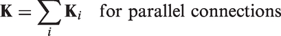
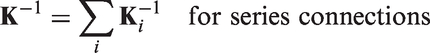
To include the finite stiffness of links in the stiffness analysis, we make use of the stiffness rules for series and parallel connections,

K = \sum_{i} K i for parallel connections

(29)

K - 1 = \sum_{i} K i - 1 for series connections

(30)

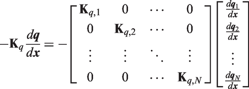
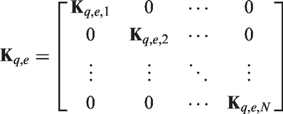
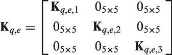
In a parallel manipulator, the matrix K is thus the summation of the stiffness matrices of the individual parallel connections between the inertial base and the end-effector. Since the inertial base and the end-effector were assumed rigid, each of these individual parallel connections is formed by one individual leg. If this summation is expressed in joint space it becomes the block-diagonal concatenation of the stiffness matrices of individual legs, because each leg has its own set of joint coordinates. For a parallel manipulator with N legs, equation (28) can then be written as

- K q \frac{d q}{d x} = - [K q, 1 0 \dots 00 K q, 2 \dots 0 : : : 00 \dots K q, N] [\frac{d q 1}{d x} \frac{d q 2}{d x} : \frac{d q N}{d x}]

(31)

where

K q, i = \frac{\partial τ e, i}{\partial q i}

(32)

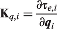
is the stiffness matrix of the

i th

leg, expressed in joint space. It is a tensor that maps a differential joint displacement vector

d q i

onto a differential joint torque vector

d τ e, i

. Because equations (5) and (19), each tensor

K q, i

is a

(6 - Z i) \times 6

matrix. Thus,

K q, i

is generally not a square matrix.

The fact that $K q, i$ generally is not a square matrix is problematic, because in this paper it will obtained by inverting a matrix $K q, i - 1$ . The inverse of stiffness is called compliance, so equation (30) states that the compliance matrix for an individual leg, $K q, i - 1$ , can be constructed by adding the compliance matrices of its serially connected parts. Then, to obtain $K q, i$ , this matrix is inverted and should therefore be a non-singular square matrix.

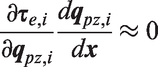
In order to obtain a non-singular square stiffness matrix in joint space, the assumption is made that

\frac{\partial τ e, i}{\partial q pz, i} \frac{d q pz, i}{d x} \approx 0

(33)

which means that the change in joint torques caused by a displacement of a passive, zero stiffness joint as a function of an end-effector deformation is negligible. With this assumption in place,

K q, i

only acts on the vector components of

d q i

associated to joints with a non-zero stiffness. Because in equation (18) the vector that contains these joints was defined as

q e, i

, the assumption presented in equation (33) allows equation (28) to be written as

\frac{\partial τ e}{\partial q} \frac{d q}{d x} \approx \frac{\partial τ e}{\partial q e} \frac{d q e}{d x} = - K q, e \frac{d q e}{d x}

(34)

with

K q, e = [K q, e, 1 0 \dots 00 K q, e, 2 \dots 0 : : : 00 \dots K q, e, N]

(35)

and where each stiffness matrix

K q, e, i

is an invertible

(6 - Z i) \times (6 - Z i)

matrix that acts on

d q e, i

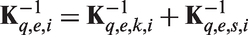
To construct each matrix $K q, e, i$ , equation (30) is used. In this paper, it is chosen to express this equation as a summation of two parts: one part that only includes the compliance of all joints in their kinematic DoF, the kinematic compliance matrix, $K q, e, k, i - 1$ , and another part that represents the structural compliance matrix, $K q, e, s, i - 1$ . Then

K q, e, i - 1 = K q, e, k, i - 1 + K q, e, s, i - 1

(36)

The kinematic compliance matrix,

K q, e, k, i - 1

, is a

(6 - Z i) \times (6 - Z i)

diagonal matrix where each term is the compliance of the respective actuated joint, passive compliant joint or virtual joint. The compliance of actuated and passive compliant joints is real and non-zero, while the compliance of virtual joints is zero, as was earlier discussed. It should be noted that if the zero stiffness joints had not been removed from the analysis, this would have introduced elements of infinite compliance in

K q, e, k, i - 1

. By expressing the compliance matrix in elastic joint space, this problem was effectively avoided.

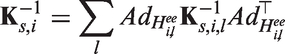
The structural compliance matrix of leg i can be thought of as the leg’s compliance with all kinematic joints locked in place. The matrix $K q, e, s, i - 1$ represents this structural compliance matrix in elastic joint space. This matrix is obtained in two steps. First an expression is obtained of the structural compliance matrix of leg i in end-effector Cartesian space, $K s, i - 1$ . Second, this matrix is mapped onto elastic joint space.

An established method to obtain $K s, i - 1$ is to use adjoint matrices to express the structural compliance matrix of each individual structural element in the Cartesian end-effector reference frame,^8,9,35 so that they can be added as in equation (30). This leads to

K s, i - 1 = \sum_{l} Ad H i, l ee K s, i, l - 1 Ad H i, l ee ⊤

(37)

where

K s, i, l - 1

is the invertible 6 × 6 structural compliance matrix of the

l th

individual structural element of leg i. This matrix is typically expressed in a reference frame connected to the respective structural body, so

Ad H i, l ee

is the 6 × 6 adjoint matrix which transforms a vector from this reference frame into the Cartesian reference frame connected to the end-effector.

Each matrix $K s, i, l - 1$ is a 6 × 6 matrix, so equation (37) forms a $(6 l)$ -dimensional model of the structural compliance of leg i. Next, the transformation

K q, e, s, i - 1 = J e, i - 1 K s, i - 1 J e, i - ⊤

(38)

is used to map

K s, i - 1

onto the elastic joint space of leg i. This transformation enables the addition introduced in equation (36).

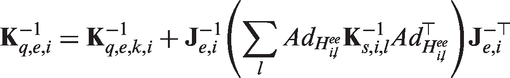
Equations (36) to (38) can be combined into a single expression

K q, e, i - 1 = K q, e, k, i - 1 + J e, i - 1 (\sum_{l} Ad H i, l ee K s, i, l - 1 Ad H i, l ee ⊤) J e, i - ⊤

(39)

It will generally be computationally intensive to invert this symbolic matrix directly and obtain a symbolic expression for

K q, e, i

. A more practical strategy will be to invert

K q, e, i - 1

numerically for a given configuration. From equation (35), it follows that inversion of N matrices, each of dimension

(6 - Z i) \times (6 - Z i)

, is required to obtain an instantaneous numerical expression of matrix

K q, e

Cartesian stiffness analysis

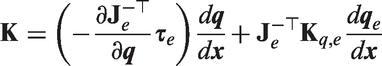
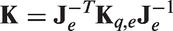
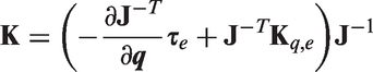
Considering the foregoing derivations and expressions, equation (25) can be rewritten by inserting equation (34), which gives

K = (- \frac{\partial J e - ⊤}{\partial q} τ e) \frac{d q}{d x} + J e - ⊤ K q, e \frac{d q e}{d x}

(40)

Then, because³⁴

\frac{d q}{d x} = J - 1

(41)

and

\frac{d q e}{d x} = J e - 1

(42)

equation (40) can be expressed in the form

K = (- \frac{\partial J e - ⊤}{\partial q} τ e) J - 1 + J e - ⊤ K q, e J e - 1

(43)

where

J - 1

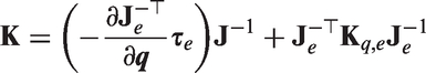
was expressed in (8). Equation (43) is an expression for the Cartesian stiffness matrix of a parallel manipulator with non-redundant legs under loading, which takes the structural stiffness of the legs into account and which is also valid for lower mobility parallel manipulators.*

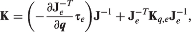
(Inserting the expression $τ e = - J e ⊤ w, ext$ , which follows from equations (1) and (20), and the rule $\frac{\partial J e - ⊤}{\partial q} = - J e - ⊤ \frac{\partial J e ⊤}{\partial q} J e - ⊤$ in equation (43) gives $K = J e - ⊤ K q, e J e - 1 - J e - ⊤ \frac{\partial J e ⊤}{\partial q} w, ext J - 1$ . This equation is equivalent to expressions derived by Chen and Kao¹⁶ and Quennouelle and Gosselin.³⁶ However, since a direct symbolic expression for $J e ⊤$ is typically not available for a parallel manipulator, while such expression is typically available for $J e - ⊤$ , equation (43) is preferred.)

Example analysis of a 3-RRR manipulator

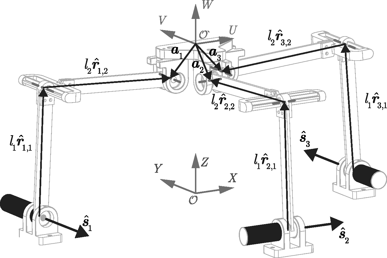
In this section, the introduced stiffness analysis method is applied to a 3-RRR spatial 1-DoF manipulator with three identical legs, shown in Figure 3. The manipulator only allows linear motion along the Z-axis. Each leg consists of an actuated revolute joint (indicated by R), a passive compliant revolute joint and a zero stiffness revolute joint. The spatial manipulator is overconstrained in linear motion along the Y-axis as well as in rotations around the X-axis and the Z-axis. Due to these characteristics, the manipulator presented in Figure 3 is considered as an example of a general parallel manipulator with non-redundant legs.

Figure 3.

A 3-RRR manipulator, where each leg consists of an actuated revolute joint, represented by a filled drum, a passive compliant joint, and a zero stiffness revolute joint. The only kinematically allowed DoF of this spatial 1-DoF manipulator is a translation along the Z-axis.

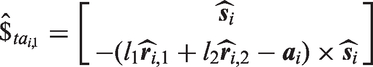
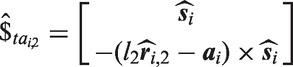
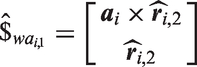
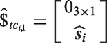
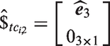
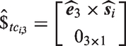
To perform the stiffness analysis, for each leg first a set of six instantaneous, linearly independent unit twists is determined, as well as the unit wrenches which each do work on only one of the unit twists. All twists and wrenches are expressed in a right-handed Cartesian reference frame connected to the end-effector at point $O'$ . The basis vectors of this reference frame are parallel to those of the inertial Cartesian reference frame with origin $O$ . Based on observation of the kinematic structure of an individual leg, and the properties described by Huang et al.,³⁰ the unit twists of permission can be identified as

\land ta i, 1 = [s \land i - (l 1 r \land i, 1 + l 2 r \land i, 2 - a i) \times s \land i]

(44)

\land ta i, 2 = [s \land i - (l 2 r \land i, 2 - a i) \times s \land i]

(45)

\land ta i, 3 = [s \land i a i \times s \land i]

(46)

where

\land ta i, 1, \land ta i, 2

, and

\land ta i, 3

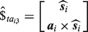
are the unit twists associated to the actuated joint, passive compliant joint, and zero stiffness joint respectively. Furthermore,

s \land 1 = - e \land 2

, which is the unit vector aligned with the negative Y-axis,

s \land 2 = e \land 1

, which is the unit vector aligned with the X-axis, and

s \land 3 = e \land 2

, which is the unit vector aligned with the Y-axis. The other vectors are illustrated in Figure 3, where

r \land i, l

is the unit vector pointing along the

l th

link of leg i and

a \land i

is the vector pointing from

O'

to the center of the third joint of leg i.

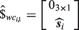
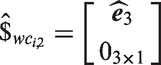
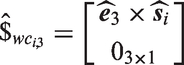
Next, taking the conditions posed by Huang et al.³² into account, a set of wrenches of constraint can also be identified

\land wc i, 1 = [0 3 \times 1 s \land i]

(47)

\land wc i, 2 = [e \land 3 0 3 \times 1]

(48)

\land wc i, 3 = [e \land 3 \times s \land i 0 3 \times 1]

(49)

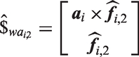
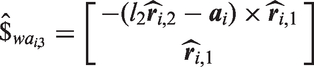
Following the methodology described by Huang et al.,³⁰ these sets of unit twists of permission and unit wrenches of constraint then enable the identification of a set of unit wrenches of actuation

\land wa i, 1 = [a i \times r \land i, 2 r \land i, 2]

(50)

\land wa i, 2 = [a i \times f \land i, 2 f \land i, 2]

(51)

\land wa i, 3 = [- (l 2 r \land i, 2 - a i) \times r \land i, 1 r \land i, 1]

(52)

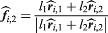
with

f \land i, 2 = \frac{l 1 r \land i, 1 + l 2 r \land i, 2}{| l 1 r \land i, 1 + l 2 r \land i, 2 |}

and finally also a set of unit twists of restriction can be identified

\land tc i, 1 = [0 3 \times 1 s \land i]

(53)

\land tc i, 2 = [e \land 3 0 3 \times 1]

(54)

\land tc i, 3 = [e \land 3 \times s \land i 0 3 \times 1]

(55)

From equations (53) to (55), we can conclude that for each leg the constrained directions can be visualised as a locked prismatic joint, positioned at

O'

and aligned with the vector

s \land i

, and two locked revolute joints, both also positioned at

O'

and aligned with the W-axis and either the U- or V-axis, depending on the leg.

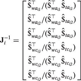
Equations (44) to (55) are then used to obtain the full inverse Jacobian for each leg as in equation (6)

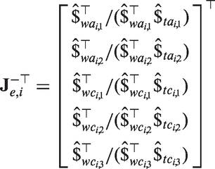
J i - 1 = [\land wa i, 1 ⊤ / (\land wa i, 1 ⊤ \land ta i, 1) \land wa i, 2 ⊤ / (\land wa i, 2 ⊤ \land ta i, 2) \land wa i, 3 ⊤ / (\land wa i, 3 ⊤ \land ta i, 3) \land wc i, 1 ⊤ / (\land wc i, 1 ⊤ \land tc i, 1) \land wc i, 2 ⊤ / (\land wc i, 2 ⊤ \land tc i, 2) \land wc i, 3 ⊤ / (\land wc i, 3 ⊤ \land tc i, 3)]

(56)

Because the third joint in each leg is a zero stiffness joint and the torque transferred by it will be zero at all times, we can remove the associated row from

J i - 1

to form the inverse Jacobian of elasticity, whose transpose

J e, i - ⊤ = [\land wa i, 1 ⊤ / (\land wa i, 1 ⊤ \land ta i, 1) \land wa i, 2 ⊤ / (\land wa i, 2 ⊤ \land ta i, 2) \land wc i, 1 ⊤ / (\land wc i, 1 ⊤ \land tc i, 1) \land wc i, 2 ⊤ / (\land wc i, 2 ⊤ \land tc i, 2) \land wc i, 3 ⊤ / (\land wc i, 3 ⊤ \land tc i, 3)] ⊤

(57)

maps all non-zero torques transferred by leg i from joint space onto end-effector Cartesian space as in equation (15). Since each of the three legs includes one zero stiffness joint, Z_i = 1 for $i = 1 \dots 3$ .

Because $Z i \neq 0$ , the stiffness matrix of leg i, expressed as $K q, i$ in equation (32) is not a square matrix. We will therefore make use of the assumption expressed in equation (33). The resulting stiffness matrix $K q, e, i$ for each individual leg is invertible and can be developed using equations (36) to (38).

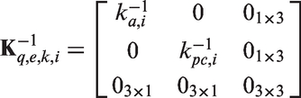
Equation (39) expresses $K q, e, i - 1$ as a function of the matrices $K q, e, k, i - 1$ and the compliance matrices of individual structural elements $K s, i, l - 1$ . Using equation (16), and because virtual joints are modelled with zero compliance

K q, e, k, i - 1 = [k a, i - 1 0 0 1 \times 3 0 k pc, i - 1 0 1 \times 3 0 3 \times 1 0 3 \times 1 0 3 \times 3]

(58)

where

k a, i

is the actuator stiffness and

k pc, i

is the stiffness of the compliant joint of leg i. The symbolic matrices

K s, i, l - 1

can be developed using linear beam theory^8,9 as discussed earlier, and will not be described in further detail in this paper.

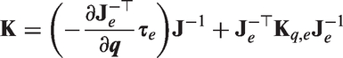
With above expressions, the Cartesian stiffness matrix can be obtained from equation (43), which is repeated here for convenience

K = (- \frac{\partial J e - ⊤}{\partial q} τ e) J - 1 + J e - ⊤ K q, e J e - 1

where for this example

J - 1 = [J 1 - 1 J 2 - 1 J 3 - 1] J e - ⊤ = [J e, 1 - ⊤ J e, 2 - ⊤ J e, 3 - ⊤] τ e = [τ e, 1 ⊤ τ e, 2 ⊤ τ e, 3 ⊤] ⊤

with

J i - 1

defined by equation (56),

J e, i - ⊤

by equation (57), and

τ e, i = [τ a, i τ pc, i τ c, i, 1 τ c, i, 2 τ c, i, 3] ⊤

For the presented example,

τ a, i

is controlled,

τ pc, i

can be determined from the manipulator configuration and the properties of the implemented compliant joint, while

τ c, i, j = 0

if the individual legs are not loaded in their respective constrained directions. Finally, the matrix

K q, e

is obtained using equation (35) as

K q, e = [K q, e, 1 0 5 \times 5 0 5 \times 5 0 5 \times 5 K q, e, 2 0 5 \times 5 0 5 \times 5 0 5 \times 5 K q, e, 3]

where each matrix

K q, e, i

can thus be obtained by (numerically) inverting the symbolically expressed matrix

K q, e, i - 1

, which was expressed in equation (39).

Thus, all partial matrices necessary to determine K are directly available in symbolic form, except $K q, e$ , which would in this example require the numerical inversion of three 5 × 5 matrices.

Discussion

The presented Jacobian-based stiffness analysis method applies to a general parallel manipulator with non-redundant legs in a loaded condition and takes both joint compliance and structural compliance into account. Comparable existing analysis methods were either developed for more specific manipulators or did not consider loading, which makes the presented analysis method more complete.

Besides its completeness, the presented method has two implementation advantages over comparable existing methods. The first advantage is that the matrices that need to be inverted are relatively small. To obtain the stiffness matrix of individual legs requires an inversion of the corresponding compliance matrix. In the method by Pashkevich et al.,²⁶ each of these matrices is of size $(6 + Z i) \times (6 + Z i)$ , while in the presented method they are $(6 - Z i) \times (6 - Z i)$ matrices. This size reduction is likely to result in a computational advantage.

The second advantage of the presented analysis is that despite its completeness, its structure allows for easy simplifications if desired. This makes the presented analysis very flexible. To demonstrate this, three possible simplifications are discussed here.

No loading

In case of no loading, $τ e = 0$ . Then, the first term after the equal sign in equation (43) is zero and the stiffness analysis reduces to

K = J e - T K q, e J e - 1

(59)

which is the transformation of the stiffness matrix from elastic joint space to Cartesian space.

It should be noted that $τ e = 0$ is not the same as $w, pm = 0$ . From equation (2), it can be concluded that the latter only means that the net wrench is zero, which allows for situations where the wrenches applied by individual legs are finite, but cancel each other out. In that case internal loading occurs and $τ e \neq 0$ . Thus, a parallel manipulator can be in a loaded condition, even if no external wrench is applied to the end-effector.

Infinite structural stiffness

If the structural stiffness is assumed infinite, the Cartesian stiffness matrix can only be defined if none of the individual legs of a parallel manipulator are structurally constrained, so for a 6-DoF parallel manipulator. This is because K is only well defined if the end-effector can be displaced along all six basis vectors of Cartesian space. This is not the case for lower mobility manipulators with a structural stiffness that is assumed infinite, because in that case the modelled stiffness in the constrained directions is infinite.

However, if none of the individual legs of a parallel manipulator are structurally constrained (e.g. a Stewart platform), the vector $q c, i$ is the zero vector and the configuration of each leg is defined by the vector which contains all real, kinematic joint coordinates

q i = [q a, i ⊤ q pc, i ⊤ q pz, i ⊤] ⊤

(60)

For this class of manipulators, the Cartesian stiffness matrix is again expressed by equation (43)

K = (- \frac{\partial J e - T}{\partial q} τ e) J - 1 + J e - T K q, e J e - 1,

where the stiffness matrix

K q, e

is expressed by equation (34). However, without elasticity in the structural elements,

K q, e, s, i - 1 = 0

for each leg and thus

K q, e

is simply the diagonal matrix containing the stiffness values of all actuated joints and passive, compliant joints of the manipulator.

Compliant parallel manipulator

Compliant parallel manipulators are parallel manipulators which do not contain any passive, zero stiffness joints. Instead, all passive joints are compliant joints. In these compliant parallel manipulators, the vector $q pz, i$ is the zero vector for all legs and therefore

q i = [q a, i ⊤ q pc, i ⊤ q c, i ⊤] ⊤

(61)

so that

J e, i - T = J i - T

(62)

In this case, equation (43) simplifies to

K = (- \frac{\partial J - T}{\partial q} τ e + J - T K q, e) J - 1

(63)

Complications and limitations

Although the presented analysis method is valid for a general parallel manipulator with non-redundant legs, there are several factors which may complicate this analysis or limit its use. First, it is assumed that all joint torques are known, including those associated to the virtual joints. Especially if a parallel manipulator is overconstrained, there may be additional difficulties in determining the constraint torques.

Second, because both the Jacobian and the structural stiffness matrices are linear approximation, appropriate care should be taken if the presented stiffness analysis method is used to quantitatively assess displacements as a result of external loads. Especially if the parallel manipulator is close to a singularity or if displacements under loading become relatively large, the predicted displacements will likely be less accurate.

Another limitation comes from the fact that we assumed the end-effector itself to be rigid. Thus, users of this analysis method should verify that the compliance of the end-effector body is indeed negligible.

Finally, if a parallel manipulator contains zero stiffness joints and the finite stiffness of structural elements is included in the stiffness analysis, the assumption presented in equation (33) was made. Although we consider it very unlikely that a deflection of a passive, zero stiffness joint as a function of an end-effector deflection causes a significant change in elastic joint torques, users of the presented analysis should keep this assumption in mind.

Conclusion

This paper has presented a novel Jacobian-based stiffness analysis method for parallel manipulators with non-redundant legs, based on the static equilibrium equation. Because parallel manipulators often interact with an environment, an external wrench acting on the end-effector was included in this equilibrium equation. The method is valid for both 6-DoF and lower mobility manipulators, and it considers the presence of compliant joints and the finite stiffness of links.

The presented analysis uses an existing method based on screw theory to define for each leg a set of six linearly dependent, instantaneous joint axes. Each axis is associated to an actuated joint, a passive compliant joint, a zero stiffness joint, or a virtual joint. Virtual joints represent the motion restricted by the kinematic joints of the leg in question. The four different types of joints have different stiffness properties and therefore affect the resulting end-effector stiffness in different ways. The joint coordinates associated to actuated, passive flexure, and virtual joints are together referred to as elastic joint coordinates.

The method presented in this paper integrates a symbolic structural stiffness analysis method based on adjoint matrices with a stiffness analysis method that relies on the transformation between a joint space and a Cartesian space. The resulting method is also valid for parallel manipulators with zero stiffness joints, because this method uses a mapping of the 6 × 6 structural stiffness matrix of a leg into the space spanned by its elastic joint coordinates. The resulting matrix of reduced dimension can be inverted.

To demonstrate the presented stiffness analysis method, it has been applied to a spatial 1-DoF parallel manipulator. Additionally, to illustrate the generality of the method, three specific cases were discussed. One case assumed the absence of loading, another infinite structural stiffness, and a third considered the stiffness analysis of a compliant parallel manipulator. The presented Cartesian stiffness analysis method therefore generalises much of the existing Jacobian-based stiffness analysis methods for parallel manipulators with non-redundant legs.

Footnotes

Declaration of conflicting interests

The author(s) declared no potential conflicts of interest with respect to the research, authorship, and/or publication of this article.

Funding

The author(s) disclosed receipt of the following financial support for the research, authorship, and/or publication of this article: This work was supported by the Dutch Technology Foundation STW (project number 12158).

References

Merlet

. Parallel robots. Solid mechanics and its application, 2nd ed. Dordrecht: Springer, 2006.

Wei

Simaan

. Design of planar parallel robots with preloaded flexures for guaranteed backlash prevention. J Mech Robot 2010; 2: 011012–011012.

Borras J and Dollar AM. Static analysis of parallel robots with compliant joints for in-hand manipulation. In: IEEE/RSJ international conference on intelligent robots and systems. New York: IEEE, 2012, pp.3086–3092.

Kang D and Gweon D. Analysis of large range rotational flexure in precision 6-DOF tripod robot. In: 12th International conference on control, automation and systems (ICCAS). New York: IEEE, 2012, pp.2117–2120.

Clinton CM, Zhang G and Wavering AJ. Stiffness modeling of a Stewart platform based milling machine. Technical Report, ISR. http://hdl.handle.net/1903/5859 (1997, accessed 7 August 2015).

Company

Krut

Pierrot

. Modelling and preliminary design issues of a four-axis parallel machine for heavy parts handling. Proc IMechE, Part K: Journal of Multi-body Dynamics 2002; 216: 1–12.

Zhang

Song

. Stiffness modeling and analysis of a novel 4-DOF PKM for manufacturing large components. Chin J Aeronaut 2013; 26: 1577–1585.

Pham

Chen

. Stiffness modeling of flexure parallel mechanism. Precis Eng 2005; 29: 467–478.

Dai

Ding

. Compliance analysis of a three-legged rigidly-connected platform device. J Mech Des 2006; 128: 755–755.

10.

Raatz

Wrege

Burisch

Compliant parallel robots. In: Ratchev

(ed). Precision assembly technologies for mini and micro products, Boston: Springer US, 2006, pp. 83–92.

11.

Dong

Sun

. Stiffness research on a high-precision, large-workspace parallel mechanism with compliant joints. Precis Eng 2008; 32: 222–231.

12.

Yue

Gao

Zhao

. Relationship among input-force, payload, stiffness, and displacement of a 6-DOF perpendicular parallel micromanipulator. J Mech Robot 2010; 2: 011007–011007.

13.

Gao

Zhang

. Simulation driven performance characterization of a spatial compliant parallel mechanism. Int J Mech Mater Des 2014; 10: 227–246.

14.

Salisbury

Craig

. Articulated hands: force control and kinematic issues. Int J Robot Res 1982; 1: 4–17.

15.

Gosselin

. Stiffness mapping for parallel manipulators. IEEE Trans Robot Automat 1990; 6: 377–382.

16.

Chen

Kao

. Conservative congruence transformation for joint and Cartesian stiffness matrices of robotic hands and fingers. Int J Robot Res 2000; 19: 835–847.

17.

Alici

Shirinzadeh

. Enhanced stiffness modeling, identification and characterization for robot manipulators. IEEE Trans Robot 2005; 21: 554–564.

18.

Quennouelle

Gosselin

. A quasi-static model for planar compliant parallel mechanisms. J Mech Robot 2009; 1: 021012–021012.

19.

Huang

Zhao

Whitehouse

. Stiffness estimation of a tripod-based parallel kinematic machine. IEEE Trans Robot Automat 2002; 18: 50–58.

20.

Wahle M and Corves B. Stiffness analysis of Clavels DELTA robot. In: Jeschke S, Liu H and Schilberg D (eds) Intelligent robotics and applications. Lecture Notes in Computer Science 7101. Berlin, Heidelberg: Springer Berlin Heidelberg. ISBN 978-3-642-25485-7, 2011, pp.240–249.

21.

Ahmad

Andersson

Sellgren

. A stiffness modeling methodology for simulation-driven design of haptic devices. Eng Comput 2012; 30: 125–141.

22.

Zhang D. Kinetostatic analysis and optimization of parallel and hybrid architectures for machine tools. PhD Thesis, Laval University, Canada, 2000.

23.

Zhang

Lang

. Stiffness modeling for a class of reconfigurable PKMs with three to five degrees of freedom. J Manuf Syst 2004; 23: 316–327.

24.

Wang

Liu

Huang

. Stiffness modeling of the tricept robot using the overall Jacobian matrix. J Mech Robot 2009; 1: 021002–021002.

25.

. Stiffness analysis for a 3-PUU parallel kinematic machine. Mech Mach Theor 2008; 43: 186–200.

26.

Pashkevich

Chablat

Wenger

. Stiffness analysis of overconstrained parallel manipulators. Mech Mach Theor 2009; 44: 966–982.

27.

Klimchik

Pashkevich

Caro

. Stiffness matrix of manipulators with passive joints: computational aspects. IEEE Trans Robot 2012; 28: 955–958.

28.

Wang

Gosselin

. Kinematic analysis and design of kinematically redundant parallel mechanisms. J Mech Design 2004; 126: 109–109.

29.

Joshi

Tsai

. Jacobian analysis of limited-DOF parallel manipulators. J Mech Design 2002; 124: 254–254.

30.

Huang

Liu

Chetwynd

. Generalized Jacobian analysis of lower mobility manipulators. Mech Mach Theor 2011; 46: 831–844.

31.

Ling

Huang

. Kinestatic analysis of general parallel manipulators. J Mech Design 1995; 117: 601–601.

32.

Huang

Yang

Wang

. An approach to determining the unknown twist/wrench subspaces of lower mobility serial kinematic chains. J Mech Robot 2014; 7: 031003–031003.

33.

Zefran M and Kumar V. Affine connections for the Cartesian stiffness matrix. In: Proceedings of international conference on robotics and automation. Vol. 2. New York: IEEE. 1997, pp.1376–1381.

34.

Merlet

Gosselin

. Springer handbook of robotics, Berlin, Heidelberg: Springer Berlin Heidelberg, 2008.

35.

Murray

Sastry

. A mathematical introduction to robotic manipulation, Boca Raton, FL: CRC Press, 1994.

36.

Quennouelle C and Gosselin CM. A general formulation for the stiffness matrix of parallel mechanisms. 2012; arXiv:1212.0950 [physics.class-ph].

Jacobian-based stiffness analysis method for parallel manipulators with non-redundant legs

Abstract

Keywords

Introduction

Analysis

Basic assumptions

Full inverse Jacobian analysis

Jacobian of elasticity for parallel manipulator

Stiffness analysis

Expression for the term ∂ J e - ⊤ ∂ q τ e

Expression for the term ∂ τ e ⊤ ∂ q d q d x

Cartesian stiffness analysis

Example analysis of a 3-RRR manipulator

Discussion

No loading

Infinite structural stiffness

Compliant parallel manipulator

Complications and limitations

Conclusion

Footnotes

Declaration of conflicting interests

Funding

References

Expression for the term $\frac{\partial J e - ⊤}{\partial q} τ e$

Expression for the term $\frac{\partial τ e ⊤}{\partial q} \frac{d q}{d x}$