
Abstract
As a critical part of the analysis of the micro-milling process, mechanical modeling directly affects the prediction of the surface finish of machining materials and the cutting stability. In this paper, a flexible force model of micro-milling is established, which accounts for the influence of the actual cycloid tool path, tool runout, elastic recovery, tool deformation, and chip separation state. The Harris Hawks Error Optimization parameter identification method is proposed to efficiently obtain the cutting force coefficient/parameter. Based on the uncertainty of system parameters caused by the manufacturing and assembly process, probability distribution characteristics of the micro-milling force are predicted and analyzed. Additionally, the Adaptive Kriging method is used to reconstruct the complex implicit relationship between the cutting parameters and milling forces, improving the computational efficiency of the probability analysis. Finally, a series of micro-milling experiments and computational results verified the accuracy of the proposed method.
Keywords
Introduction
With the characteristics of small machining size, a wide range of machinable materials, complex surface machining, and low cost, micro-milling has become an essential technology in the manufacturing fields such as aerospace, biomedical, automotive, electronic, and others, which is the current research hotspot.1–3 However, micro-milling is easily affected by minor variations such as tool deformation and instantaneous cutting thickness. 4 Consequently, understanding and modeling the micro-milling process are critical when aiming to improve the quality of machined parts and production efficiency.
Compared to macro-machining, micro-machining considers problems at a small scale (micro problems), making it difficult to study the underlying micro-milling mechanic mechanisms. Wang et al. 5 redefined and calculated the cutting radius and instantaneous uncut chip thickness in the machining process to predict the cutting force in the micro end milling process. Further, Guo et al. 6 proposed an instantaneous undeformed thickness model for micro-milling considering tool runout, variable pitch, and helix angle. Based on multi-scale modeling and analysis, Niu and Cheng 7 proposed an innovative expression of micro machining cutting force. Next, Liu et al. 8 investigated a micro-milling mathematical model of the thin-walled copper structure and verified the proposed model using finite element simulation. Considering the tool size, tool runout, and spatial tool position, Jing et al. 9 and Zhang et al. 10 established more accurate micro-milling tool runout and instantaneous force models. All of the above-listed models described the micromachining processes under some influencing factors, providing a basis for establishing a more comprehensive micro-milling force model, which will consider multiple related factors.
To create a more accurate cutting force model, the factors such as chip separation state, instantaneous cutting thickness, tool runout, workpiece elastic recovery, effectively included angle, and the interaction between tool deformation and cutting forces are integrated into the modeling. In addition, the accurate and efficient measurement or calculation of the cutting coefficient/parameter in the mechanical model is essential. Gonzalo et al. 11 calculated the specific cutting force coefficient by substituting the identified simulated force and measured force for reverse calculation into the linear mechanics model. Jin and Altintas 12 and Tsai et al. 13 predicted the cutting force coefficient based on the finite element analysis and milling experimental results. By combining experimental measurement with numerical calculation, 14 Li et al. 15 analyzed the ratio of total force corresponding to each cutting edge according to the spatial geometric relationship to determine the tool runout parameters. However, using finite element analysis, cyclic iteration, and experimental methods for calculating cutting the coefficient/parameters is relatively complex and somewhat time-consuming.
Hence, the Harris Hawkes Error Optimization (HEO) method is developed to identify cutting coefficients/parameters both concisely and efficiently. The square difference between the predicted and experimental forces is used to construct the optimization objective function. The process parameters are usually regarded as deterministic variables in the prediction methods of micro-milling force, but these parameters are variable and affect the machining process. 16 Consequently, in this paper, the probability characteristics of the micro-milling force are studied. The Adaptive-Kriging (AK) method is used to reconstruct the functional relationship between the machining parameters and the milling force to improve the calculation efficiency. Comparing the predicted results of the AK method and directly proposed model calculations verify the accuracy of the probabilistic characteristic analysis conclusions.
The paper is structured as follows: a novel comprehensive cutting force model, including the effects above, is proposed in Section 2. In Section 3, the HEO algorithm is presented and used to identify the cutting coefficients/parameters. Section 4 illustrates the AK method used in probability analysis. The experimental device is designed to verify the proposed prediction model and AK model, and the probability distribution characteristics of the micro-milling force are obtained in Section 5. Section 6 summarizes the conclusions of this work.
Mechanical modeling of micro-milling
Chip thickness analysis
The radial variation of the actual cutting point results in periodical changes in the force acting on the cutting edge, which can be defined as tool runout. As shown in Figure 1(a), the existence of runout causes the geometric central axis of the tool to no longer be collinear with the central rotation axis, resulting in the change of the actual tool position and rotation radius. The actual tool rotation radius can be calculated as:
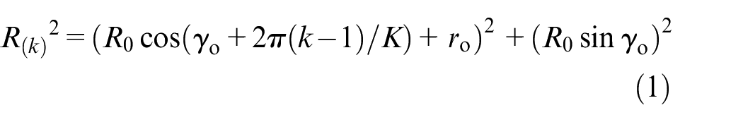
Micro geometric relationship: (a) cutting tool center offset, (b) the geometry calculation of IUCT, and (c) chip formation mechanism.
where R0 is the tool radius, k is the number of the current flute, K is the total number of tools, γo and ro are the runout angle and value. The trajectories O of the tool center are formulated as:
where f is the feed rate, ω is the angular velocity. The trajectory of the kth edge can be written as:
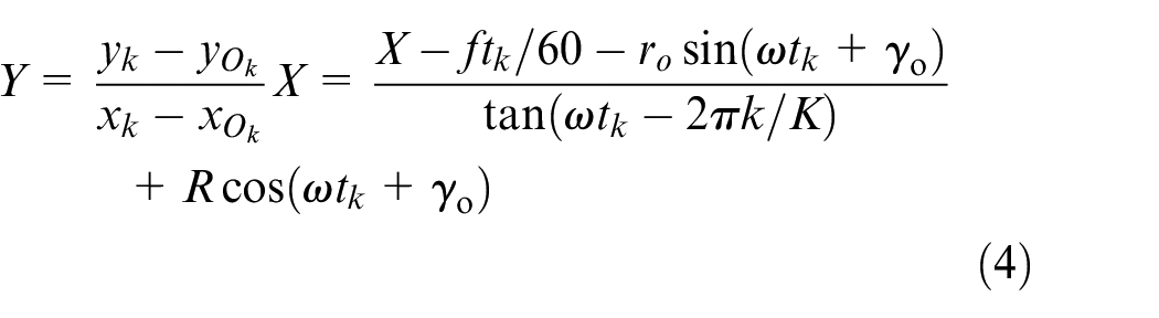
According to the geometric relationship in Figure 1, the kth tooltip can be denoted as M (x, y) with the tool center located at O k . The line MOk can be expressed as follows:
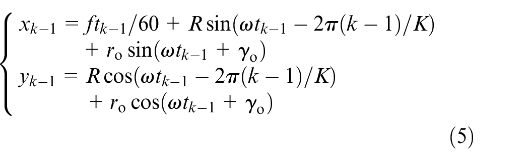
The coordinates of the k−1th cutting edge Mk−1(xk−1, yk−1) are obtained based on the above kth tooth trajectory analysis presented earlier:
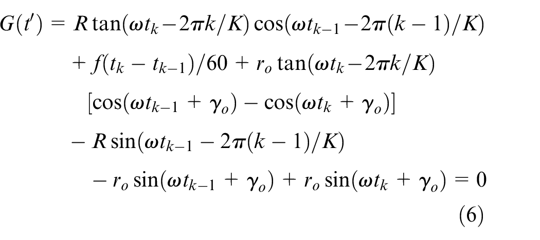
It can be seen from Figure 1(b) that the instantaneous uncut chip thickness (IUCT) is the min-distance of the intersection between the cutting trajectory of the current and the previous tooth. Let Mk−1 be the intersection of the MOk and the k−1th cutting trajectory. Substituting equation (5) into the linear MOk equation of equation (4):
The nonlinear equations related to time t′ are solved by the Newton Raphson iteration method, 17 and the initial time ti iteration update can be expressed as:
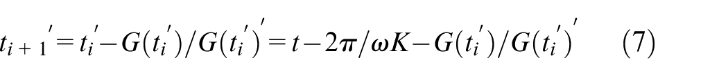
where G(ti′)′ is the first derivative of G(ti′). The flow of solving the IUCT can be derived as follows:
As shown in Figure 1(c), the chips are not formed when the chip thickness is less than the minimum chip thickness (MCT), and part of material elastic recovery except for the chip. The actual IUCT requires superposition calculation, which can be expressed as:
where Pe is the elastic recovery rate of the workpiece, hmin is the MCT, and λ is the experimentally-obtained coefficient. 18 Figure 2 shows the instantaneous cutting thickness curves of two tooth cutters considering different work conditions.
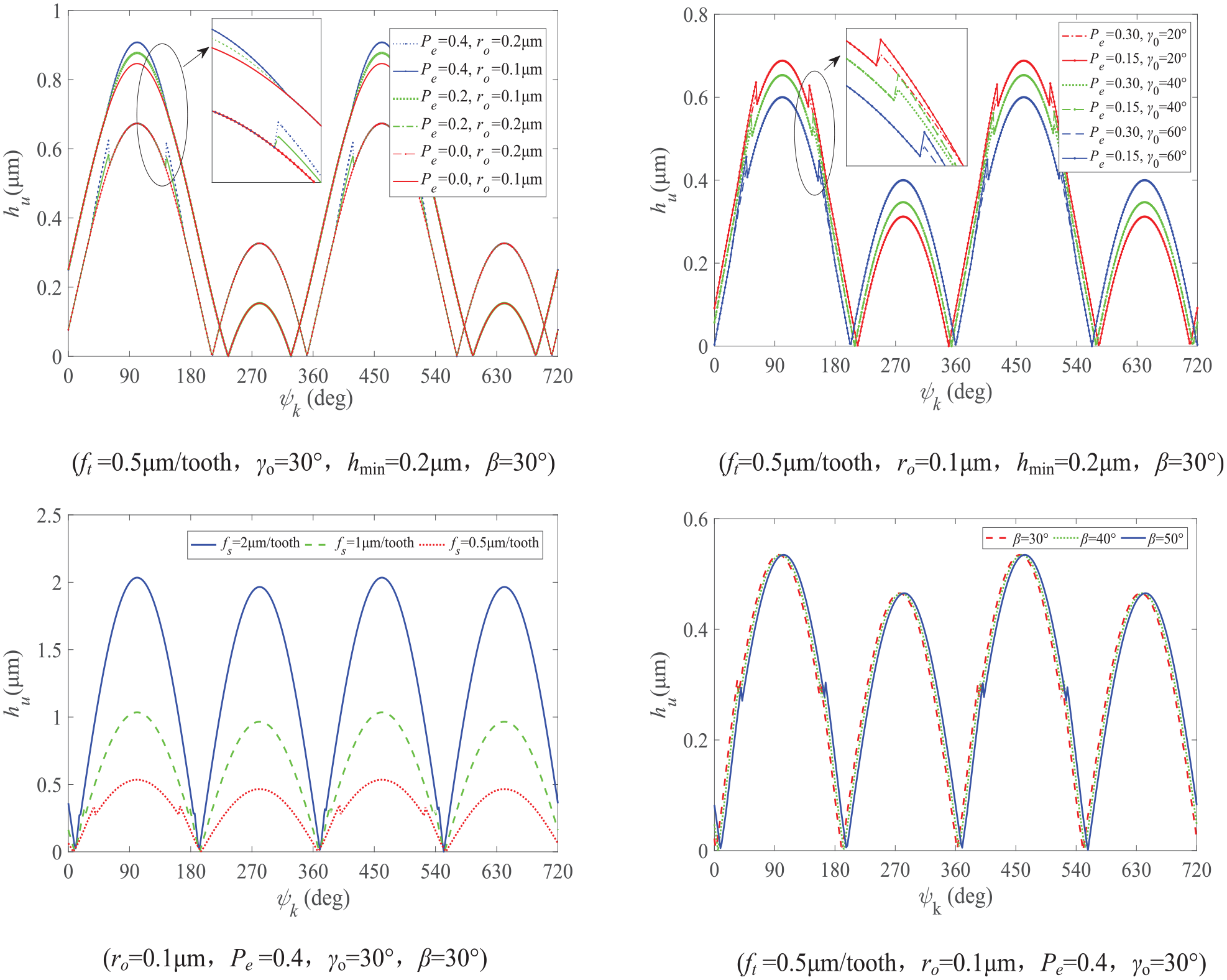
IUCT with different work conditions (ψk is the cutting edge position angle).
Due to the existence of the MCT, the IUCT curve suddenly increases at tooth 1, resulting in a superposition effect, which will gradually disappear as the runout or feed per tooth increases. Moreover, the IUCT increases with the growth of elastic recovery rate (Pe), runout length (ro), and feed per tooth (fs) and decreases with the rise of runout angle (γo). The change of the tool helix angle (β) will change the cutting tool working area, not the size of the IUCT. In addition, the effect of the runout on the instantaneous cutting thickness gradually decreases with the fs increases.
Tool deformation analysis
As shown in Figure 3, the cutting is divided into the shear/plough dominant region (SDR/PDR). The chip flow direction is the same as that of the effective rake angle. The force acting on AC can be expressed as:
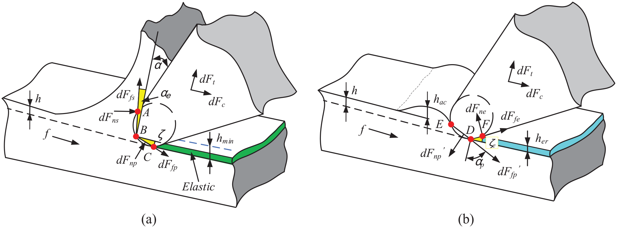
The diagram of the SDR-(a) and RDR-(b).
where Kns and Kfs are the shear cutting coefficients, dz is the height of the cutting edge discrete elements. Through geometric analysis and integration simplification, the instantaneous effective rake angle αe can be written as:
The plough force acting on AB is proportional to the MCT. Its components in the direction of the cutting speed and the radial direction are given as:
where Knp and Kfp are plough coefficients and ζ is the angle between AB and the horizontal plane. As shown in Figure 3(b), the cutting state does not form chips, and the material accumulates at the height hac in front of the blade. The cutting force components can be calculated as:
where αp is the instantaneous rake angle. There is a linear relationship between the height of the accumulation under plowing and the rheological factor 19 :
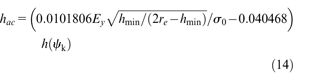
where Ey and σ0 are the Young’s modulus and yield stress of the workpiece. The friction can be decomposed in radial and thrust directions:
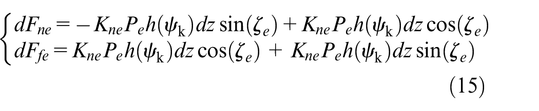
where Kne and Kfe are coefficients of friction. The clearance angle of the blade γ, and the angle ζe can be determined from:
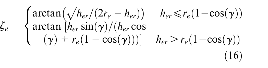
where her is the elastic recovery height. Based on the calculations presented above and after dividing the cutting edge into M sections, the cutting forces in the x and y directions can be written as:
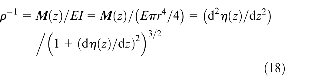
Due to the small tool diameter, the effect of tool deflection on the IUCT in micro-milling should be considered. As shown in Figure 4(a), the tool flute forces are transmitted to the tool shank, which can be regarded as an arc with radius ρ with the action of force/moment (
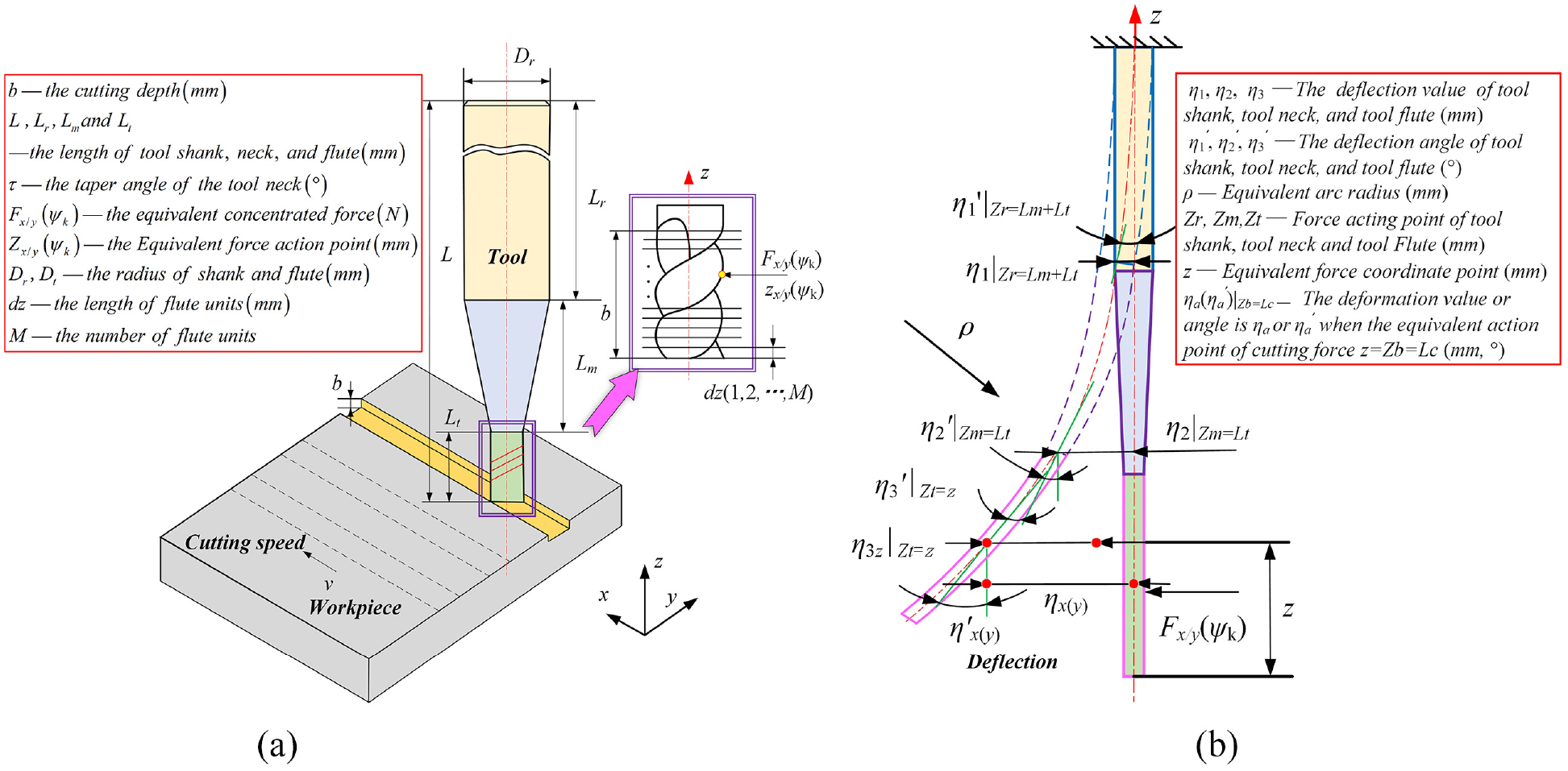
Simplified model of the micro-milling tool: (a) Micro-milling cutting process and (b) Deformation process of micro-milling tool.
where η(z) is the deflection value of the tool, and I is the moment of inertia. The simplified beam deflection and rotation angle equations can be obtained:

The overall force and deformation analysis of the tool are shown in Figure 4(b). The deformation at a point z on the tool flute under the effect of cutting force can be expressed as:
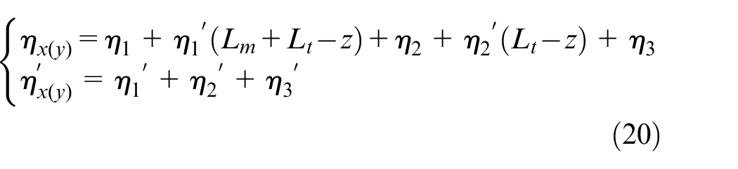
where η1, η1′, η2, η2′, η3, and η3′are the deflection value and angle of the tool shank/neck/flute, which can be calculated by:
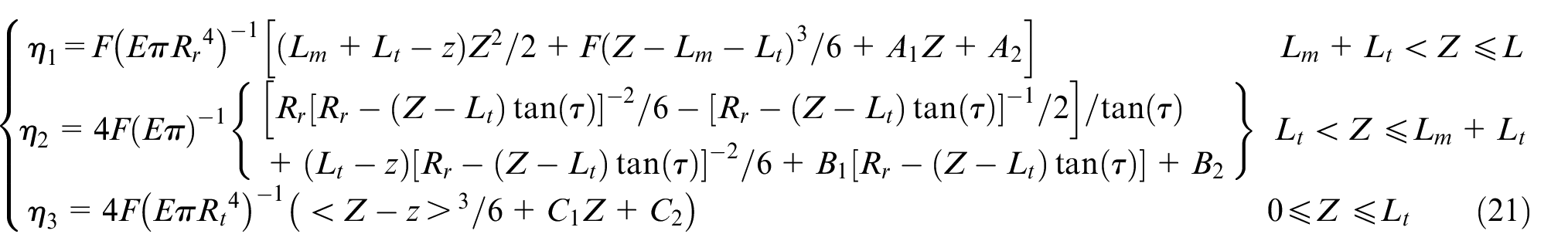
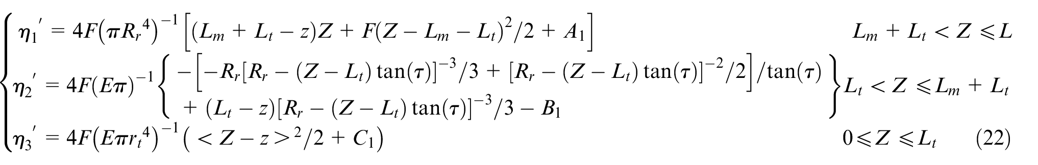
where Rr is the shank radius, τ is the inclination angle, Z is the actual force point on the tool, and z (zx/y(ψk)) is the equivalent force point. By substituting the boundary conditions into equations (21) and (22), the constant value parameters A1, A2, B1, B2, C1, and C2 can be solved. According to the equivalence relationship, the concentrated force moment can be expressed as the sum of the moments of all microelements:
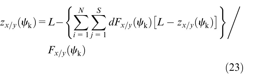
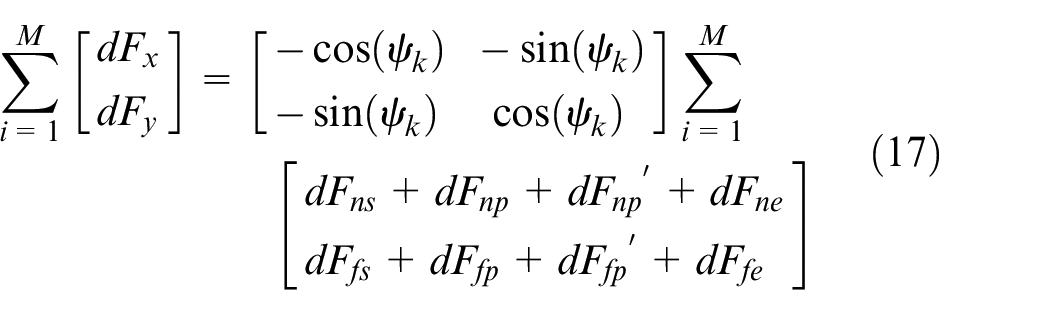
where dFx/y(φ) is the microelement force in the x/y-axis. N and S are the numbers of flute and microelements.
Flexible force model
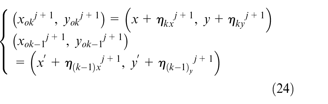
Due to the tool deformation-induced changes in the tooth trajectory and IUCT, the mechanical model must be updated. The current tool deflection value is used to update the position of the next tool center to obtain an accurate tool tip trajectory. As shown in Figure 5, the red and green dotted lines indicate the adjacent tooth tool path before the offset, while the solid lines show its path following the offset. Tooltip paths of the preceding and the current tooth before and after offset are (xkj+1, ykj+1) and (xk−1j+1, yk−1j+1), respectively, while the actual IUCT is designated as hnkj+1. Then the tool center trajectory in actual processing can be expressed as:
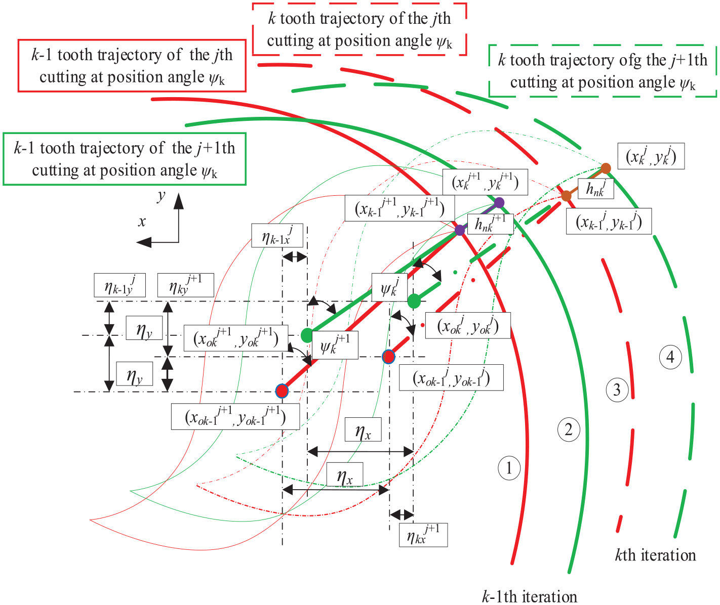
The coordinate change caused by tool deflection.
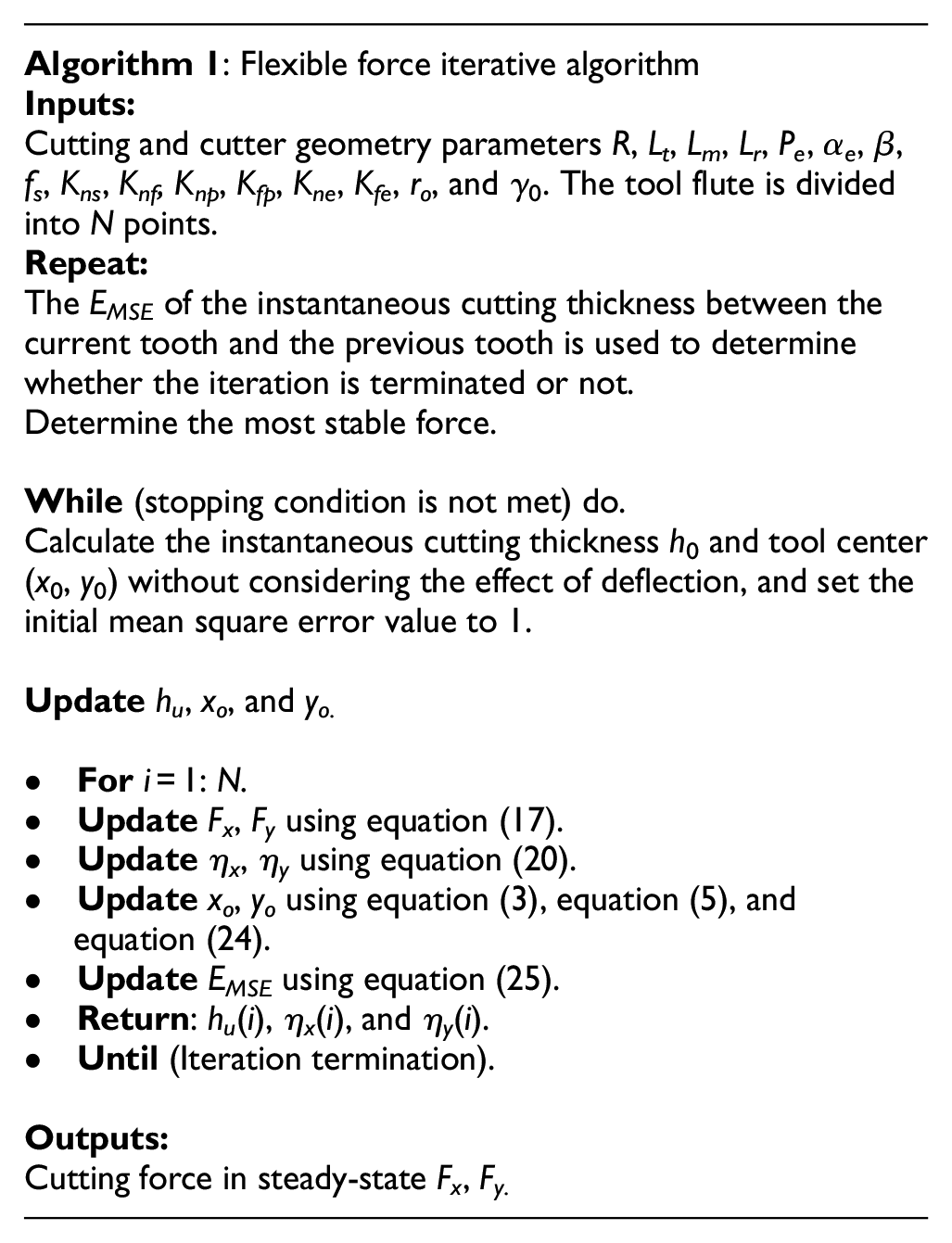
where ηkxj+1, ηkyj+1, η(k−1)xj+1, and η(k−1)yj+1 are the distance of the tool center offset distance, which can be calculated in Section 2.2. The mean square error (MSE) is the difference in the IUCT between consecutive tooth channels. The MSE is measured to evaluate the cutting steady-state and convergence. The iterative discriminant can be expressed as:
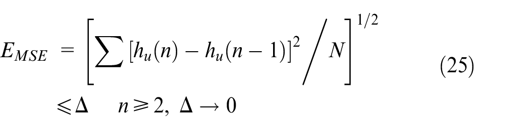
where N is the sample size, n is the number of tooth paths, hu(n) and hu(n−1) are the IUCT removed between the n and n−1 tooth path at the position angle ψk. Once the iteration reaches convergence, the IUCT in the stable-state can be obtained, and the steps of the iterative algorithm are given in Algorithm 1.
Coefficient identification and fitting method
The effective rake and clearance angles are variable parameters for calculating IUCT-h(ψk). Further, the traditional linear fitting and experimental measurement 20 cannot be directly used to obtain parameters. To overcome these shortcomings, the Harris hawks Error Optimization (HEO) analysis algorithm is developed to efficiently identify the cutting force coefficients/parameters.
Harris-hawk optimization (HHO)
The Harris hawks can show various chase ways based on the dynamic environment and the prey escape pattern. 21 The main hunting behavior of the Harris hawk can be shown in Figure 6.
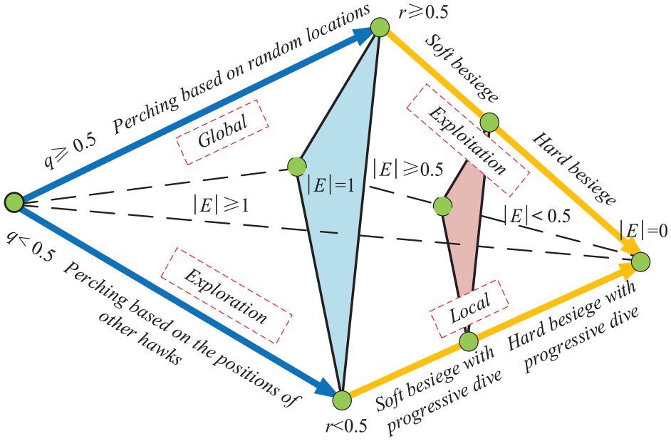
Description of each phase of HHO.
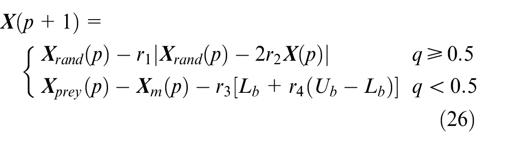
The Harris hawk has two strategies for waiting for finding its prey, which can be modeled as follows:
where
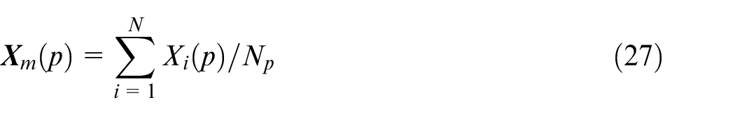
where Xi (p) is the position of each hawk in p iterations, Np is the hawks number. Based on the relationship between prey escape and its energy, the energy of the prey E is simulated as:

Where P is the maximum iterate, and E0 is the initial energy of prey (−1, 1). The Harris hawks attacking strategies process is as follows:
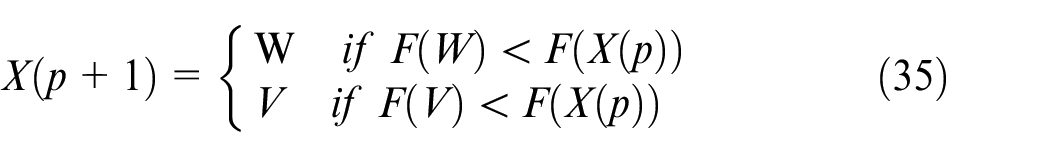
(1) |E| ≥ 0 and r ≥ 0.5 (r is the probability of the prey escaping)
The prey tries to escape, and the hawk positions can be expressed as:
where J = 2(1−r5) represents the prey movement pace during the escape process, and r5∈(0,1).
(2) |E| ≥ 0.5 and r < 0.5
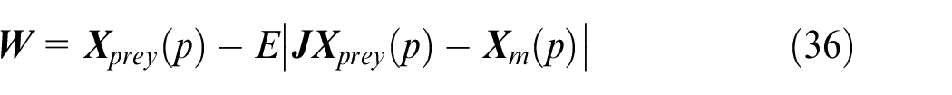
The hawks rapidly dive around the prey several times and determine their position and direction according to the movement of the prey. The position of the hawks can be simulated as follows:


where F(*) is the fitness function, Dp is the search agent space,
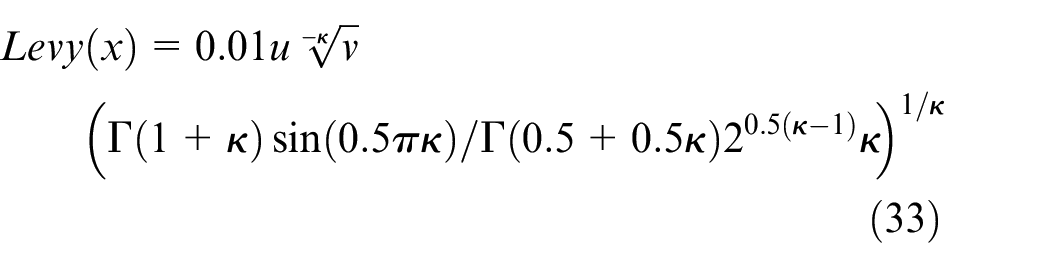
where u, v∈(0,1), and κ = 1.5.
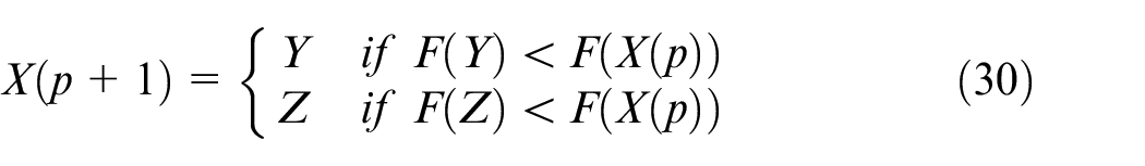
(3) |E| < 0.5 and r >= 0.5
The prey is unable to escape, and the hawk position is updated as follows:

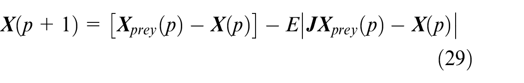
(4) |E| < 0.5 and r < 0.5
Hawks attempt to reduce the distance from the average position of the fleeing prey according to the following rules:

The HHO algorithm removes the derivative part of the limit state function to solve high-dimensional calculation problems more efficiently.
Parameter identification
The HEO model is established by combining the experimental data and the HHO method:
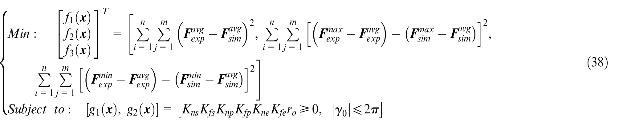
where
The decrease in the objective function is advantageous to find the solution vector conforming to constraints rapidly. 22 This process can be modeled by introducing a penalty function:
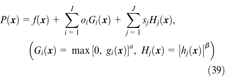
where oi and sj are penalty function coefficients, gi (
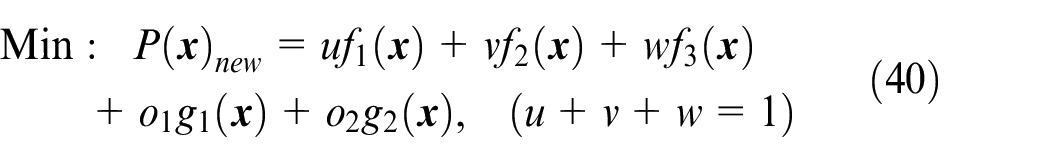
Using the HEO algorithm to calculate the new error function value, the iterative input value is changed according to the feedback value. Once the iterative process is stopped, the parameters can be obtained with the calculating flow shown in Figure 7.
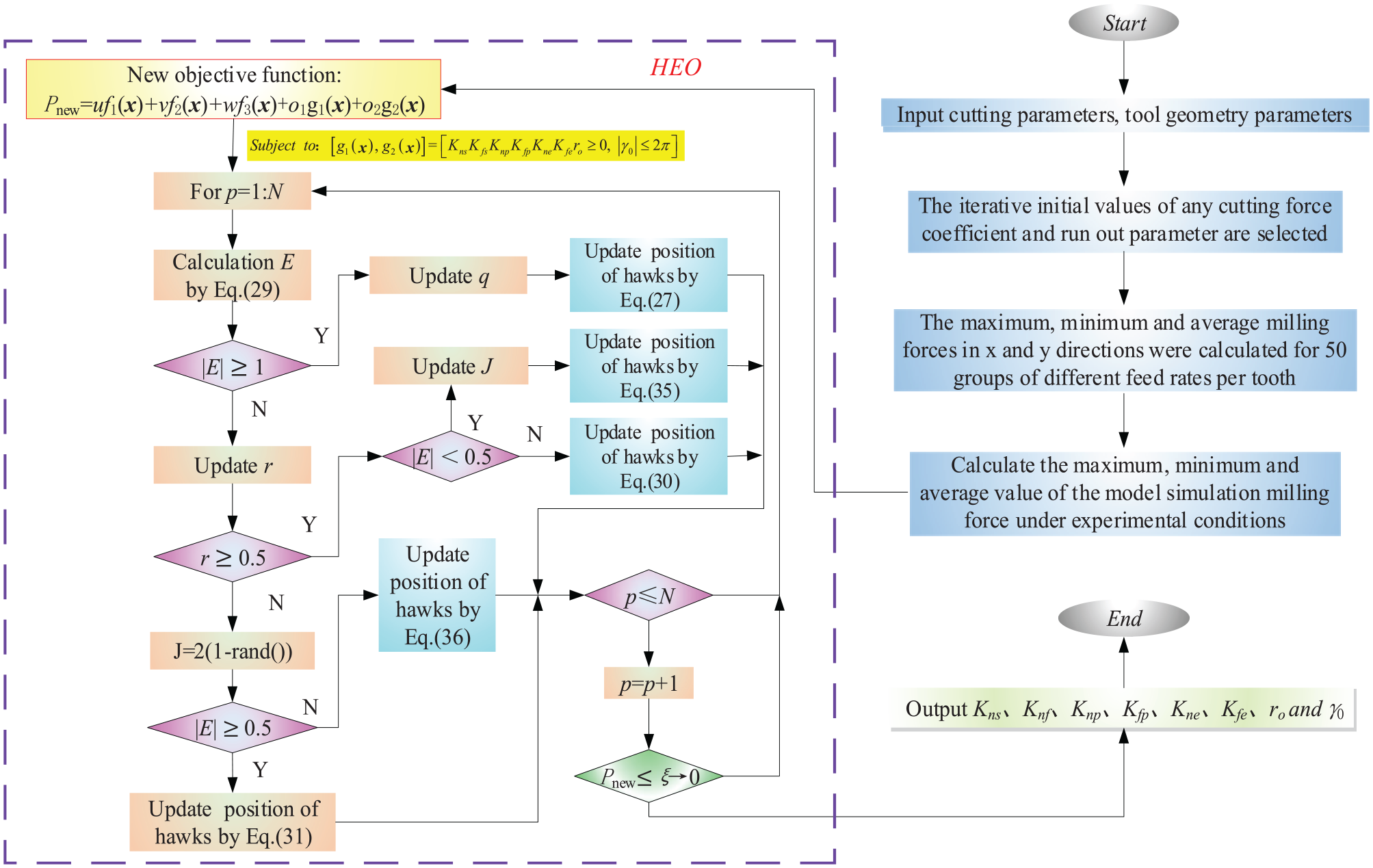
Flow chart of micro-milling parameter identification.
Adaptive Kriging fitting
Adaptive Kriging (AK) is used to fit the established implicit model to save calculation time and facilitate the analysis of extensive sample data. In addition, Monte Carlo Simulation (MCS) 24 method was used to verify the AK-results.
Initial Kriging
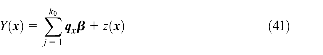
The Kriging method is an improved technology with linear regression analysis, including linear regression and nonparametric parts. 25 The nonparametric part is the realization of the stochastic distribution process, and the Kriging model can be written as:
where
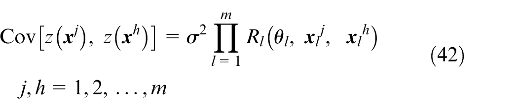
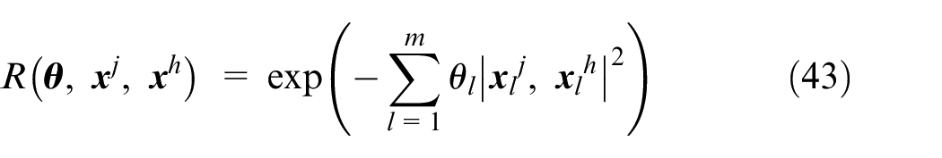
where θl (l=1, 2, …, m) is the correlation parameter, Rl is the correlation function, which is expressed as follows:
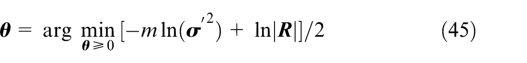
Based on the generalized least squares method, the estimated values of
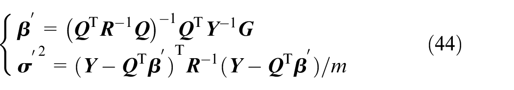
where
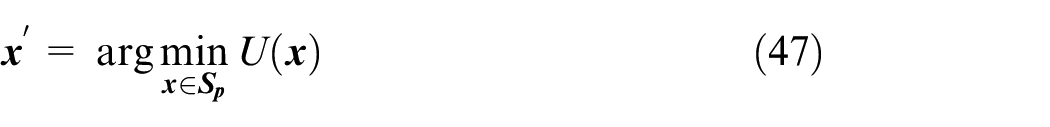
Adaptive-Kriging (AK) method
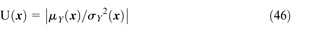
AK method improves the prediction accuracy by analyzing the fault state of the output parameters obtained by the initial Kriging. 26 The model is updated circularly until the adaptive convergence condition is satisfied. The learning process can be outlined as follows:
The Adaptive Kriging update process is as follows:
A sample pool
Samples of N1 input variables from the sample pool
The learning function U(x) corresponding to each sample in the sample pool
When
The complex flexible mechanical model established in Section 2 is fitted by the AK method. Then, many input samples are substituted into the new fitting model for output, providing the basis for the next section – the rapid micro-milling force probability analysis (Figure 8).
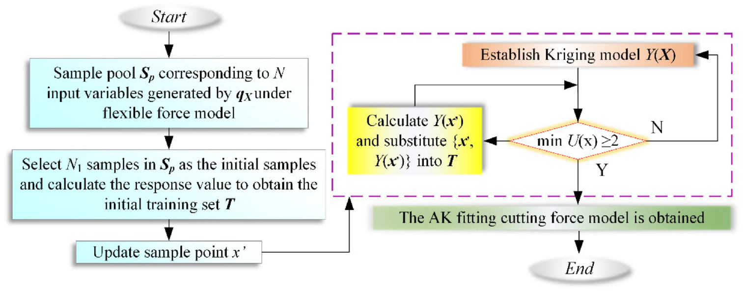
Flow chart of AK method.
Experimental and probability analysis
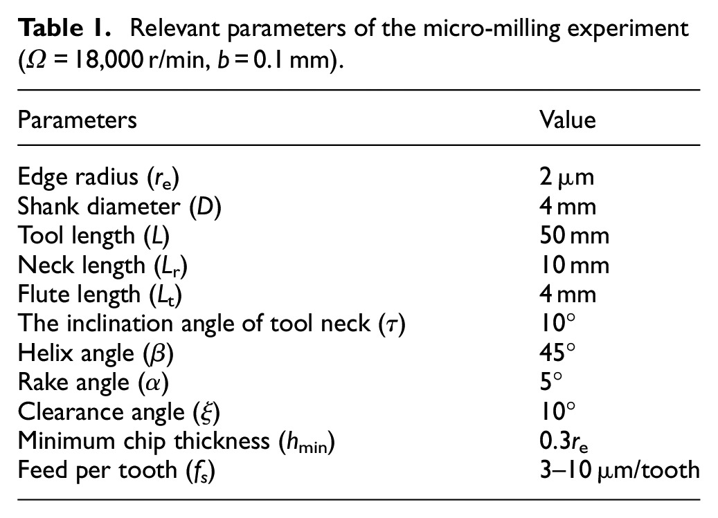
The cutting experiment is carried out on the experimental micro-milling machining center with a maximum electric spindle speed of 24,000 r/min. The workpiece material is Al6061 (90 × 10 × 120 mm), with an elastic recovery rate of 0.1. The micro-milling cutter is a tungsten carbon uncoated two-edged with a diameter of 1 mm. Table 1 outlines the parameters used in the calculation simulation and experimental processes.
Relevant parameters of the micro-milling experiment (Ω = 18,000 r/min, b = 0.1 mm).
As shown in Figure 9, the cutting path is set in the computer control center. The machining coordinate of the machining system is found through the operating handle, and then the cutting command is executed. The force sensor, data collector, and charge amplifier record the force of the micro-milling tool. Finally, the force curve is visualized on the computer, and the data values are obtained.
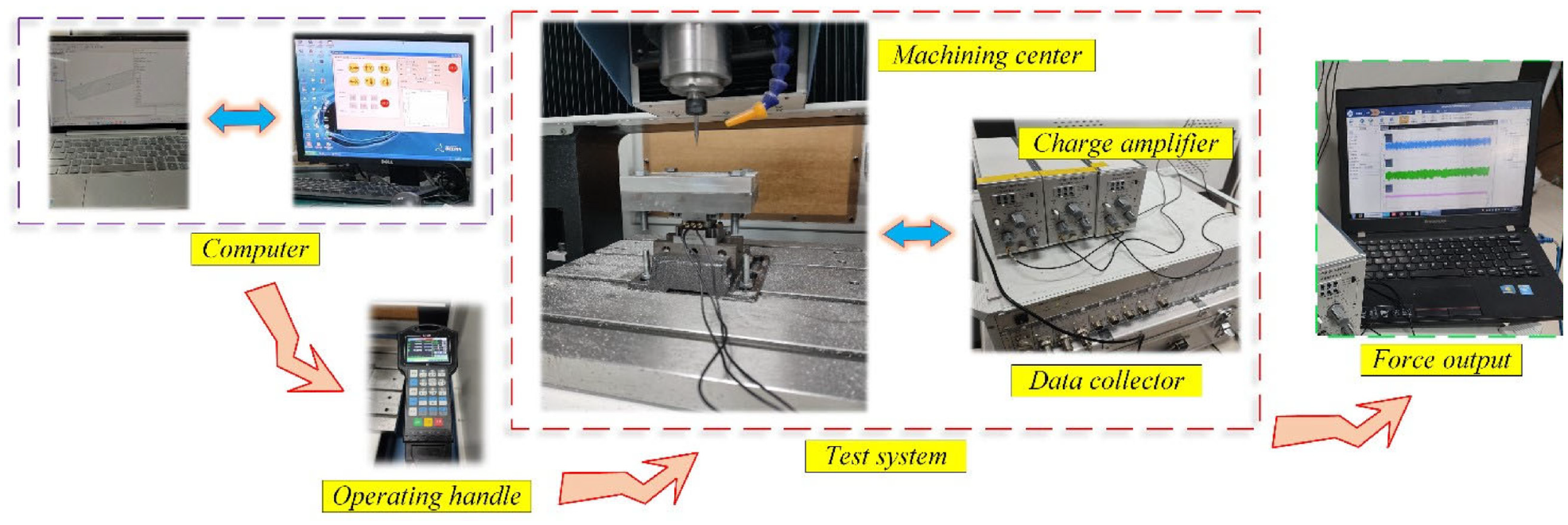
Experimental setup.
Model validation
The parameters obtained using the proposed parameter identification method are listed in Table 2. To verify the output accuracy, the average values of 50 groups of experimental milling force data were obtained and plotted in Figure 10(a).
Cutting coefficient and runout parameters with the minimum error.
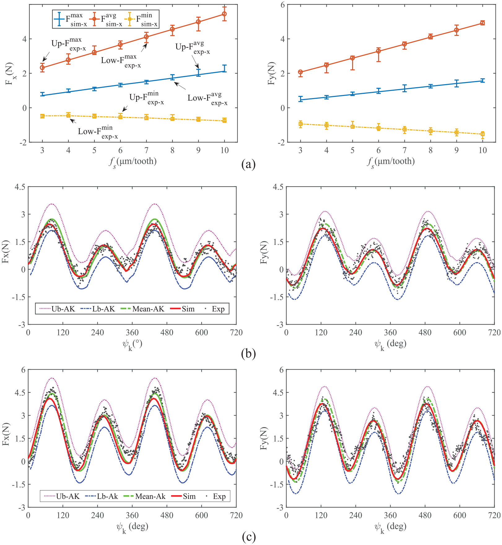
Comparison diagram of cutting force curve: (a) spindle speed 18,000 r/min, cutting depth 100 μm, (b) fs = 4 μm/tooth, and (c) fs = 8 μm/tooth.
As shown in Figure 10(a), the maximum, minimum, and average cutting force values obtained by the flexible milling force model are within the extreme ranges of experimentally-obtained values, with small error values. To further explore the accuracy of the milling force obtained by the established AK method, the cutting forces at the different positions during the milling process are compared and analyzed
The Ub-AK and Lb-AK in Figure 10(b) and (c) represent the extreme-confidence interval range of the superposition effect of the cutting force considering the 95% confidence interval obtained by using the central limit theorem and the big tree law and the error value of AK fitting. Mean-AK is the average value of AK fitting cutting force. Sim and Exp represent the force predicted by the flexible force model and measured experimentally. The results of the comparison are as follows:
The prediction curve agrees with the experimental results, verifying the accuracy of the proposed HEO parameter identification method.
The Mean-AK coincides with the predicted curve of the flexible force model (Sim), indicating that the AK fitting method applies to micro-milling force calculation.
The majority of the experimental data are found in the extreme-confidence interval. A small number of experimental data points are around the boundary, conforming to the nonideal working conditions inherent to the realistic machining process.
Probability characteristic prediction
Following the modeling and analyzing the micro-milling, the probability distribution of the milling force is discussed. In this section, the AK fitting method and the direct MCS method combined with the proposed flexible force model are used to conduct the comparative analysis and determine the accuracy of the result.
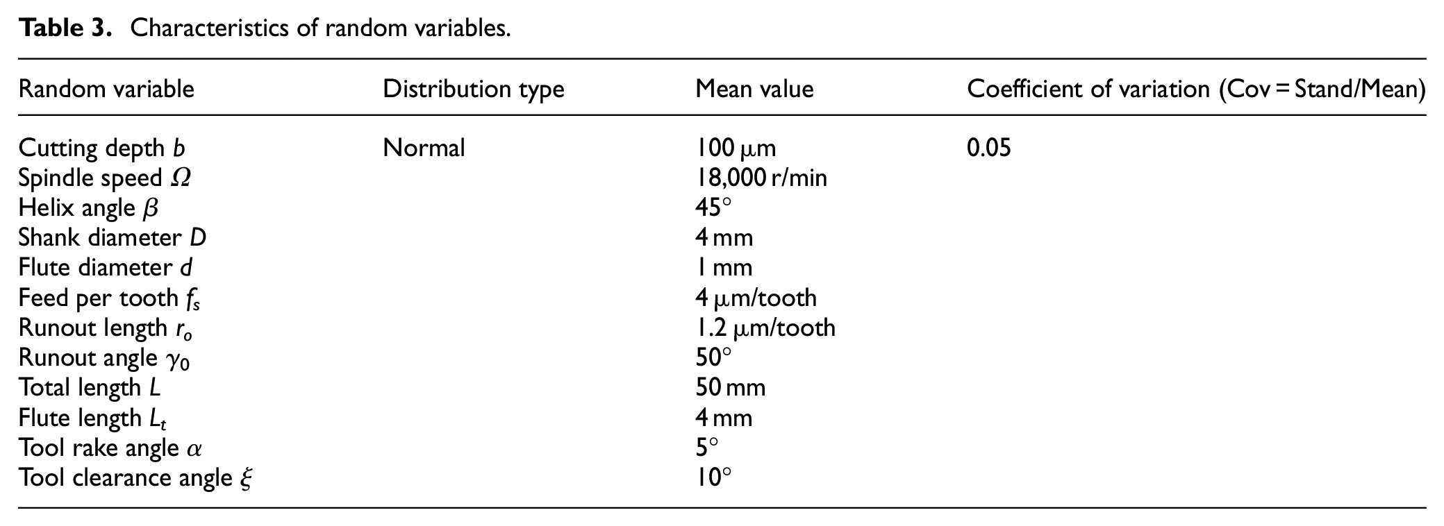
The cutting force at the position angle ψk = 80° was analyzed (100 sample points) to further discuss the differences between the AK and the established models. Based on the characteristic analysis of general machining parameters, 28 the specific distribution of micro-milling parameters can be determined (Table 3). The milling forces are compared, and the corresponding scatters plot obtained using both methods are shown in Figure 11. The curve distribution in the figures shows that the output data obtained by the AK method is practically identical to that obtained by combining the MCS with the proposed flexible force model, which verifies the accuracy of the AK method.
Characteristics of random variables.
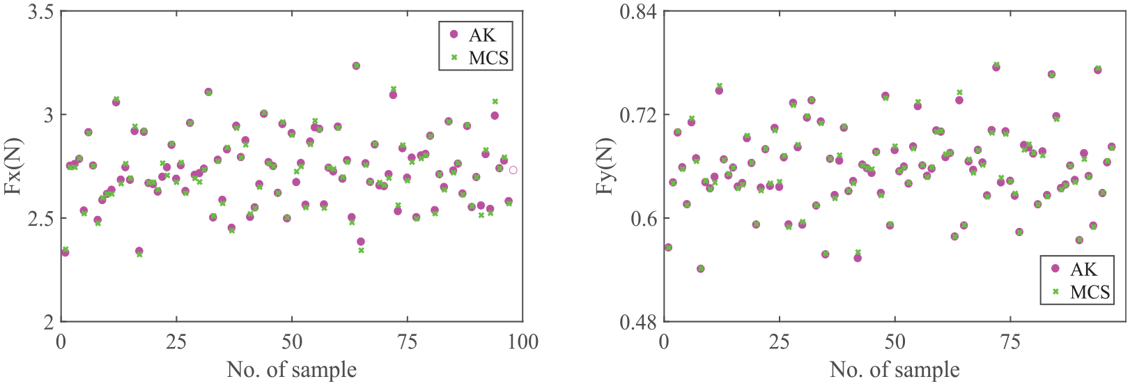
Comparison of scatter plots (ψk = 80°).
Based on the distribution of random parameters in Table 3, each random variable is sampled by the MCS (105) and substituted into the flexible force model and the trained AK model for prediction. Figure 12 shows the probability distribution characteristics of cutting force when position angle ψk = 80°, indicating that the milling force frequencies obtained under the two methods are basically the same. The cutting force distribution is concentrated near the average value with the greater probability value.
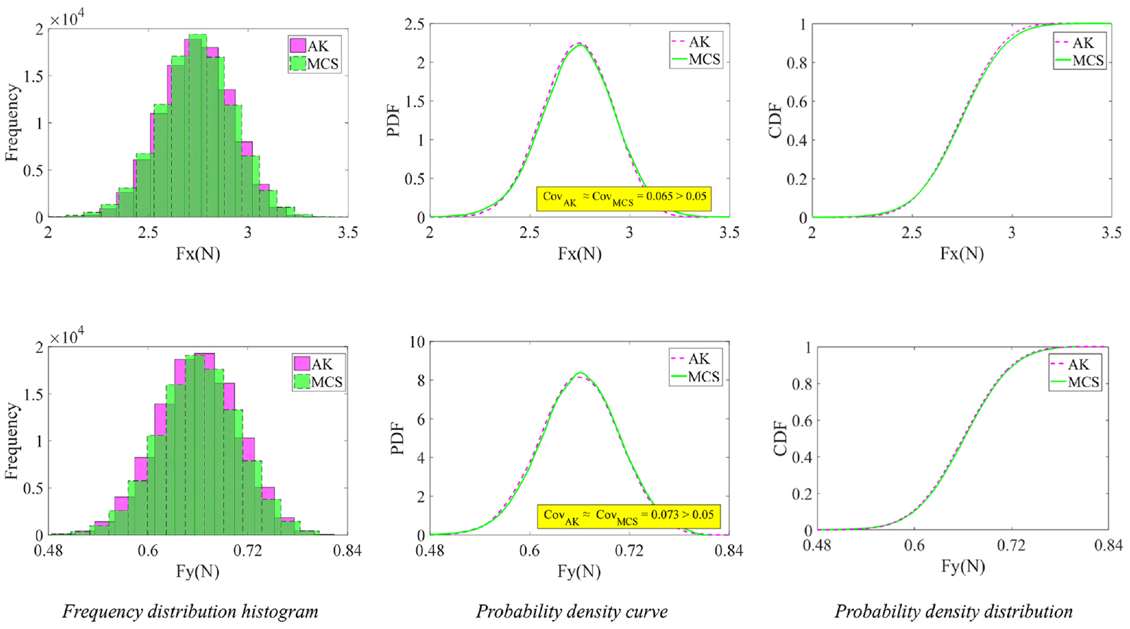
Analysis diagram of cutting force characteristics.
The statistical calculation provided in Figures 10 to 12 shows that the predicted mean value of the cutting force is close to the actual value. Its Cov is greater than the Cov of a single parameter, indicating that the calculation result of the cutting force is unbiased and has strong dispersion. Moreover, the analysis time used by the AK method is 10 min. In comparison, the calculation time used by the flexible force model directly is 240 min, which proves that the analysis of probability problems AK is more efficient.
Conclusion
A new method for identifying the micro-milling parameters using the HEO method is proposed. Based on the identified parameters and cutting mechanism, an accurate flexible cutting force model for micro-milling is established. Combined with the proposed model and AK method, efficient calculation and analysis of cutting force probability characteristics in micro-milling are realized. The main contents of this study can be summarized as follows:
A new micro-milling flexible force model framework is present. The model considers the influences of multiple factors, including the tool runout, IUCT, MCT, material elastic recovery rate, tool deformation and cutting force coupling, and chip separation state. After comparing experimental data and calculation results, it is observed that the proposed mechanical model has a high prediction accuracy.
The HEO parameter identification method for solving the cutting coefficient/parameter of micro-milling is developed. This method integrates the experimental data and mechanical model into the objective optimization function. It directly obtains the coefficients/parameters by using the optimization operation, which overcomes the complexity of repeated experimental measurements.
The AK method is used to reconstruct the functional relationship in the mechanical model, avoiding the time consumption stemming from repeatedly using the complex flexible force model directly. The probability characteristics of micro-milling force are analyzed via AK and direct MCS, respectively.
The curve shown in Figure 10 indicates that the experimental data are distributed within the extreme-confidence interval of cutting force obtained by the AK method, which illustrates that the proposed flexible force model is accurate. The curves in Figures 10 to 12 show that the average values of cutting force simulation is an unbiased estimate of cutting force, and the cutting force has a large dispersion (Cov >0.05), so it is necessary to consider the randomness of parameters when analyzing the cutting force state.
Compared to the traditional mechanical model, this study considers the influence of multiple factors and the uncertainty of processing parameters on the micro-milling force modeling. As such, it is more in line with the actual engineering situation. The actual distribution of parameters can be used as a research issue in the forthcoming studies. The above research results have positive guiding value for analyzing the precise micro-milling mechanism, improving machining quality, and enhancing manufacturing efficiency.
Footnotes
Declaration of conflicting interests
The author(s) declared no potential conflicts of interest with respect to the research, authorship, and/or publication of this article.
Funding
The author(s) disclosed receipt of the following financial support for the research, authorship, and/or publication of this article: The authors gratefully acknowledge the support of the National Natural Science Foundation of China (51975110), Liaoning Revitalization Talents Program (XLYC1907171), and Fundamental Research Funds for the Central Universities (N2003005, N2203004), Key-Area Research and Development Program of Guangdong Province (2020B090928001).