Sage Journals: Discover world-class research

Abstract

The anisotropy and nonuniformity of wood-plastic composites (WPCs) affect the milling tool, which rapidly wears during high-speed milling of WPCs. Thus, the evolution mechanism of tool failure becomes complicated, and the prediction of tool wear cannot be precisely described mathematically. A neural network based on tool wear test was proposed to predict the tool wear condition during high-speed milling of WPCs. The traditional backpropagation (BP) neural network easily falls into the local optimal solution. A genetic algorithm (GA-BP) neural network prediction model was established by using the GA to optimise its initial weight and threshold. The BP model and the GA-BP model were evaluated in terms of mean square error and training times, and the generalisation verification was applied to the prediction model. After analysing and comparing the results of the two models, the GA-BP neural network model has better training speed and accuracy under the test conditions. The relative error between the predicted value and the actual value is controlled within 5%.

Keywords

Tool wear wood-plastic composite (WPC)high-speed milling neural network prediction model

Introduction

With the growing shortage of natural wood resources, some artificial wood panels are gradually accepted and used by consumers. Among them, wood-plastic composites (WPCs) are preferred by many industries due to their dual properties, which are natural plant fibre and thermoplastic polymer materials. They are applied in green buildings, agricultural machinery and interior design. Although WPCs can be moulded once by extrusion or injection, performing secondary processing is necessary on products with complex profiles, dimensions and assembly requirements. In high-speed milling of WPCs, the degree of tool wear is crucial, and the use of severely worn tool reduces machining efficiency and product quality, and remarkably increases the energy consumption of the machine.¹ Hence, the use of selected cutting parameters to predict tool wear is an effective means to save time and reduce machining cost in processing WPCs.

Backpropagation neural network (BPNN) is a multilayer feedforward neural network trained in accordance with the error BP algorithm. This algorithm has the processing ability of parallel distributed information and is suitable for applications in prediction, classification and diagnosis.^2,3 Singh et al.⁴ pointed out that BPNN can effectively learn the wear law of the tool and can be used in the actual tool wear prediction. Many scholars have investigated the relationship between cutting factors and tool wear. Fan et al.⁵ selected the cutting speed, feed rate and cutting depth as input variables and the flank wear VB as the output variable to establish a BPNN prediction model of tool wear. The results show that an effective prediction interval is found for predicting tool wear by BPNN. When the cutting speed is near the training sample data, the relative error between the prediction value and the experimental result of tool wear can be controlled within 10%. Gao et al.⁶ predicted the flank wear of single-tooth BTA tools by BPNN. The experimental and simulation results show that BPNN has good generalisation ability for predicting tool wear. Quiza et al.⁷ established a neural network of multilayer perceptron type to predict the flank wear for several cutting parameters in hardened D2 (AISI) steel turning. The neural network allows more accurate predictions for the tool wear to be obtained. This condition is shown by comparing the obtained neural network with statistical multiple regression. Paul and Varadarajan⁸ established regression model and BPNN model to predict tool flank wear and found that the model based on artificial neural network (ANN) is better than the regression model in predicting tool wear. Özel and Karpat⁹ utilised trained neural network models to predict the surface roughness and flank wear for various cutting conditions. The developed prediction system is found to be capable of accurate surface roughness and tool wear prediction for the range it has been trained. The neural network models are compared with the regression models. The neural network models provide better prediction capabilities because they generally offer the ability to model more complex nonlinearities and interactions than linear and exponential regression models. Comparing statistical regression with neural networks, Mukherjee and Ray¹⁰ pointed out that although statistical regression may work well for modelling, this technique may not describe precisely the underlying nonlinear complex relationship between the decision variables and responses.

A series of neural network and artificial intelligence -based methodologies have been developed and applied to the prediction of tool wear. Considering the complexity of wear status classification, Khajavi et al.¹¹ used a multilayer neural network and selected the root mean square of the motor current, feed, cutting depth and tool speed as the input of the model and the flank wear as the output. The results show that the designed tool wear monitoring system has good performance. Chen et al.¹² applied a deep belief network (DBN) to predict tool flank wear and confirmed the superiority of DBN in predicting tool wear. Tang et al.¹³ applied a convolutional neural network with deep residual network structure to the prediction of milling tool wear and obtained high prediction accuracy. Srikant et al.¹⁴ used simulated annealing algorithm to effectively optimise the structure of neural network. The outcomes reveal that the prediction error is remarkably reduced. Xue et al.¹⁵ used particle swarm optimisation (PSO) to optimise BPNN. The results show that the PSO-BP model has better convergence and higher universality than the BP model, and its performance is obviously better than BPNN. Scheffer et al.¹⁶ conducted a comparative evaluation with ANNs and hidden Markov models (HMMs) for modelling complex correlations between the input set of sensor signal functions and tool life during turning. Ojha and Dixit¹⁷ assessed tool wear by fitting a best fit line on the data in the steady wear zone and establishing the time until tool failure by extrapolation. ANNs are often used to predict lower, upper and estimates of tool life. The neural network developed by feedforward BP algorithm is one of the current trends.¹⁸ Balazinski et al.¹⁹ used feedforward BPNNs, fuzzy decision support systems and neural network-based fuzzy inference systems as artificial intelligence methods to estimate turning tool wear. The practicability of the three methods is compared. Although the average prediction error of the neural network is acceptable, the training time is long and is inconvenient in practical applications.

Although BPNN has unique advantages in dealing with multifactor, uncertain and nonlinear problems of tool wear prediction, the traditional BPNN is prone to local optimal solution and slow convergence.^20,21 Genetic algorithm (GA) is a computer-based search algorithm that is suitable for optimising various functions.^22,23 As another branch of intelligent control in the search process, GA can overcome the shortcomings of slow convergence and easy to fall into local optimal solution. GA can optimise the weight and threshold of BPNN, extend the search space of neural network system and improve computational efficiency.^24–26 Bi et al.²⁷ obtained a 1D prediction model of tool volume wear by using an improved GA-BP algorithm and realised the accurate prediction of tool wear under small sample conditions. Kaya et al.²⁸ established a tool wear monitoring system based on support vector machine and GA. This system is particularly useful in identifying sharp tools.

This study aimed to investigate tool wear machining problems. The tool wear test in high-speed milling of WPCs was conducted by using central composite design method. On the basis of the test data, the BPNN model optimised by GA was established by using mathematical software MATLAB. The established model was applied to the tool wear prediction in high-speed milling of WPCs, thereby providing the theoretical basis for selecting reasonable processing parameters and timely replacement of tools.

Mathematical model of BPNN and GA

Mathematical model of BPNN

BPNN is a multilayer feedforward neural network trained based on error BP algorithm. Its model topology consists of input layer, hidden layer and output layer. The graph below (Figure 1) shows the structure of a BPNN with one hidden layer.

Figure 1.

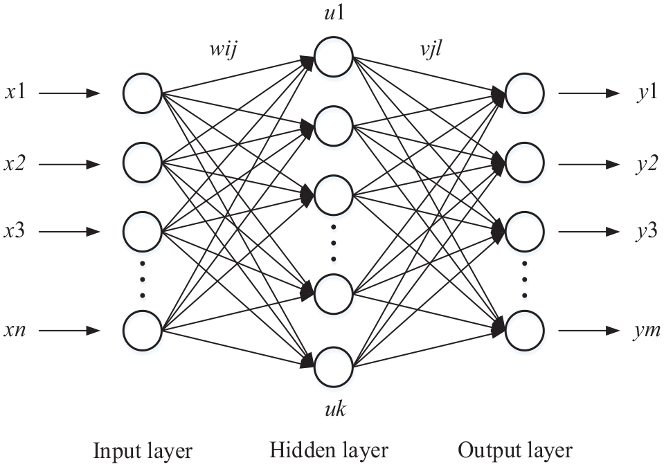
Architecture diagram of three-layer BPNN.

The input variables are x₁, x₂, x₃⋯, x_n, the hidden layer variables are u₁, u₂, u₃⋯, u_k, the output variables are y₁, y₂, y₃, ⋯, y_m, the actual output variables (target output) are T = t₁, t₂, t₃, ⋯, t_m, the connection weight between the input layer and hidden layer is w_ij, the threshold is θ_j, the connection weight between the hidden layer and output layer is v_jl, and the threshold is θ_l (i = 1, 2, 3, ⋯, n; j = 1, 2, 3, ⋯, k; l = 1, 2, 3, ⋯, m).

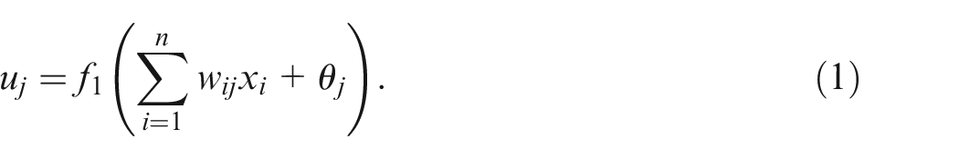
When the input signal is propagating in the forward direction, the output of the jth node in the hidden layer is

u_{j} = f_{1} (\sum_{i = 1}^{n} w_{ij} x_{i} + θ_{j}) .

(1)

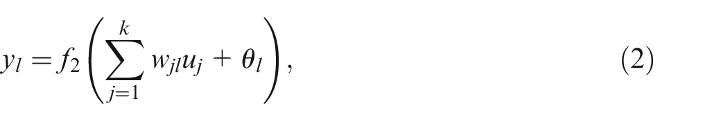
The output of the lth node in the output layer is

y_{l} = f_{2} (\sum_{j = 1}^{k} w_{jl} u_{j} + θ_{l}),

(2)

where f(x) is a transfer function and used as Sigmoid function.¹⁹f(x) is continuously differentiable, and

f^{'} (x) = f (x) [1 - f (x)] .

(3)

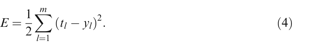
In case of error BP, when the output is inconsistent with the target output, an error E is found, which is set as

E = \frac{1}{2} \sum_{l = 1}^{m} {(t_{l} - y_{l})}^{2} .

(4)

In network training, the weights and thresholds are adjusted continuously to reduce the network error to the preset minimum or to stop the maximum training times. The prediction samples are inputted to the trained network to obtain the prediction results.

Mathematical model of GA-BPNN

GA is an adaptive global optimisation probability search algorithm that simulates the genetic and evolutionary processes of living things in the natural environment. GA is based on Darwin’s law of natural selection. Selecting the key parameters of GA, such as population size, number of generations, crossover rate and mutation rate, carefully is extremely important.^29,30 This algorithm regards all individuals in the population as research objects and achieves a stable, optimal breeding and selection process through the hybridisation and variation of individual genes, until the population puts forward the best solution.³¹ Compared with traditional algorithms, GAs use global optimisation rather than point-to-point search, making it easier to achieve global optimality.

The method of using GA to optimise BPNN can achieve complementary advantages, improve convergence speed and obtain optimal solution faster. Firstly, the GA is used to optimise the initial weights and thresholds of the network to find the optimal initial weights and thresholds. The optimal initial weights and thresholds are then assigned to the BPNN. Finally, the BP algorithm is used to find the optimal solution in small space. The execution process of BPNN optimised by GA is shown in Figure 2.

Figure 2.

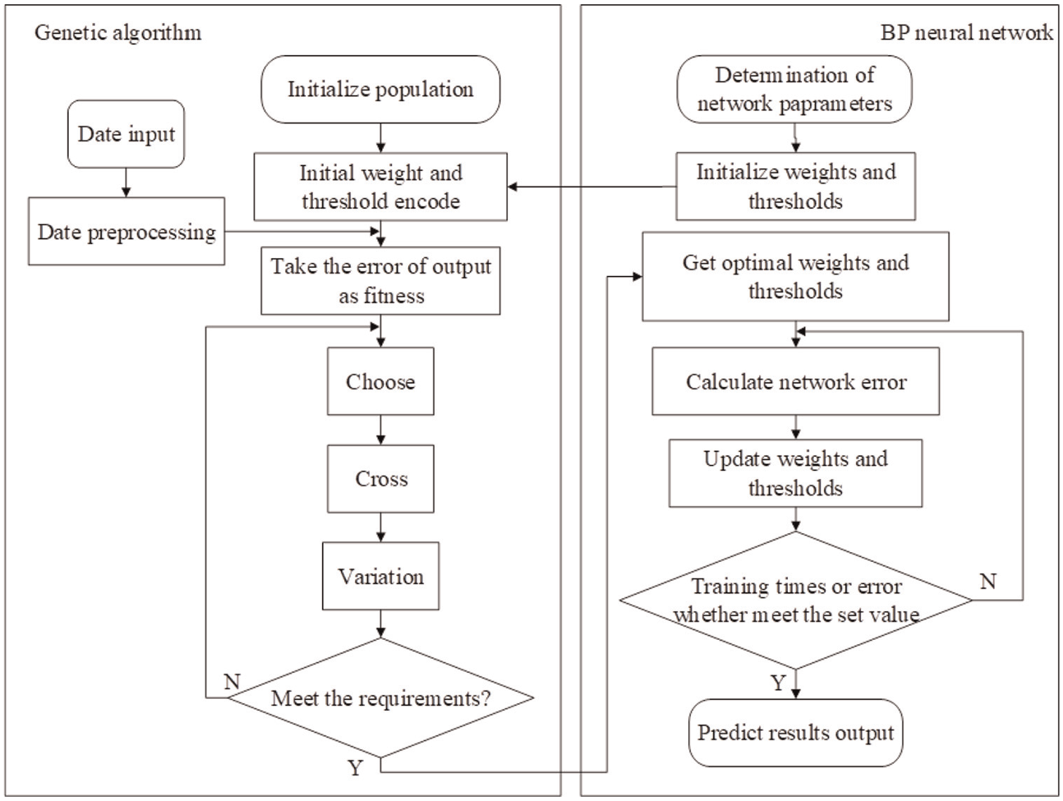
Flow chart of BPNN optimised by GA.

In this study, the absolute value of the error between the network prediction output and the target output was taken as the fitness function of the GA. The calculation formula is shown in equation (5).

F = k (\sum_{i = 1}^{n} abs (y_{i} - o_{i})),

(5)

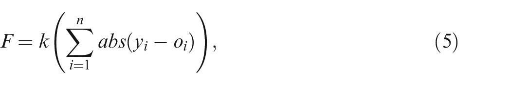
where n is the total number of network output nodes, y_i is the target output, o_i is the prediction output and k is the coefficient.

In this study, roulette method is used in the selection process to ensure the inclusion of individuals with low fitness. The formula is shown below

f_{i} = k / F_{i}, P_{i} = f_{i} / \sum_{i = 1}^{N} f_{i},

(6)

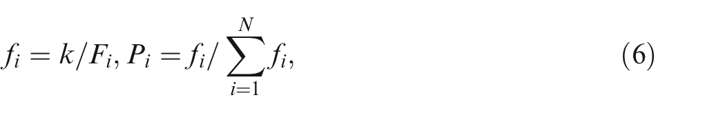
where k is the coefficient, and F_i is the fitness value of individual i. The smaller the fitness value, the better the result. Thus, the reciprocal of fitness value is found before individual selection. N is the total number.

In the crossover step, two chromosomes are randomly selected, and one or more positions in the chromosome are selected for exchange. The calculation formula is shown in equation (7).

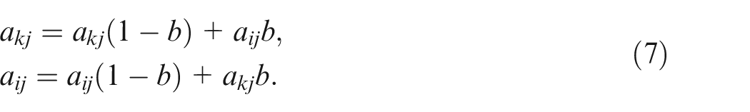
\begin{matrix} a_{kj} = a_{kj} (1 - b) + a_{ij} b, \\ a_{ij} = a_{ij} (1 - b) + a_{kj} b . \end{matrix}

(7)

The formula indicates that the kth chromosome, a_k and the ith chromosome, a_i intersect at the j position; b is a random number between 0 and 1.

In the mutation step, the jth gene of the ith individual is selected for the mutation operation, which is calculated by using equation (8).

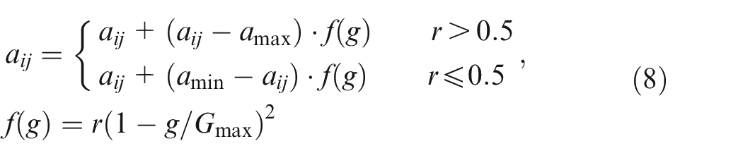
\begin{matrix} a_{ij} = {\begin{matrix} a_{ij} + (a_{ij} - a_{max}) \cdot f (g) r > 0.5 \\ a_{ij} + (a_{min} - a_{ij}) \cdot f (g) r \leq 0.5 \end{matrix}, \\ f (g) = r (1 - g / G_{max})^{2} \end{matrix}

(8)

where a_max and a_min are the upper and lower bounds of gene a_ij, respectively, g is the current iteration number, G_max is the maximum number of evolutions and r is a random number between 0 and 1.

Experiment of tool wear

Experiment preparation

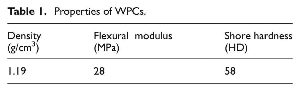
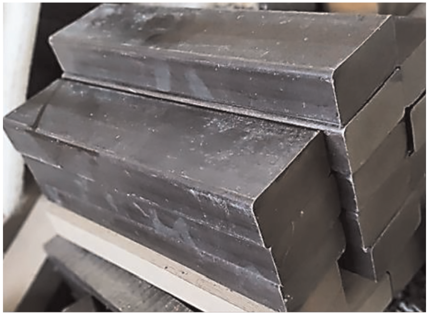
The sample used in the test is wood flour/polyethylene composite material, which is a type of WPC material and has good water resistance and corrosion resistance. The sample size is 322 mm (L), 80 mm (W) and 40 mm (H), as shown in Figure 3. The material is composed of 50% wood flour, 25% polyethylene and 25% adhesive, with a density of 1.19 g/cm³. The general characteristics of the material are shown in Table 1.

Table 1.

Properties of WPCs.

Density(g/cm³)	Flexural modulus(MPa)	Shore hardness(HD)
1.19	28	58

Figure 3.

Test samples.

The tool nose width (NW) is used as the characteristic value of tool wear in this test, as shown in Figure 4, and the standard for blunt NW = 0.5 mm. Ultrasonic cleaning was performed on each set of blades to eliminate surface attachments after the test.

Figure 4.

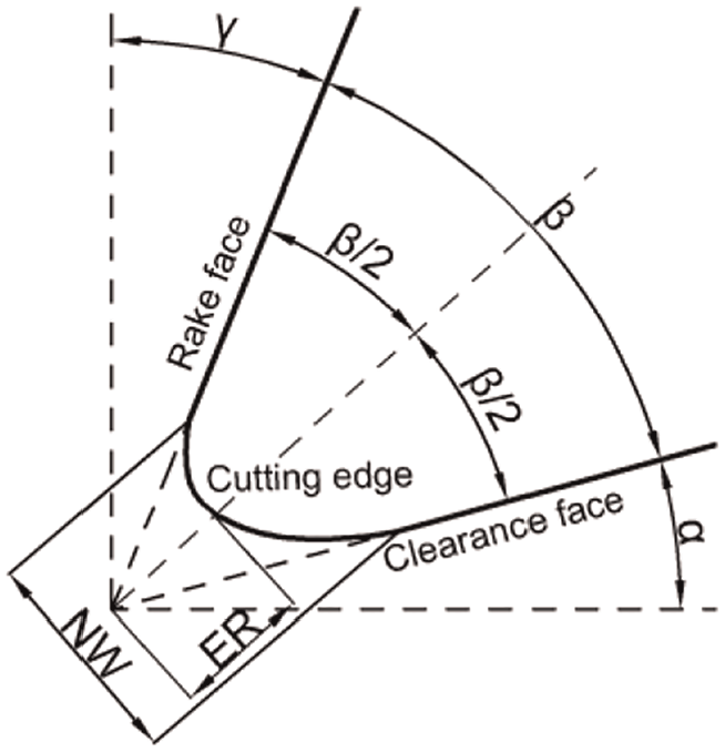
Angular and microgeometrical parameters of the cutting tool.

The tool NW was measured with a Nikon ds-u3ds digital microscopic imaging system, as shown in Figure 5. Figure 6 shows a measurement diagram of tool wear under a microscope.

Figure 5.

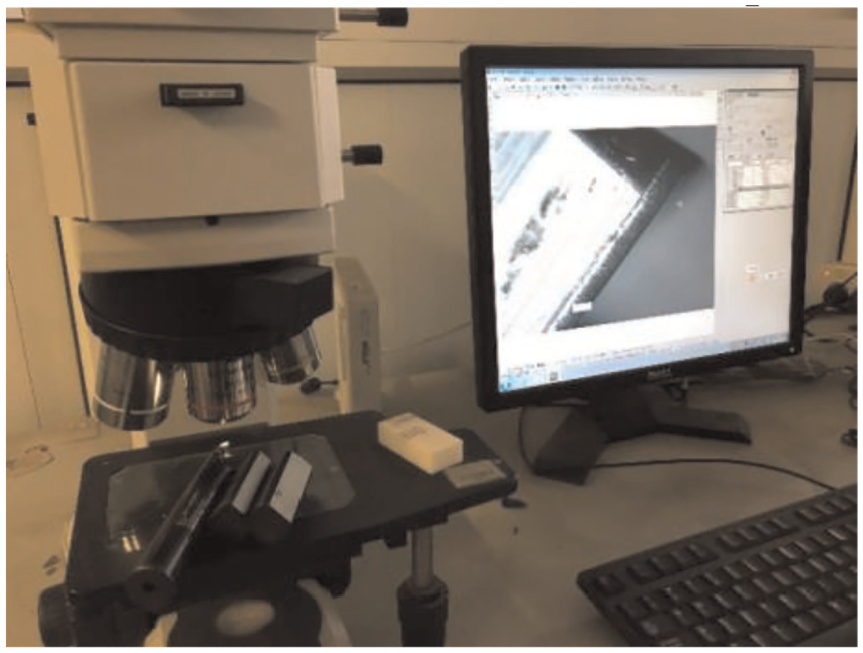
Nikon DS-U3 DS digital microimaging system.

Figure 6.

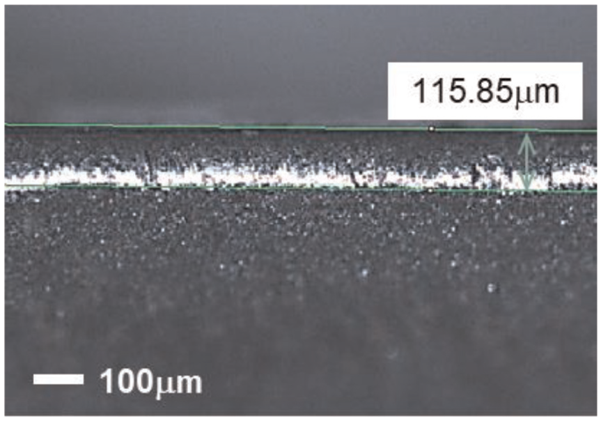
Measurement of tool NW under the microscope.

Experimental equipment

The equipment used in the test is a five-axis machining centre produced by MIKRON, Switzerland, with a maximum spindle speed of 20,000 rpm, as shown in Figure 7. In addition to the basic drilling, milling, boring, tapping and other processing methods, the equipment is furnished with a laser tool setter and a workpiece probe, which can realise the dynamic detection of the tool and the workpiece. This feature results in a significant improvement on the machining accuracy. Figure 8 shows the workpiece clamping diagram during actual machining.

Figure 7.

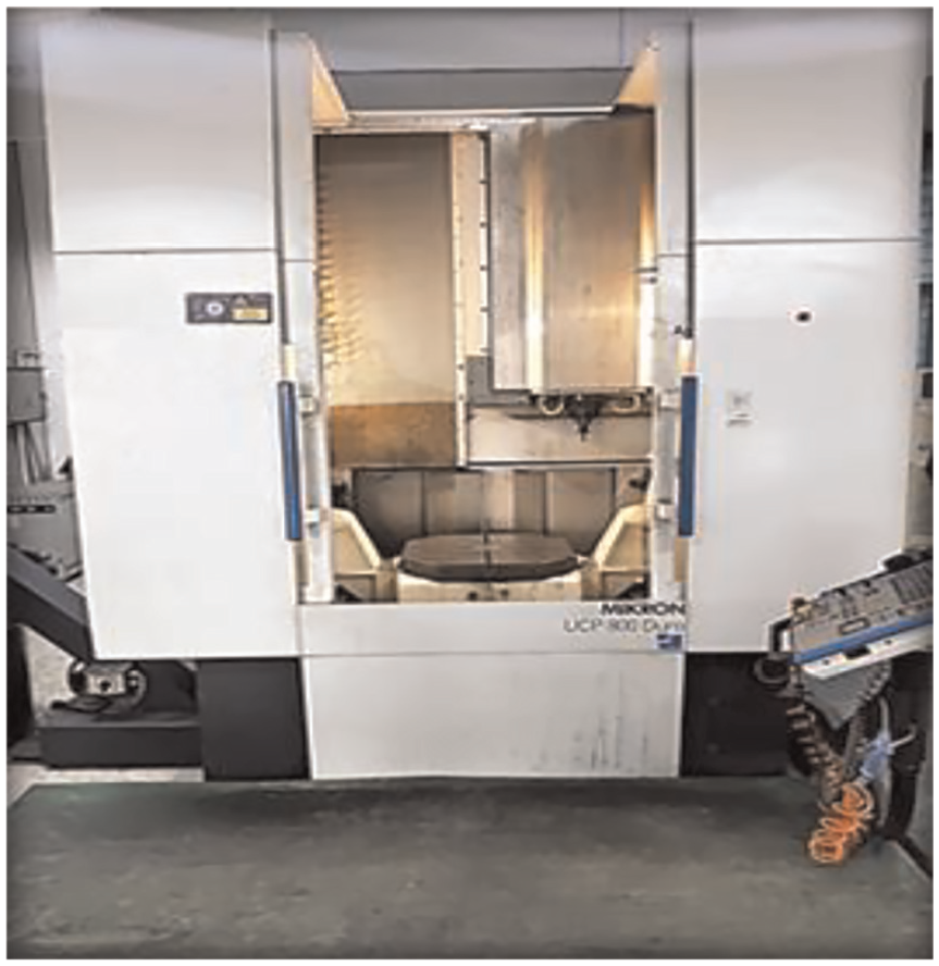
UCP 800 Duro CNC machining centre.

Figure 8.

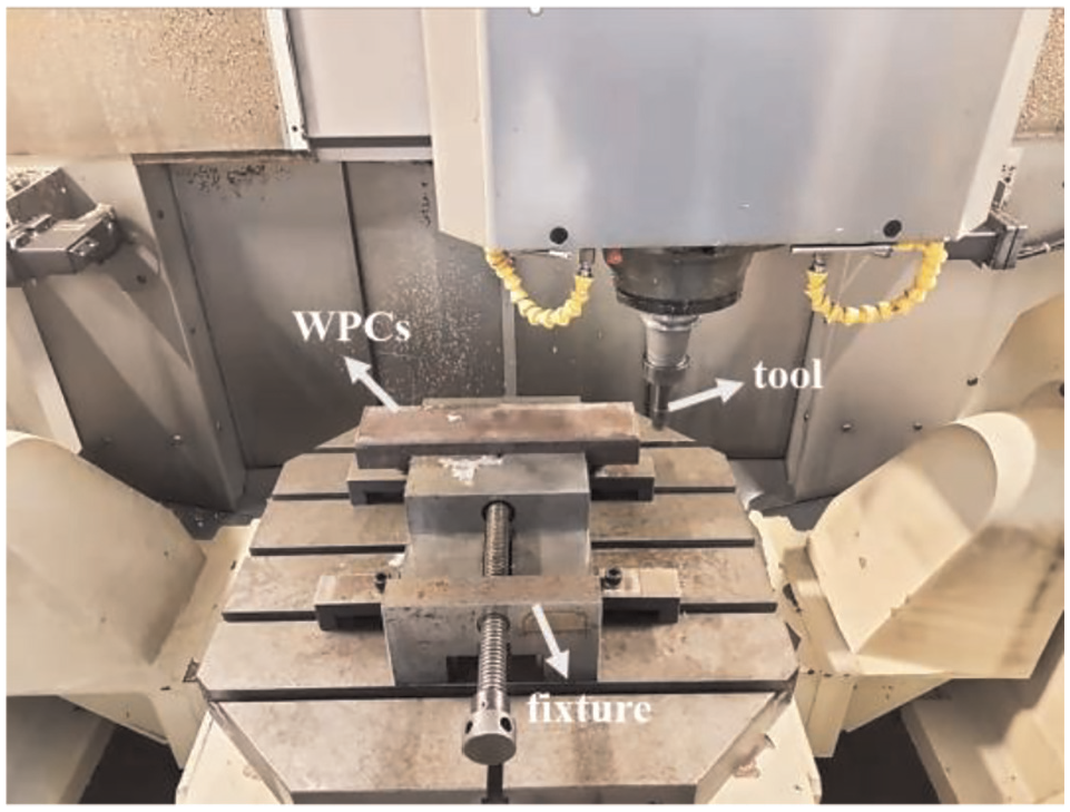
Material clamping diagram of WPCs.

Experimental tool

The uncoated cemented carbide inserts produced by Zhuzhou Diamond Cutting Co., Ltd. (Zhuzhou, China) were used in the test. The geometrical parameters and specifications of the inserts are shown in Table 2 and Figure 9, respectively. At the beginning of the test, the abovementioned blades were installed on a 20 mm diameter cutter arbour, and its model number was EMP01-020-G20-AP11-02 (Figure 10).

Table 2.

Specification parameters of the blade.

Bladetype	Size: L $\times$ I.W $\times$ S (mm)	Rake angle $γ_{0}$ ( $°$ )	Reliefangle $α_{0}$ (°)	Cornerradiusr (mm)
YD201	12.24 $\times$ 6.5 $\times$ 3.6	19	11	0.4

Figure 9.

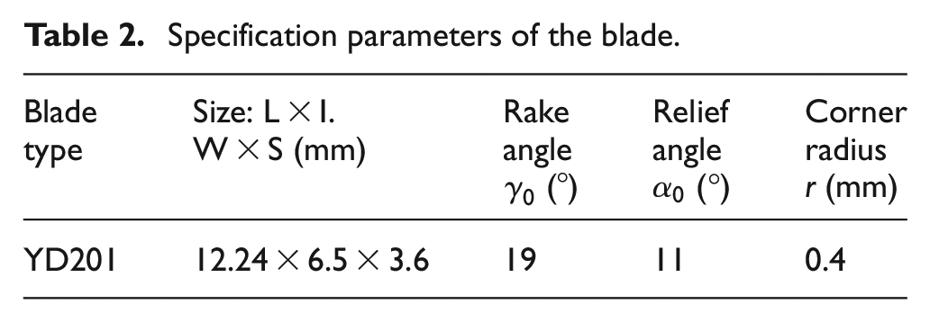
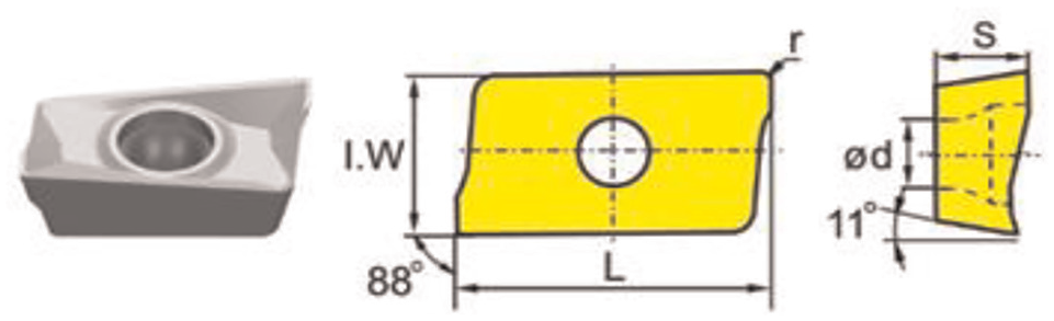
Diagram of blade geometry parameters.

Figure 10.

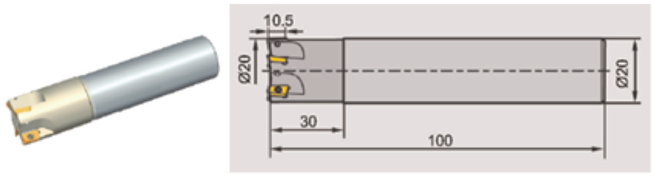
Diagram of cutter arbour geometry parameters.

Experimental results of tool wear

A comprehensive experiment was conducted to record the relationship between tool wear and cutting parameters and establish a GA-BPNN prediction model. The carbide tool was adopted to conduct the high-speed milling tool wear test of WPCs. The tool NW was used to represent the wear of the tool.

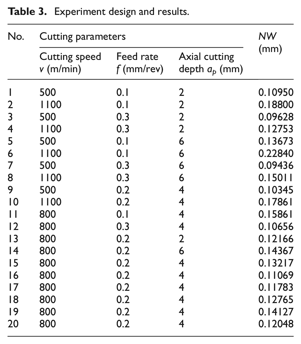
Single factor method was used for the experimental design. Reverse milling method was adopted. The radial depth of cut was 5 mm, and the milling length of each group was 21.12 m. The face-centred CCD (CCF) in the response surface method was selected for the experimental design. In the experiment, cutting speed, feed rate and axial cutting depth were selected for the test design of three factors and three levels.³² This design requires 20 sets of tests, which include 8 sets of factor designs, 6 sets of centre point designs, and 6 sets of axial point designs. The experiment’s design and results are shown in Table 3.

Table 3.

Experiment design and results.

No.	Cutting parameters			NW(mm)
No.	Cutting speedv (m/min)	Feed ratef (mm/rev)	Axial cuttingdepth a_p (mm)	NW(mm)
1	500	0.1	2	0.10950
2	1100	0.1	2	0.18800
3	500	0.3	2	0.09628
4	1100	0.3	2	0.12753
5	500	0.1	6	0.13673
6	1100	0.1	6	0.22840
7	500	0.3	6	0.09436
8	1100	0.3	6	0.15011
9	500	0.2	4	0.10345
10	1100	0.2	4	0.17861
11	800	0.1	4	0.15861
12	800	0.3	4	0.10656
13	800	0.2	2	0.12166
14	800	0.2	6	0.14367
15	800	0.2	4	0.13217
16	800	0.2	4	0.11069
17	800	0.2	4	0.11783
18	800	0.2	4	0.12765
19	800	0.2	4	0.14127
20	800	0.2	4	0.12048

Tool wear prediction model basedon GA-BPNN

Making a reasonable selection of the model parameters, including BPNN parameters and GA parameters, is necessary before using the GA-BPNN to construct the tool wear prediction model.

Parameter setting of BPNN

BPNN includes structure parameters (the number of network layers and nodes) and structure function (transfer function, training function).

Network structure parameters

Considering the generalisation ability of neural network, the 3-1-1 structure of neural network is selected in this study. Three major factors affect NW in processing: the cutting speed, feed rate and axial cutting depth. Thus, the number of input layer nodes is 3. The number of output layers is 1, which corresponds to NW. Proper selection of the number of neurons and activation function in the hidden layers significantly affect the effectiveness of predicting the value of tool wear.²⁷ If the number of hidden layer nodes is extremely large, then the training time of the model will be extremely long, and the error will be large. Conversely, if the number of hidden layer nodes is extremely small, then the generalisation ability and fault tolerance of the model will be reduced. Currently, no theories and methods are established to determine the optimal number of hidden layer nodes, which are commonly determined by empirical equation (9) and trial algorithm.³³ In accordance with equation (9), the number of hidden layer nodes ranges from 1 to 12. After extensive testing, the model has the best prediction ability when the number of nodes in the hidden layer is 1. Hence, the number of nodes in the hidden layer is determined to be 1.

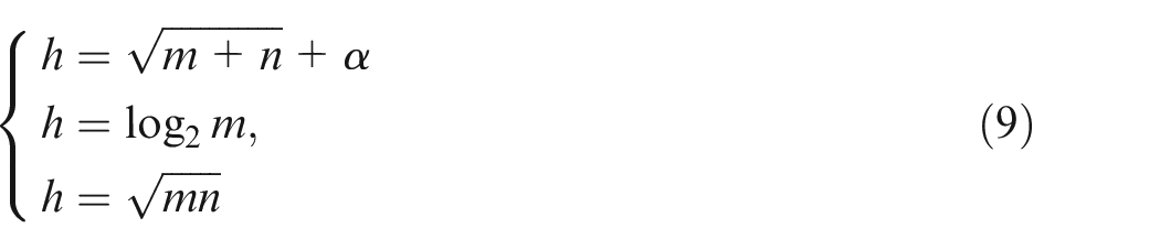
{\begin{matrix} h = \sqrt{m + n} + α \\ h = \log_{2} m \\ h = \sqrt{m n} \end{matrix},

(9)

where h is the number of hidden layer nodes, m is the number of input layer nodes, n is the number of output layer nodes, and α is a constant between 1 and 10.

Network structure function

The tansig function was selected as the transfer function of hidden layer, the purelin function as the transfer function of output layer and trainlm function as the network training function³⁴ by analysing the mapping relationship between input (cutting parameters) and output (NW).

After determining the network parameters, the GA-BPNN structure model is shown in Figure 11, and the corresponding parameters are shown in Table 4.

Table 4.

Structure model parameters of BPNN.

Nodes ofinput layer	Nodes ofoutput layer	Number of hidden layers	Nodes ofhidden layer	Transfer function		Training function
Nodes ofinput layer	Nodes ofoutput layer	Number of hidden layers	Nodes ofhidden layer	Hidden layer	Output layer	Training function
3	1	1	1	tansig	purelin	trainlm

Figure 11.

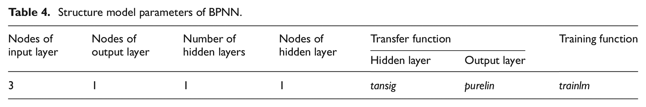
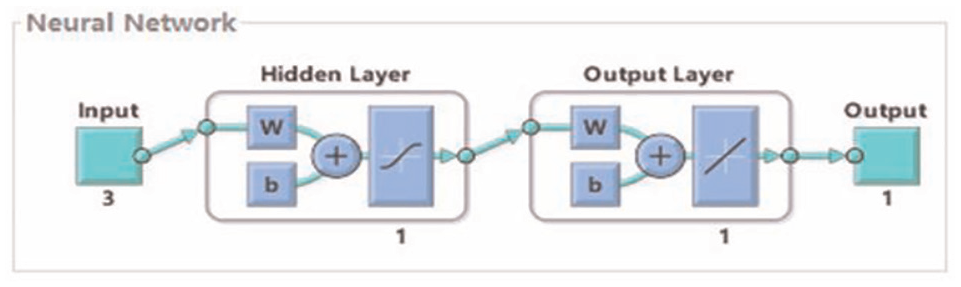
Structure model of GA-BPNN (w – weight,b – threshold).

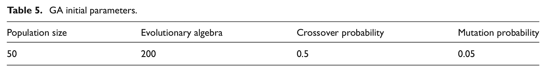
In the above figure, the number of neurons in the input layer is 3: the cutting speed, feed rate and axial cutting depth. The transfer function of the hidden layer is tansig, and the number of neurons is 1. In accordance with equation (1), the output of the neurons in the hidden layer is $u_{1} = tansig (w_{1} * x + b_{1})$ . A neuron (NW) is found in the output layer, and the transfer function is purein. In accordance with equation (2), the output of the neuron of the output layer is $y_{2} = purelin (w_{2} * u_{1} + b_{2})$ .

Parameter setting of GA

The parameters of GA include population, evolutionary algebra, crossover probability and mutation probability. The corresponding parameters are shown in Table 5.

Table 5.

GA initial parameters.

Population size	Evolutionary algebra	Crossover probability	Mutation probability
50	200	0.5	0.05

Results and discussion

Network training

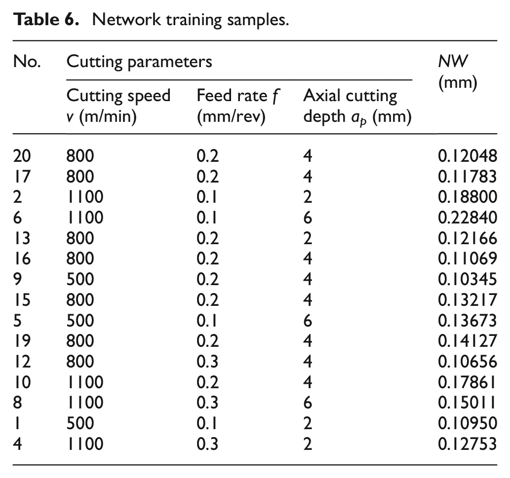
After the parameters of the GA-BP model were determined, 20 sets of test data obtained by the tool wear test were used as the network training and verification samples. In MATLAB software (version 2014 b), the rand function was used to randomly select 15 sets of data in Table 2 as the network training samples, as shown in Table 6. Before network training, the mapminmax function in MATLAB toolbox was used to normalise the test data and map the test data to the interval of [0, 1]. This process can reduce the errors caused by different orders of magnitude and dimensions, thereby avoiding neuron saturation and improving the convergence rate of neural network.

Table 6.

Network training samples.

No.	Cutting parameters			NW(mm)
No.	Cutting speed v (m/min)	Feed rate f(mm/rev)	Axial cuttingdepth a_p (mm)	NW(mm)
20	800	0.2	4	0.12048
17	800	0.2	4	0.11783
2	1100	0.1	2	0.18800
6	1100	0.1	6	0.22840
13	800	0.2	2	0.12166
16	800	0.2	4	0.11069
9	500	0.2	4	0.10345
15	800	0.2	4	0.13217
5	500	0.1	6	0.13673
19	800	0.2	4	0.14127
12	800	0.3	4	0.10656
10	1100	0.2	4	0.17861
8	1100	0.3	6	0.15011
1	500	0.1	2	0.10950
4	1100	0.3	2	0.12753

The network training parameters are set as follows: the maximum number of trainings is 200, the learning efficiency is 0.01, and the target mean square error (MSE) is 0.001. After a great deal of training, the unoptimised BPNN repeatedly falls into the local optimal solution and stops training when the number of training times and the target MSE are reached. The GA-BPNN can achieve the target MSE. The training results are stable.

Figure 12 shows the plots of training MSE of a random set of BPNN and GA-BPNN. As shown in Figure 12(a), BPNN stops training in the sixth epoch because it cannot jump out of the local optimal solution. The training MSE achieved is 0.22223, which is far from the target MSE. Figure 12(b) shows that after three iterations, the GA-BPNN reaches the training MSE of 0.017346, achieving the target MSE. These results indicate that the optimisation method using GA to find the optimal initial weight and threshold can improve the training speed and accuracy of BPNN, thereby confirming the feasibility of the model.

Figure 12.

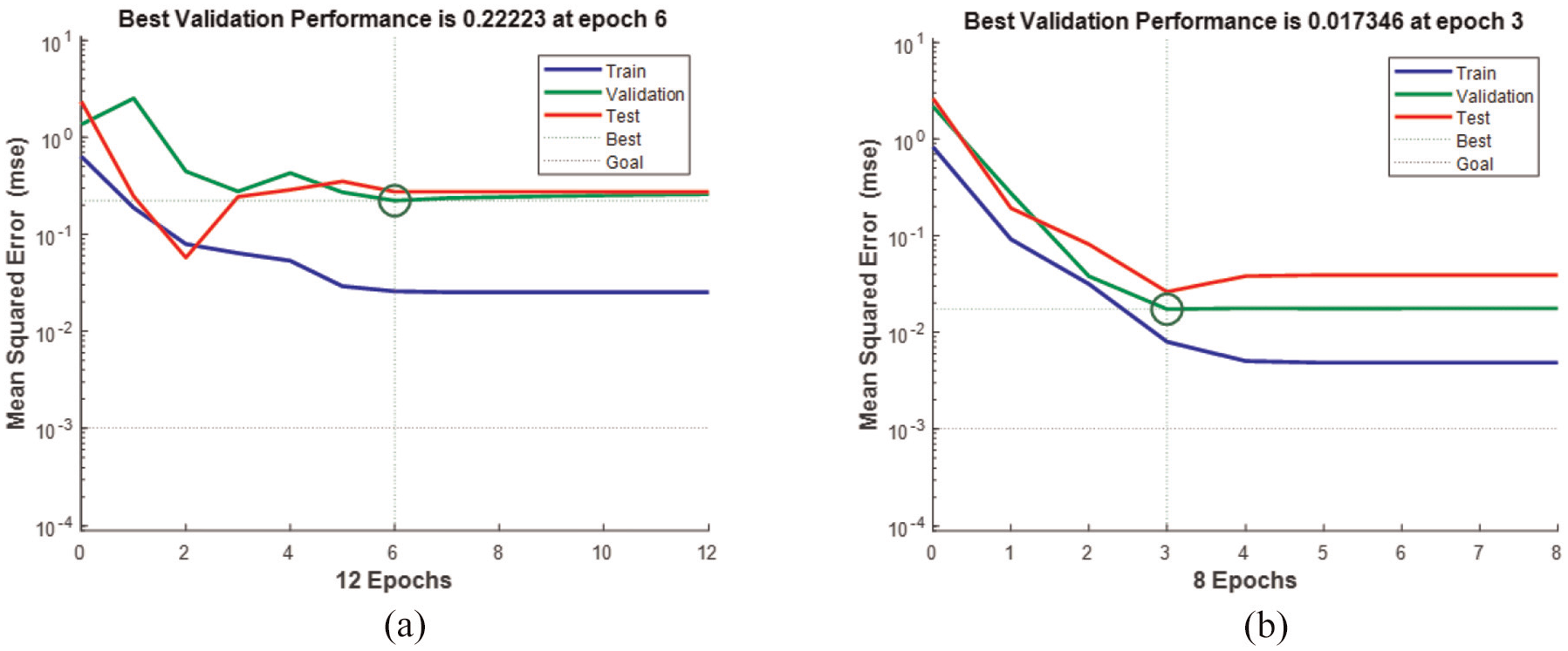
Comparison of MSE curves: (a) BPNN and (b) GA-BPNN.

Network generalisation verification

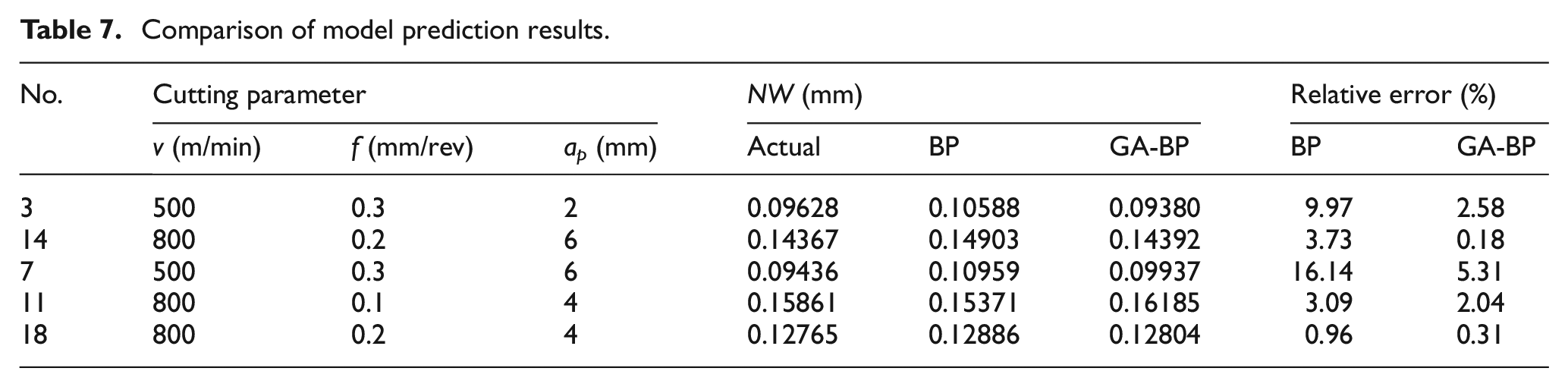
After the GA-BPNN prediction model was constructed through the network training process, the remaining five sets of experimental data in Table 1 were selected to conduct the generalisation verification of the established prediction model. As shown in Table 7, GA-BPNN has better prediction than the BPNN, and the relative error between the predicted value of GA-BP and the actual value is controlled within 5%.

Table 7.

Comparison of model prediction results.

No.	Cutting parameter			NW (mm)			Relative error (%)
No.	v (m/min)	f (mm/rev)	a_p (mm)	Actual	BP	GA-BP	BP	GA-BP
3	500	0.3	2	0.09628	0.10588	0.09380	9.97	2.58
14	800	0.2	6	0.14367	0.14903	0.14392	3.73	0.18
7	500	0.3	6	0.09436	0.10959	0.09937	16.14	5.31
11	800	0.1	4	0.15861	0.15371	0.16185	3.09	2.04
18	800	0.2	4	0.12765	0.12886	0.12804	0.96	0.31

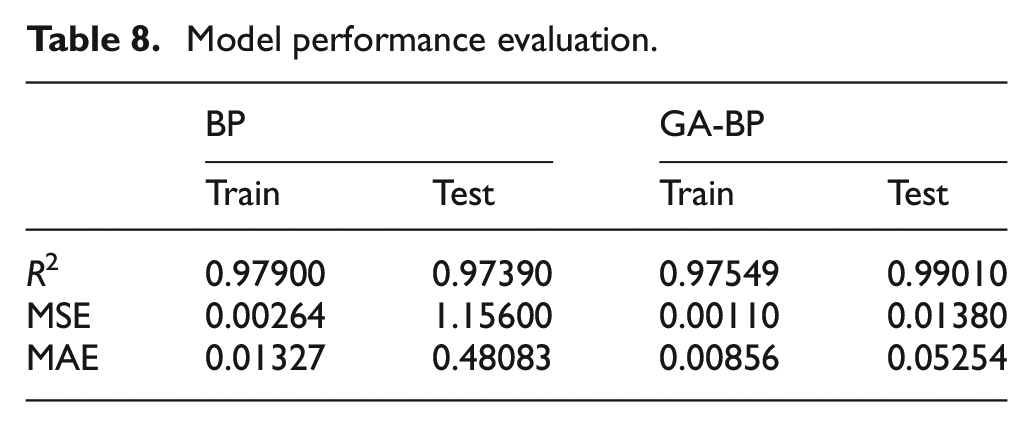
The model performance evaluation results are shown in Table 8. Figure 13 shows that GA-BPNN has a prediction determination coefficient of 99.01%, proving that the proposed GA-BP prediction model can predict effectively the tool wear during high-speed milling of WPCs.

Table 8.

Model performance evaluation.

	BP		GA-BP
	Train	Test	Train	Test
R ²	0.97900	0.97390	0.97549	0.99010
MSE	0.00264	1.15600	0.00110	0.01380
MAE	0.01327	0.48083	0.00856	0.05254

Figure 13.

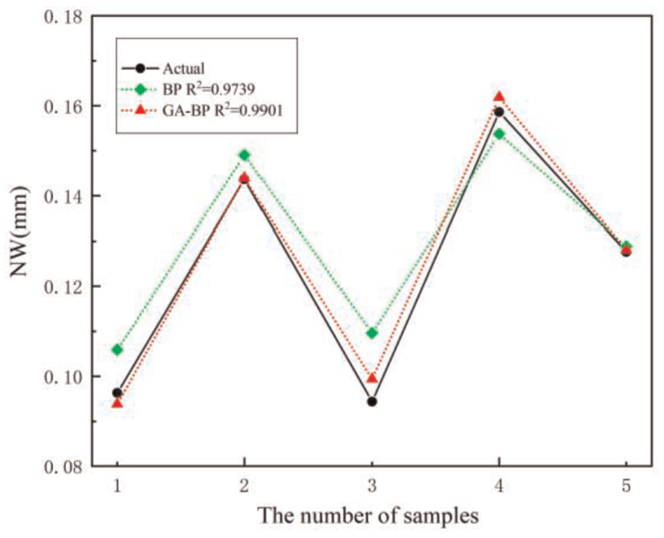
Generalisation verification of network.

Conclusions

After the initial weights and thresholds of the BPNN were optimised by using a GA, the inability of the traditional BPNN to jump out of the local minimum solution can be overcome effectively. The optimised BPNN has a faster convergence speed and better stability.

The model generalisation verification shows that the three-layer GA-BPNN prediction model established on MATLAB with cutting speed, feed rate and axial cutting depth as input variables and tool NW as output variable has good stability. It possesses few iterations and does not readily fall into the local optimal solution. The results show that the relative error between the predicted value and the actual value is controlled within 5%, and the coefficient of determination R² reaches 99.01%, which certainly has higher prediction accuracy than the traditional BPNN. Hence, the established GA-BPNN prediction model can well predict the tool wear during high-speed milling of WPCs, thereby providing guidance for tool wear prediction in the actual production process and significantly saves time and cost.

Footnotes

Declaration of conflicting interests

The author(s) declared no potential conflicts of interest with respect to the research, authorship, and/or publication of this article.

Funding

The author(s) disclosed receipt of the following financial support for the research, authorship, and/or publication of this article: This research was financially supported by the Jiangsu Key Laboratory of Precision and Micro-Manufacturing Technology (2019), Jiangsu ‘Six Talent Peak’ Project (JXQC-022).

ORCID iD

Weihua Wei

References

Wei

Xue

, et al. The research progress of machining mechanisms in milling wood-based materials. BioResources 2017; 13(1): 2139–2149.

Wen

. Intelligent fault diagnosis technology. Beijing: Beihang University Press, 2015. (in Chinese)

Moore

Stammers

Dominguez-Caballero

. The application of machine learning to sensor signals for machine tool and process health assessment. Proc IMechE, Part B: J Engineering Manufacture 2021; 235(10): 1543–1557.

Singh

Panda

Chakraborty

, et al. Predicting drill wear using an artificial neural network. Int J Adv Manuf Technol 2006; 28(5–6): 456–462.

Fan

Zheng

Cheng

, et al. Tool wear prediction when machining Ti6Al4V using different tool materials. In: 4th international conference on high speed machining, Guangzhou, China, March 2011.

Gao

Shen

Huang

, et al. Research of tool wear in BTA based on neural network. Tool Engineering 2016; 50(11): 107–109.

Quiza

Figueira

Paulo Davim

. Comparing statistical models and artificial neural networks on predicting the tool wear in hard machining D2 AISI steel. Int J Adv Manuf Technol 2008; 37(7–8): 641–648.

Paul

Varadarajan

. A multi-sensor fusion model based on artificial neural network to predict tool wear during hard turning. Proc IMechE, Part B: J Engineering Manufacture 2012; 226(5): 853–860.

Özel

Karpat

. Predictive modeling of surface roughness and tool wear in hard turning using regression and neural networks. Int J Mach Tools Manuf 2005; 45(4–5): 467–479.

10.

Mukherjee

Ray

. A review of optimization techniques in metal cutting processes. Comput Ind Eng 2006; 50(1–2): 15–34.

11.

Khajavi

Nasernia

Rostaghi

. Milling tool wear diagnosis by feed motor current signal using an artificial neural network. J Mech Sci Technol 2016; 30(11): 4869–4875.

12.

Chen

Jin

Jiri

. Predicting tool wear with multi-sensor data using deep belief networks. Int J Adv Manuf Technol 2018; 99(5–8): 1917–1926.

13.

Tang

Wang

, et al. Research on tool wear prediction based on deep residual network. In: 2018 3rd international workshop on materials engineering and computer sciences (IWMECS), Jinan, China, January 2018, pp.314–318.

14.

Srikant

Krishna

Rao

. Online tool wear prediction in wet machining using modified back propagation neural network. Proc IMechE, Part B: J Engineering Manufacture 2011; 225(7): 1009–1018.

15.

Xue

Wang

, et al. Tool life prediction based on particle swarm optimization–back-propagation neural network. Proc IMechE, Part B: J Engineering Manufacture 2015; 229(10): 1742–1752.

16.

Scheffer

Engelbrecht

Heyns

. A comparative evaluation of neural networks and hidden Markov models for monitoring turning tool wear. Neural Comput Appl 2005; 14(4): 325–336.

17.

Ojha

Dixit

. An economic and reliable tool life estimation procedure for turning. Int J Adv Manuf Technol 2005; 26(7–8): 726–732.

18.

Behera

Ghadai

Kalita

, et al. Simultaneous prediction of delamination and surface roughness in drilling GFRP composite using ANN. Int J Plast Technol 2016; 20(2): 424–450.

19.

Balazinski

Czogala

Jemielniak

, et al. Tool condition monitoring using artificial intelligence methods. Eng Appl Artif Intell 2002; 15(1): 73–80.

20.

Leung

Lam

Ling

, et al. Tuning of the structure and parameters of a neural network using an improved genetic algorithm. IEEE Trans Neural Netw 2003; 14(1): 79–88.

21.

Chen

Qian

, et al. A study on thermal performance of revolving heat pipe grinding wheel. Appl Therm Eng 2021; 182: 116065.

22.

Kalita

Shivakoti

Ghadai

. Optimizing process parameters for laser beam micro-marking using genetic algorithm and particle swarm optimization. Mater Manuf Process 2017; 32(10): 1101–1108.

23.

Liang

Liu

Wen

, et al. Effectiveness prediction of abrasive jetting stream of accelerator tank using normalized sparse autoencoder-adaptive neural fuzzy inference system. Proc IMechE, Part B: J Engineering Manufacture 2020; 234(13): 1615–1639.

24.

. Selection of initial weights and thresholds based on the Genetic Algorithm with the optimized Back-Propagation neural network. In: 2015 12th international conference on fuzzy systems and knowledge discovery (FSKD), Zhangjiajie, China, 15–17 August 2015, pp.173–177. New York: IEEE.

25.

Pang

Kuang

. The influence of cutting parameters on micro-topography of frequency features extracted from the machined KH₂PO₄ surfaces. Proc IMechE, Part B: J Engineering Manufacture 2020; 234(14): 1762–1770.

26.

Wang

Zhou

, et al. The finite element analysis–based simulation and artificial neural network–based prediction for milling processes of aluminum alloy 7050. Proc IMechE, Part B: J Engineering Manufacture 2021; 235(1–2): 265–277.

27.

Wang

. Tool wear prediction model based on GA-BP algorithm. Modular Machine Tool & Automatic Manufacturing Technique 2018; 10: 145–150.

28.

Kaya

Oysu

Ertunc

, et al. A support vector machine-based online tool condition monitoring for milling using sensor fusion and a genetic algorithm. Proc IMechE, Part B: J Engineering Manufacture 2012; 226(11): 1808–1818.

29.

Ghadai

Kalita

Mondal

, et al. Genetically optimized diamond-like carbon thin film coatings. Mater Manuf Process 2019; 34(13): 1476–1487.

30.

Kalita

Dey

Haldar

. Robust genetically optimized skew laminates. Proc IMechE, Part C: J Mechanical Engineering Science 2019; 233(1): 146–159.

31.

Elbaz

Shen

Zhou

, et al. Prediction of disc cutter life during shield tunneling with AI via the incorporation of a genetic algorithm into a GMDH-Type neural network. Engineering 2021; 7(2): 238–251.

32.

Kalita

Dey

Haldar

. Search for accurate RSM metamodels for structural engineering. J Reinforced Plast Compos 2019; 38(21–22): 995–1013.

33.

Yang

. Practical tutorial on artificial neural networks. Hangzhou: Zhejiang University Press, 2001. (in Chinese)

34.

Twardowski

Wiciak-Pikuła

. Prediction of tool wear using artificial neural networks during turning of hardened steel. Materials 2019; 12(19): 3091.

Prediction of tool wear based on GA-BP neural network

Abstract

Keywords

Introduction

Mathematical model of BPNN and GA

Mathematical model of BPNN

Mathematical model of GA-BPNN

Experiment of tool wear

Experiment preparation

Experimental equipment

Experimental tool

Experimental results of tool wear

Tool wear prediction model basedon GA-BPNN

Parameter setting of BPNN

Network structure parameters

Network structure function

Parameter setting of GA

Results and discussion

Network training

Network generalisation verification

Conclusions

Footnotes

Declaration of conflicting interests

Funding

ORCID iD

References