Development of the innovative differential tool wear modeling for high-feed milling and its experimental verification

Abstract

During the high-feed milling process, the vibrations generated by interrupted cutting cause changes in the instantaneous tool posture, as well as in the working angle and the distribution of the thermal stress coupling fields of each tool blade. These changes result in significant differences in the wear distribution of each tool blade. In this research, well-designed experiments for the high-feed milling of titanium alloys were carried out to identify the key factors affecting the differential wear on the milling tool insert blades. A differential tool wear model for the tool blades was developed in order to comprehensively describe the effects of the location error of the blades, the vibrations in the tool posture, and the working angle of each tool blade. The wear status of the milling tool was simulated based on the dynamic tool trajectories and postures derived by the model, and the entire simulated wear distribution was investigated with an innovative wear boundary recognition method. The differential tool wear model was evaluated and validated by the milling experiments and further supported by simulations.

Introduction

High-speed milling has been applied increasingly widely because of its superior machining efficiency and performance.^1,2 High-feed milling is a typical high-speed milling process, but it imposes unique industrial challenges, particularly for milling tools in terms of tool wear and machining dynamics. In high-feed milling processes, the structural rigidity and geometrical characteristics of a workpiece are varied, which tends to cause the vibrations of a milling tool. ³ The instantaneous tool posture and the working angle of the tool insert blades are also varied,^4,5 and the distribution of the thermal coupling fields of each blade is hence inconsistent in the process,^6,7 which leads to significant differences in the blade wear boundary and degrees (Figure 1). Therefore, it is difficult to obtain the effective prediction and control of the blades and the milling tool. Furthermore, because the machining accuracy and surface topography of different machining areas are likely to be inconsistent, the stability and reliability of the milling process will be low and, in turn, affect the machining efficiency and performance.^8–10

Figure 1.

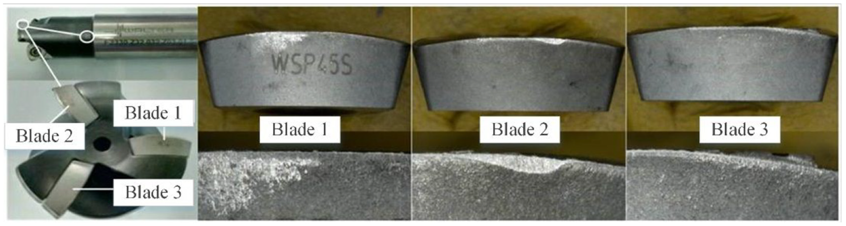
Flank wear on different tool insert blades for high-feed milling of titanium alloy.

Over the years, a number of researchers have carried out many meaningful studies on the differential wear of milling tools. For example, Girardin et al. ¹¹ detected the occurrence of tool wear by monitoring the variations of milling vibration signals. They presented the direct relationships among the tool wear, tool breakage, and milling vibrations. They also pointed out that the differences in the rotational frequency and the slow-down between teeth were a good indicator of the differential wear on the milling tool teeth. Zhao et al. ¹² researched the online grading evaluation of the tool wear degree and developed the non-linear mapping between the spindle motor current values and the tool wear under different cutting conditions. Xu et al. ¹³ comprehensively studied the flank wear distribution for tools turning large pitch threads. They also evaluated the difference in the left and right flank wear of a tool during different cutting conditions. Fang ¹⁴ presented the concept that in the layered mechanical milling process, a tool would produce uneven wear due to uneven cutting forces on the side of the tool. Hatt et al. ¹⁵ used a diffusion coupling model to study the effects of chemical factors on tool wear characteristics. It was revealed that in the processing of titanium alloys, the formation of TiC played a key role in reducing the differential tool wear. Wang ¹⁶ considered the critical temperature of a friction pair as the criterion for assessing the occurrence mechanisms of differential tool wear. Wang also developed a mathematical model of the milling tool wear. Zhang et al. ¹⁷ found that the wear increment of a tool was relatively stable at a high cutting speed, and the wear mechanism was mainly shock wear, while at a low cutting speed, the wear mechanism was mainly based on high-temperature adhesive wear. However, the above results related to the differential wear on tool cutting blades mainly rendered the experimental observations and the associated analysis. The key factors for the differential tool blade wear were not clearly identified. It is essential and much needed to have a scientific analysis for the differential tool wear in high-feed milling in order to establish a collective holistic understanding of the tool blade position errors, instantaneous cutting vibrations, distribution of the differential thermal stress coupling fields, and tool blade wear.

In this study, the high-feed milling experiments for titanium alloy are presented first. These experiments were carried out to identify the key factors that affected the differential wear for the high-feed milling tool blades. The effects of the tool posture, instantaneous working angle of each tool blade, and the consequent vibrations were clarified, and the changes in the distribution of the thermal stress fields were studied. The wear status of the milling tool was simulated based on the dynamic tool trajectories and postures that were derived with the modeling and analysis, and the complete simulated wear distributions were investigated with a comprehensive wear boundary recognition method. Finally, the differential tool wear model was validated and verified by well-designed high-feed milling experiments.

Factors affecting the differential wear on tool insert blades in high-feed milling

In order to identify the factors affecting the differential wear at the tool blades, 10 sets of high-feed milling experiments for a titanium alloy were carried out on a three-axis milling machining center (VDL-1000E). Additionally, in order to clearly observe the wear differences of the blades, a proper milling distance had to be selected. Kuppuswamy et al.^18,19 reported that the growth of the flank wear was erratic and rapid at the first 10−25 m of cutting distance. The cutting tool used in this work was a high-feed milling cutter, the diameter of which was 32 mm. Due to the high machining efficiency, it was believed that the wear differences of the blades were much easier to observe. The cutting distances (L) were chosen as 0.5 m, 1 m, …, 5 m. The spindle rotation speed (n) used in the experiment was 1143 r/min, the feed speed (v_f) was 500 mm/min, the milling depth (a_p) was 0.5 mm, and the milling width (a_e) was 16 mm. The milling tool structure and the configuration are shown in Figure 2.

Figure 2.

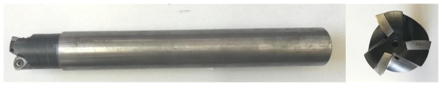
Illustration of the high-feed milling cutter.

Before the start of each set of experiments, three blades were numbered separately for further research on the wear difference, and the tool was measured to determine the axial position error $(\mathrm{\Delta }{c}_{\min }^j)$ and the radial position error $(\mathrm{\Delta }{r}_0^j)$ of the milling tool blade. The measurement method for the blade errors is shown in Figure 3. The blade error measurement results are listed in Table 1.

Figure 3.

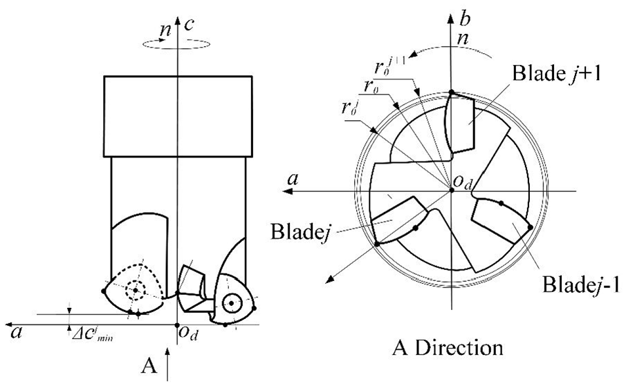
Schematic view of the measurement of blade errors.

Table 1.

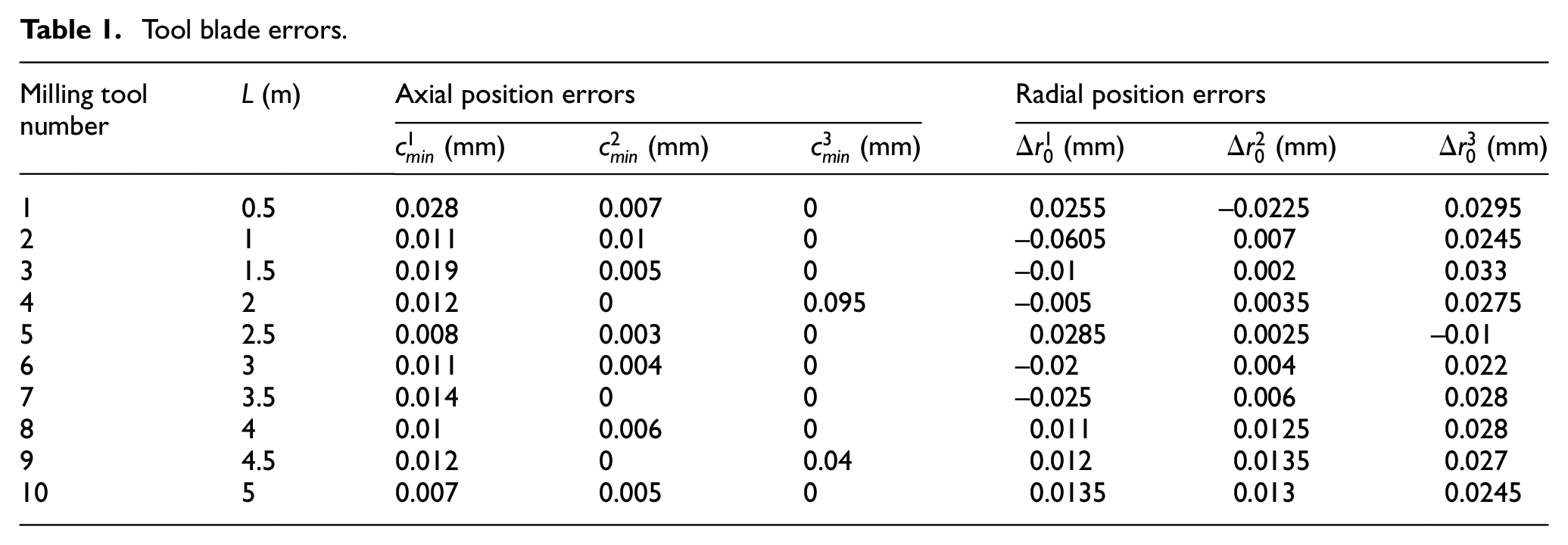
Tool blade errors.

Milling tool number	L (m)	Axial position errors			Radial position errors
		$c_{\min }^1(\mathrm{mm})$	$c_{\min }^2(\mathrm{mm})$	$c_{\min }^3(\mathrm{mm})$	$\mathrm{\Delta }{r}_0^1(\mathrm{mm})$	$\mathrm{\Delta }{r}_0^2(\mathrm{mm})$	$\mathrm{\Delta }{r}_0^3(\mathrm{mm})$
1	0.5	0.028	0.007	0	0.0255	−0.0225	0.0295
2	1	0.011	0.01	0	−0.0605	0.007	0.0245
3	1.5	0.019	0.005	0	−0.01	0.002	0.033
4	2	0.012	0	0.095	−0.005	0.0035	0.0275
5	2.5	0.008	0.003	0	0.0285	0.0025	−0.01
6	3	0.011	0.004	0	−0.02	0.004	0.022
7	3.5	0.014	0	0	−0.025	0.006	0.028
8	4	0.01	0.006	0	0.011	0.0125	0.028
9	4.5	0.012	0	0.04	0.012	0.0135	0.027
10	5	0.007	0.005	0	0.0135	0.013	0.0245

During the experiments with milling titanium alloy, the vibration signals that were generated by the cutting force were detected. Other research studies have indicated that compared with flank wear, rear wear has a dominant effect on the machined surface qualities and cutting force, ²⁰ and the flank wear differences were not taken into consideration in this work.

In order to accurately describe the difference in the wear distributions of different tool blades, after the experiments, an ultra-depth microscope was used to detect the upper and lower boundaries of the wear area of each high-feed milling tool blade. The wear area images of the flank face of the blade bottom were obtained with different cutting distances.

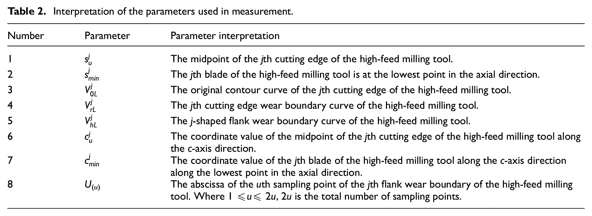
After obtaining the wear area images, the data points that were used for further fitting of the wear boundary curves could be derived. The projection of the unworn tip on the mounting surface of the blade was taken as the coordinate origin, and the measurement coordinate was thus established. The number and the measurement coordinates of milling tool blades are shown in Figure 4, and the method for determining the upper and lower boundaries of the tool blade wear area is shown in Figure 5. The horizontal distance between the point $s_{\min }^j$ and the point $s_u^j$ was taken as the sampling point interval, and using this interval, the projection of the cutting edge on the U axis was equally spaced. The data points for fitting the wear boundary curves could thus be treated as the intersection points between the vertical lines through U₍₁₎, U₍₂₎, …, U_(2U) and the original cutting edge curve, the upper wear boundary curve, and the lower wear boundary curve. The parameter interpretation used in Figure 5 is shown in Table 2.

Figure 4.

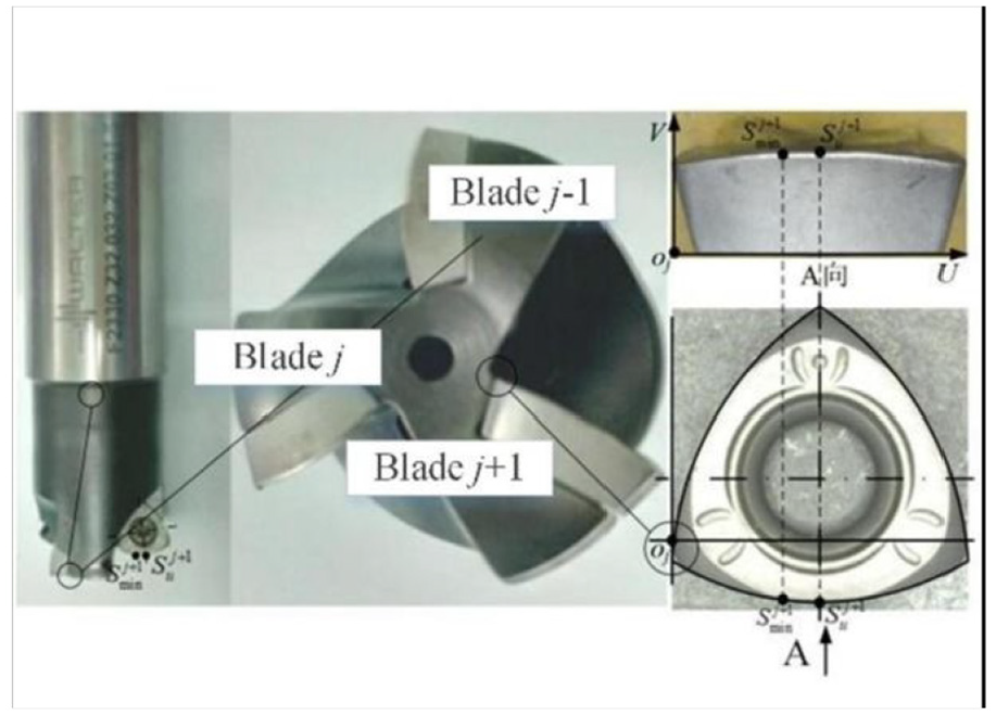
Measurement coordinates for the milling tool blades.

Figure 5.

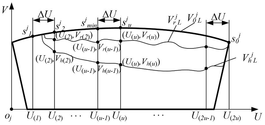
Measurement method for the data points fitting wear boundaries of the tool blade.

Table 2.

Interpretation of the parameters used in measurement.

Number	Parameter	Parameter interpretation
1	$s_u^j$	The midpoint of the jth cutting edge of the high-feed milling tool.
2	$s_{\min }^j$	The jth blade of the high-feed milling tool is at the lowest point in the axial direction.
3	$V_{0L}^j$	The original contour curve of the jth cutting edge of the high-feed milling tool.
4	$V_{\mathrm{rL}}^j$	The jth cutting edge wear boundary curve of the high-feed milling tool.
5	$V_{\mathrm{hL}}^j$	The j-shaped flank wear boundary curve of the high-feed milling tool.
6	$c_u^j$	The coordinate value of the midpoint of the jth cutting edge of the high-feed milling tool along the c-axis direction.
7	$c_{\min }^j$	The coordinate value of the jth blade of the high-feed milling tool along the c-axis direction along the lowest point in the axial direction.
8	U (u)	The abscissa of the uth sampling point of the jth flank wear boundary of the high-feed milling tool. Where 1 ≤u≤ 2u, 2u is the total number of sampling points.

After acquiring the data points and their coordinates, MATLAB programming was used to perform the binary high-order polynomial fitting. Therefore, the original cutting edge boundary equation of the cutting edge of the high-feed milling tool, the upper wear boundary equation of the tool cutting edge, and the lower wear boundary equation were obtained, as shown in equations (1)–(3)

$$V_{0L}=\sum _{i=0}^M{P}_i{U}^i$$

(1)

$$V_{\mathrm{rL}}^j=\sum _{i=0}^M\sum _{k=0}^N{P}_{\mathrm{ik}}^{\mathrm{rj}}{U}^i{L}^k$$

(2)

$$V_{\mathrm{hL}}^j=\sum _{i=0}^M\sum _{k=0}^N{P}_{\mathrm{ik}}^{\mathrm{rj}}{U}^i{L}^k$$

(3)

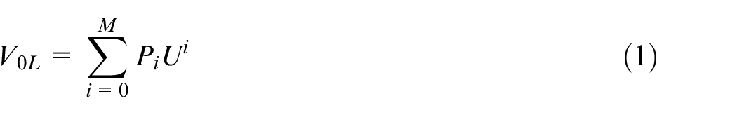
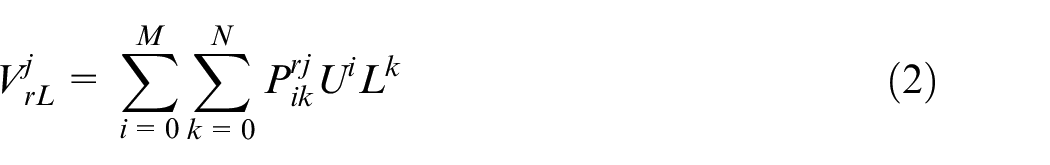
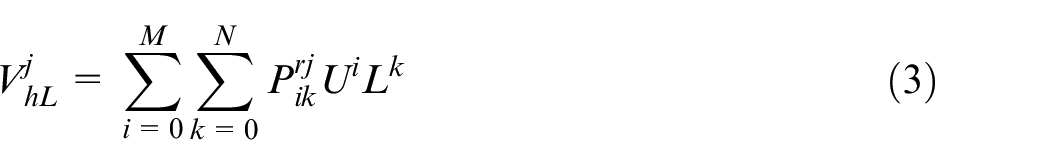
where M is the highest power of U in the wear boundary equation, N is the highest power of V in the wear boundary equation, $P_{\mathrm{ik}}^{\mathrm{rj}}$ is the coefficient in the wear boundary equation of the cutting edge, and $P_{\mathrm{ik}}^{\mathrm{hj}}$ is the flank wear boundary equation coefficient.

Using the above method, the wear distributions of all of the milling tool blades at any milling distances could be obtained. The wear images at a milling distance of 2.5 m are shown in Figure 6.

Figure 6.

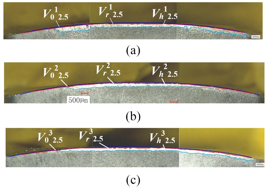
Wear distribution on three tool blades with the milling distance of 2.5 m: (a) blade 1, (b) blade 2, and (c) blade 3.

It can be observed from Figure 6 that there were obvious differences for the wear width of the three blades. Among the three blades, the maximum wear width of blade 1 was the largest, while that of blade 3 is the smallest. Additionally, the position of the maximum wear width for blades 1 and 2 was near to the milling tool tip, while the position for blade 3 was far away from that. The blade with the maximum radial error (blade 1, 0.0285 mm) had the maximum wear width, and the position of the maximum wear width of the blade with the maximum axial error (blade 1, 0.008 mm) was nearest to the blade tip. Thus, the differences in the wear width were caused by blade errors, and once the initial blade position deviated from its designed position, the contact area, cutting force, and corresponding milling vibration consequently became large. The stress and the temperature also become larger than those of the other blades. Finally, the wear was more severe than that of the other blades.

In order to comprehensively describe the evolution of the difference in the wear distribution of the milling tool with the increase in the milling distance, the changes of the wear distribution on the flank face of the single-tool blade with the cutting distance, the error distribution of the tool blades, and the milling vibration had to be investigated. ²¹ In order to describe these changes, two kinds of specific parameters were defined.

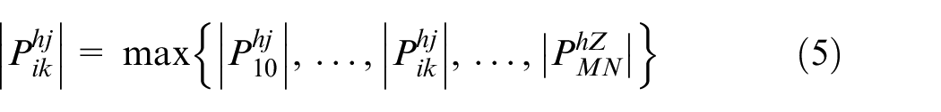
The two coefficients with the largest absolute values of the blade cutting edge upper and lower boundary equations were taken as the two specific parameters of the wear boundary curves of the cutting edge upper boundary and the lower boundary of each blade, as shown in equations (4) and (5)

$$\left|P_{\mathrm{ik}}^{\mathrm{rj}}\right|=\max \{\left|P_{10}^{\mathrm{rj}}\right|,\dots ,\left|P_{\mathrm{ik}}^{\mathrm{rj}}\right|,\dots ,\left|P_{\mathrm{MN}}^{\mathrm{rj}}\right|\}$$

(4)

$$\left|P_{\mathrm{ik}}^{\mathrm{hj}}\right|=\max \{\left|P_{10}^{\mathrm{hj}}\right|,\dots ,\left|P_{\mathrm{ik}}^{\mathrm{hj}}\right|,\dots ,\left|P_{\mathrm{MN}}^{\mathrm{hZ}}\right|\}$$

(5)

Using the above method, the parameters $P_{11}^{\mathrm{rj}}$ , $P_{12}^{\mathrm{rj}}$ , $P_{10}^{\mathrm{rj}}$ (j = 1, 2, 3) and $P_{11}^{\mathrm{hj}}$ , $P_{10}^{\mathrm{hj}}$ , $P_{12}^{\mathrm{hj}}$ (j = 1, 2, 3) were taken as examples to obtain the wear boundary curves of the tool cutting edge in different milling distances. The changing law of the upper and lower wear boundary curves of the different tool blades could thus be shown as seen in Figures 7 and 8.

Figure 7.

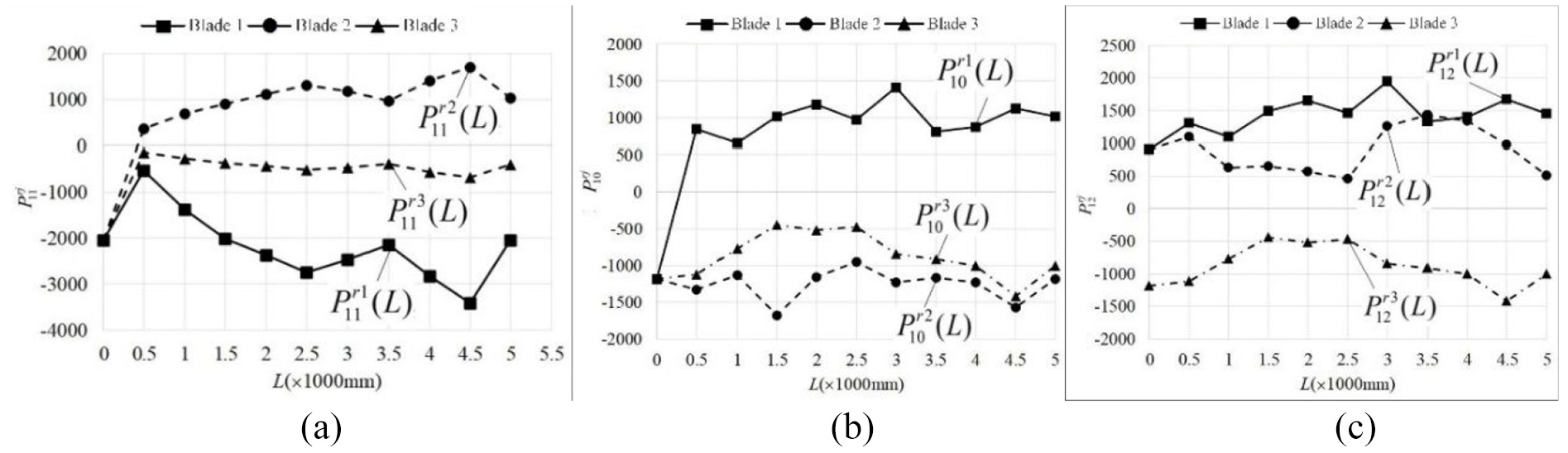
The changing law of the upper wear boundaries curves of the different tool blades: (a) $P_{11}^{\mathrm{rj}}$ , (b) $P_{12}^{\mathrm{rj}}$ , and (c) $P_{10}^{\mathrm{rj}}$ .

Figure 8.

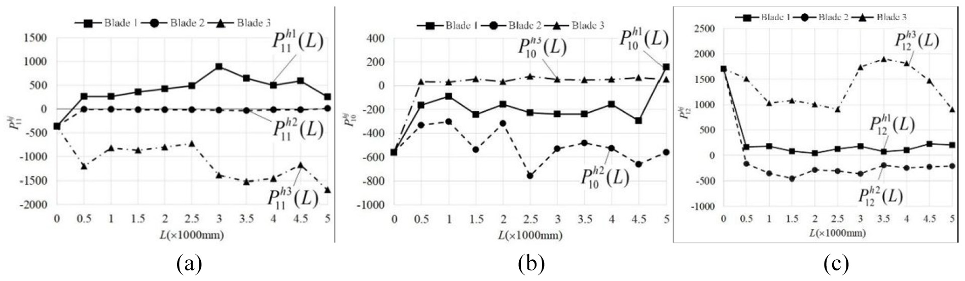
The changing law of the lower wear boundaries curves of the different tool blades: (a) $P_{11}^{\mathrm{hj}}$ , (b) $P_{10}^{\mathrm{hj}}$ , and (c) $P_{12}^{\mathrm{hj}}$ .

It can be seen from Figure 7 that the parameters $P_{11}^{\mathrm{rj}}$ , $P_{12}^{\mathrm{rj}}$ , and $P_{10}^{\mathrm{rj}}$ exhibited different variations with the cutting distance. Furthermore, the values of $P_{11}^{r1}$ , $P_{11}^{r2}$ , and $P_{11}^{r3}$ were at different levels. The variations of $P_{10}^{r2}$ and $P_{10}^{r3}$ were similar and different from that of $P_{10}^{r1}$ . The variations of $P_{12}^{r1}$ and $P_{12}^{r2}$ were similar and different from that of $P_{12}^{r3}$ .

It can be seen from Figure 8 that the parameters $P_{11}^{\mathrm{hj}}$ , $P_{10}^{\mathrm{hj}}$ , and $P_{12}^{\mathrm{hj}}$ exhibited different variations with the cutting distance, and the values of $P_{11}^{h1}$ , $P_{11}^{h2}$ , and $P_{11}^{h3}$ were at different levels. The changes of $P_{10}^{h1}$ and $P_{10}^{h2}$ were very similar, while $P_{10}^{h3}$ stayed around a constant value of zero. The variation of $P_{12}^{h1}$ was close to that of $P_{12}^{h2}$ , while $P_{12}^{h3}$ had a big fluctuation.

Based on the above analysis, it was believed that not only the maximum wear width and its position but also the whole distribution of the three blades were different. Since the milling parameters were constant in the experiments, the reasons for the differential wear distribution were the initial blade errors and the dynamic milling vibration.

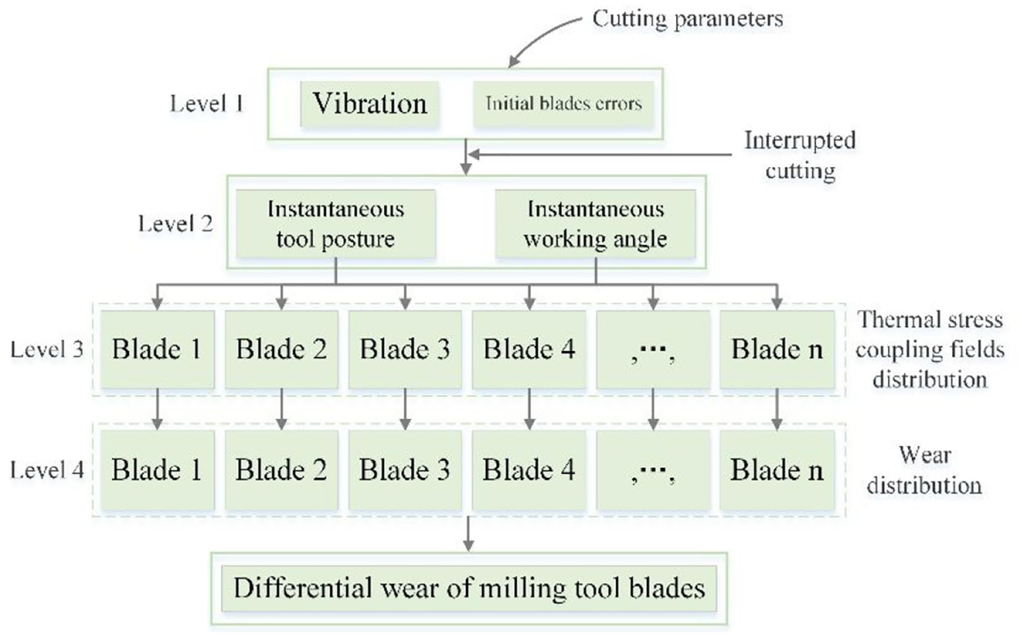
The above results showed that the method for identifying the key influencing factors on the tool blade wear in high-feed milling could accurately and comprehensively identify the factors affecting the wear distribution of the tool blades in the milling process. A brief summary of the relationship between these factors and the wear distribution is shown in Figure 9.

Figure 9.

Relationship between the influence factors and wear distribution.

In Figure 9, the cutting parameters are those that could be controlled, but could not directly affect wear distribution of tool blades (Level 4). These cutting parameters could only directly control the vibration (Level 1). Additionally, the changes in the wear distribution were due to the distribution of the thermal stress coupling fields (Level 3) which was caused by the instantaneous tool posture and the working angle (Level 2). Thus, in order to further clarify how these factors affected the wear distribution of the tool blades, the analytical differential wear analysis models had to be developed first in order to clarify the relationship between the vibration (Level 1) and the instantaneous tool posture and working angle (Level 2). Then, the relationship between Levels 2 and 3 could be investigated by simulation analysis.

Modeling and analysis of differential tool wear in high-feed milling

Effect of vibration on the instantaneous tool posture and working angle (Level 1–Level 2)

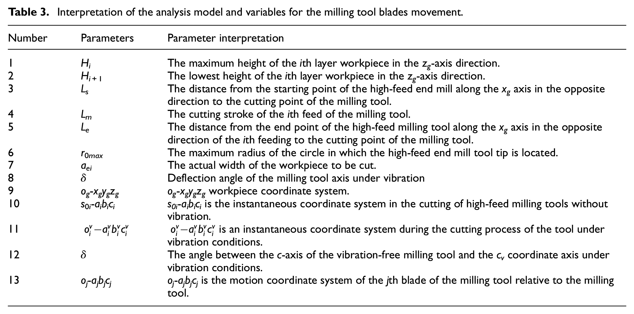
In order to clarify the effect of the milling vibration (Level 1 in Figure 9) on the instantaneous tool postures and the working angles (Level 2 in Figure 9) of the different blades, a cutting model was developed, as shown in Figure 10. The interpretation of the parameters in Figure 10 is further highlighted in Table 3.

Figure 10.

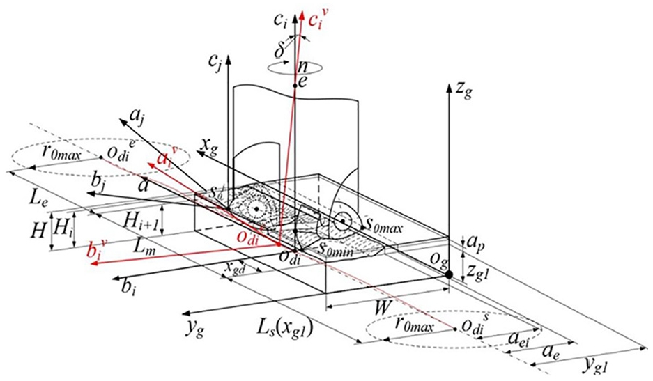
Cutting model of the high-feed milling tool.

Table 3.

Interpretation of the analysis model and variables for the milling tool blades movement.

Number	Parameters	Parameter interpretation
1	Hi	The maximum height of the ith layer workpiece in the zg-axis direction.
2	Hi+ 1	The lowest height of the ith layer workpiece in the zg-axis direction.
3	Ls	The distance from the starting point of the high-feed end mill along the xg axis in the opposite direction to the cutting point of the milling tool.
4	Lm	The cutting stroke of the ith feed of the milling tool.
5	Le	The distance from the end point of the high-feed milling tool along the xg axis in the opposite direction of the ith feeding to the cutting point of the milling tool.
6	r 0max	The maximum radius of the circle in which the high-feed end mill tool tip is located.
7	aei	The actual width of the workpiece to be cut.
8	δ	Deflection angle of the milling tool axis under vibration
9	og-xgygzg	og-xgygzg workpiece coordinate system.
10	s 0i-aibici	s0i-aibici is the instantaneous coordinate system in the cutting of high-feed milling tools without vibration.
11	$o_i^v-a_i^v{b}_i^v{c}_i^v$	$o_i^v-a_i^v{b}_i^v{c}_i^v$ is an instantaneous coordinate system during the cutting process of the tool under vibration conditions.
12	δ	The angle between the c-axis of the vibration-free milling tool and the cv coordinate axis under vibration conditions.
13	oj-ajbjcj	oj-ajbjcj is the motion coordinate system of the jth blade of the milling tool relative to the milling tool.

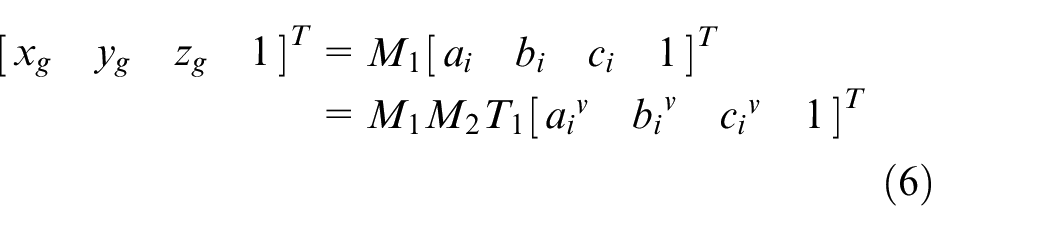
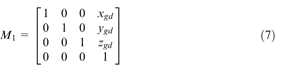
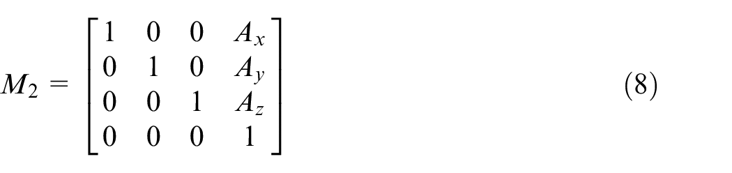
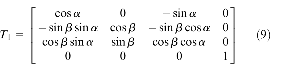
The coordinate transformation between the coordinate systems $o_d^v-a_i^v{b}_i^v{c}_i^v$ , o_d-a_ib_ic_i, o_g-x_gy_gz_g was as shown in equation (6). Furthermore, the transformation matrixes M₁ and M₂ could be written as equation (7) and (8), respectively. The transformation matrix T₁ is shown in equation (9)

$$\begin{array}{c}\multicolumn{1}{c}{{\left[\begin{array}{cccc}{x}_g\hfill & y_g\hfill & z_g\hfill & 1\hfill \end{array}\right]}^T=M_1{\left[\begin{array}{cccc}{a}_i\hfill & b_i\hfill & c_i\hfill & 1\hfill \end{array}\right]}^T}\\ =M_1{M}_2{T}_1{\left[\begin{array}{cccc}{a_i}^v\hfill & {b_i}^v\hfill & {c_i}^v\hfill & 1\hfill \end{array}\right]}^T\hfill \end{array}$$

(6)

$$M_1=\left[\begin{array}{cccc}1\hfill & 0\hfill & 0\hfill & x_{\mathrm{gd}}\hfill \\ \multicolumn{1}{c}{0}& 1\hfill & 0\hfill & y_{\mathrm{gd}}\hfill \\ \multicolumn{1}{c}{0}& 0\hfill & 1\hfill & z_{\mathrm{gd}}\hfill \\ \multicolumn{1}{c}{0}& 0\hfill & 0\hfill & 1\hfill \end{array}\right]$$

(7)

$$M_2=\left[\begin{array}{cccc}1\hfill & 0\hfill & 0\hfill & A_x\hfill \\ \multicolumn{1}{c}{0}& 1\hfill & 0\hfill & A_y\hfill \\ \multicolumn{1}{c}{0}& 0\hfill & 1\hfill & A_z\hfill \\ \multicolumn{1}{c}{0}& 0\hfill & 0\hfill & 1\hfill \end{array}\right]$$

(8)

$$T_1=\left[\begin{array}{cccc}\cos \alpha \hfill & 0\hfill & -\sin \alpha \hfill & 0\hfill \\ \multicolumn{1}{c}{-\sin \beta \sin \alpha }& \cos \beta \hfill & -\sin \beta \cos \alpha \hfill & 0\hfill \\ \multicolumn{1}{c}{\cos \beta \sin \alpha }& \sin \beta \hfill & \cos \beta \cos \alpha \hfill & 0\hfill \\ \multicolumn{1}{c}{0}& 0\hfill & 0\hfill & 1\hfill \end{array}\right]$$

(9)

The milling tool movement trajectories in three directions with vibration are shown in equation (10)

$$\{\begin{array}{c}{x}_{\mathrm{gd}}^v=v_f(t-(i-1)t_e)-x_{g1}-(i-1)(L_m+l_e)+A_x,t\in T_i\hfill \\ \multicolumn{1}{c}{y_{\mathrm{gd}}^v=W+r_{0\max }-a_{\mathrm{ei}}+A_y}\\ \multicolumn{1}{c}{z_{\mathrm{gd}}^v=H_0-i·a_p+A_z}\end{array}$$

(10)

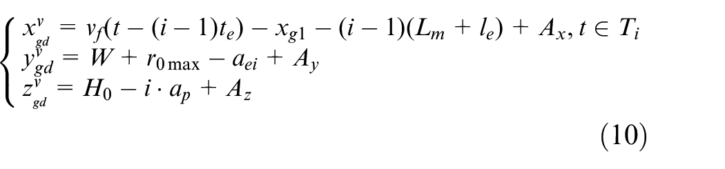
where t_e is the time for changing cutting path, that is, the time taken for the milling tool to move from o_dm-1 ^e to $o_{\mathrm{dm}}^s$ , and T_i is the cutting time of the ith feeding of the milling tool along the x_g axis. T_i could be expressed by equation (11)

$$T_i=[T_{\mathrm{is}},T_{\mathrm{ie}}]=[(i-1)(T_c+t_e),i{T}_c+(i-1)t_e]$$

(11)

$$T_c=\frac{x_{g1}+L_m+L_e}{v_f}$$

(12)

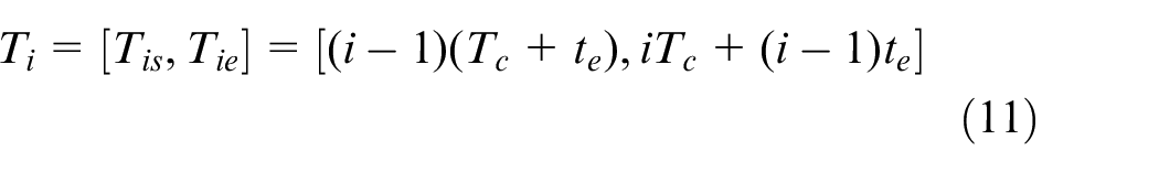
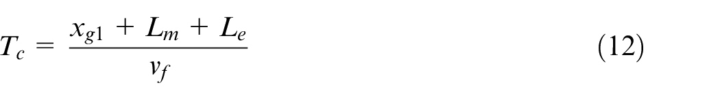
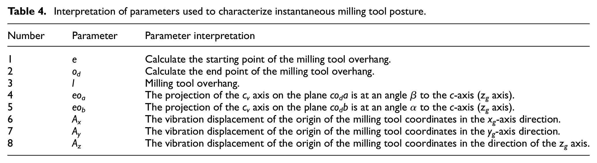
In order to characterize the instantaneous milling tool posture, the variables of the milling tool vibration in the time domain were introduced. Thus, the influence of the milling vibration on the instantaneous milling tool posture could be as shown in Figure 11. The corresponding interpretation of the parameters is listed in Table 4.

Figure 11.

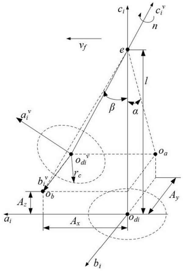
The instantaneous milling tool posture with vibrations.

Table 4.

Interpretation of parameters used to characterize instantaneous milling tool posture.

Number	Parameter	Parameter interpretation
1	e	Calculate the starting point of the milling tool overhang.
2	od	Calculate the end point of the milling tool overhang.
3	l	Milling tool overhang.
4	eoa	The projection of the cv axis on the plane coda is at an angle β to the c-axis (zg axis).
5	eob	The projection of the cv axis on the plane codb is at an angle α to the c-axis (zg axis).
6	Ax	The vibration displacement of the origin of the milling tool coordinates in the xg-axis direction.
7	Ay	The vibration displacement of the origin of the milling tool coordinates in the yg-axis direction.
8	Az	The vibration displacement of the origin of the milling tool coordinates in the direction of the zg axis.

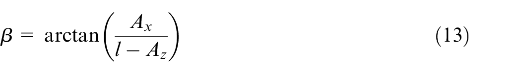
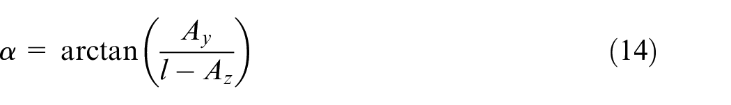
The parameters β (inclination angle of milling tool along feed direction) and α (inclination angle of the milling tool along the radial direction) that could characterize the instantaneous milling tool posture with vibration could be written as equations (13) and (14)

$$\beta =\arctan \left(\frac{A_x}{l-A_z}\right)$$

(13)

$$\alpha =\arctan \left(\frac{A_y}{l-A_z}\right)$$

(14)

Effect of the instantaneous tool posture and the working angle on the distribution of the thermal stress coupling fields (Levels 2–3)

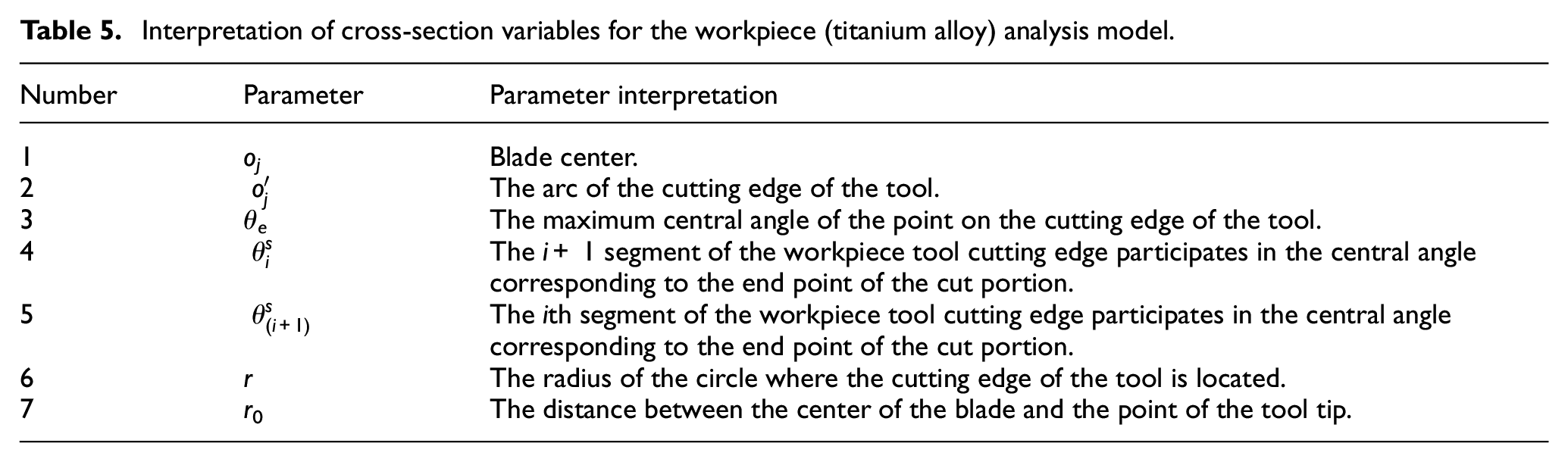
In the actual high-feed milling process, the contact depth between the tool blades and the workpiece always increased non-linearly. This was because the milling depth was usually small, while the feed rate was large, and the blade could not entirely be in contact with the workpiece for the first movement. In addition, the effective milling time was reduced due to the tool movement from the end of first feed to the start of the second feed, and the heat dissipation thus increased. These factors also had a significant effect on the distribution of the thermal stress coupling fields of the tool blades. Therefore, after describing the dynamic cutting behavior of the milling tool blades, according to the milling tool feed movement and the changes in the effective cutting time, the workpiece model was reconstructed in order to adapt to the variation of the distribution of the thermal stress coupling fields of each blade. The reconstructed model with consideration of the non-linear changes of the contact depth is shown in Figure 12, and its cross-sectional view is shown in Figure 13. The interpretation of the parameters used for characterization is listed in Table 5.

Figure 12.

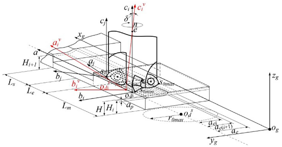
Reconstructed workpiece model for the first time.

Figure 13.

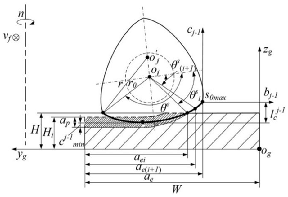
Cross-sectional view of the workpiece model for the first time.

Table 5.

Interpretation of cross-section variables for the workpiece (titanium alloy) analysis model.

Number	Parameter	Parameter interpretation
1	oj	Blade center.
2	$o{\prime }_j$	The arc of the cutting edge of the tool.
3	θe	The maximum central angle of the point on the cutting edge of the tool.
4	${\theta }_i^s$	The i+ 1 segment of the workpiece tool cutting edge participates in the central angle corresponding to the end point of the cut portion.
5	${\theta }_{(i+1)}^s$	The ith segment of the workpiece tool cutting edge participates in the central angle corresponding to the end point of the cut portion.
6	r	The radius of the circle where the cutting edge of the tool is located.
7	r 0	The distance between the center of the blade and the point of the tool tip.

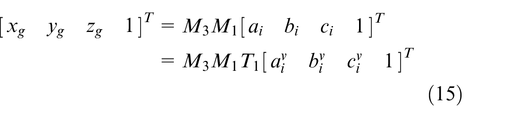
The transformation between the coordinate system of the milling tool and the workpiece coordinate system with vibration is shown in equation (15). The transformation matrixes M₃ and M₁ could be written as equations (16) and (17), respectively

$$\begin{array}{c}\multicolumn{1}{c}{{\left[\begin{array}{cccc}{x}_g\hfill & y_g\hfill & z_g\hfill & 1\hfill \end{array}\right]}^T=M_3{M}_1{\left[\begin{array}{cccc}{a}_i\hfill & b_i\hfill & c_i\hfill & 1\hfill \end{array}\right]}^T}\\ =M_3{M}_1{T}_1{\left[\begin{array}{cccc}{a}_i^v\hfill & b_i^v\hfill & c_i^v\hfill & 1\hfill \end{array}\right]}^T\hfill \end{array}$$

(15)

$$M_3=\left[\begin{array}{cccc}1\hfill & 0\hfill & 0\hfill & v_f·T_i\hfill \\ \multicolumn{1}{c}{0}& 1\hfill & 0\hfill & 0\hfill \\ \multicolumn{1}{c}{0}& 0\hfill & 1\hfill & -i·a_p\hfill \\ \multicolumn{1}{c}{0}& 0\hfill & 0\hfill & 1\hfill \end{array}\right]$$

(16)

$$M_1=\left[\begin{array}{cccc}1\hfill & 0\hfill & 0\hfill & x_d\hfill \\ \multicolumn{1}{c}{0}& 1\hfill & 0\hfill & y_d\hfill \\ \multicolumn{1}{c}{0}& 0\hfill & 1\hfill & z_d\hfill \\ \multicolumn{1}{c}{0}& 0\hfill & 0\hfill & 1\hfill \end{array}\right]$$

(17)

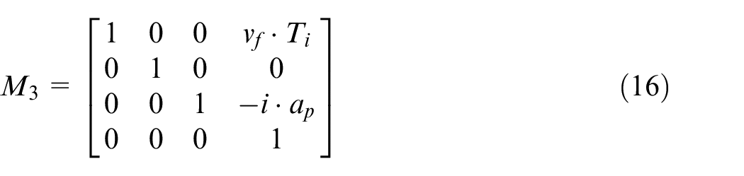
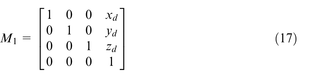
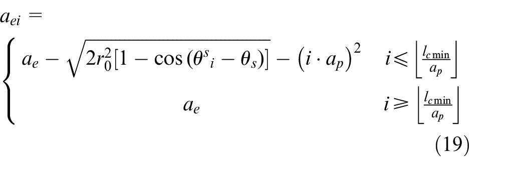
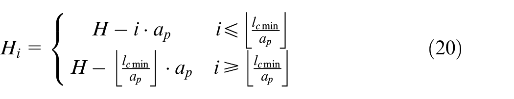
The parameters for characterizing the workpiece structure could be derived as equations (18)–(20)

$$L_m+L_s+L_e=v_f·T_c$$

(18)

$$\begin{array}{c}{a}_{\mathrm{ei}}=\hfill \\ \{\begin{array}{cc}{a}_e-\sqrt{2r_0^2[1-\cos ({{\theta }^s}_i-{\theta }_s)]}-{(i·a_p)}^2\hfill & i\le \lfloor \frac{l_{c\min }}{a_p}\rfloor \hfill \\ \multicolumn{1}{c}{a_e}& i⩾\lfloor \frac{l_{c\min }}{a_p}\rfloor \hfill \end{array}\hfill \end{array}$$

(19)

$$H_i=\{\begin{array}{cc}H-i·a_p\hfill & i\le \lfloor \frac{l_{c\min }}{a_p}\rfloor \hfill \\ \multicolumn{1}{c}{H-\lfloor \frac{l_{c\min }}{a_p}\rfloor ·a_p}& i⩾\lfloor \frac{l_{c\min }}{a_p}\rfloor \hfill \end{array}$$

(20)

$$l_{c\min }=l_c^j+{c^j}_{\min }$$

(21)

Furthermore, by taking the non-effective cutting time of the milling tool into consideration, the workpiece model was reconstructed for the second time, as shown in Figure 14.

Figure 14.

Reconstructed method of the workpiece for second time.

In Figure 14, q is a random selected point on the outer boundary of the workpiece, e(t₁) is the intersection of the $c_i^v$ axis and the c_i axis corresponding to point q, $f(x_{\mathrm{gd}}^v,y_{\mathrm{gd}}^v,z_{\mathrm{gd}}^v)=0$ represents the milling tool trajectories, $f(x_{\mathrm{gd}}^v,y_{\mathrm{gd}}^v,z_{\mathrm{gd}}^v+l)=0$ is the trajectory of the point e, α′(t₁) is the inclination angle of the milling tool along the feed direction, and β′(t₁) is the inclination angle of the milling tool along the radial direction.

According to the above reconstructing method, titanium alloy was chosen as the workpiece material, and UG modeling software was used to perform the finite element modeling, as shown in Figure 15.

Figure 15.

Reconstructed workpiece modeled by the UG tool.

It can be seen from the above results that the reconstructed workpiece model had specific geometrical features that exhibited many differences from a simple block. It was believed that the proposed analytical models could reflect the effect of the vibration (Level 1 in Figure 9) on the distribution of the thermal stress coupling fields (Level 3 in Figure 9). In order to validate the models proposed above, some simulation analyses of the distribution of the thermal stress coupling fields needed to be performed using the reconstructed workpiece model.

Verification of the differential tool wear models

Simulation of the wear distribution for the milling tool blades (Level 3–Level 4)

In order to obtain the distributions of the thermal stress coupling fields and the wear of the milling tool blades, Deform software was used to carry out a simulation based on the reconstructed workpiece model. The specific milling tool rotation speed was 1143 r/min, the feed rate was 500 mm/min, the milling depth was 0.5 mm, the radial milling width was 16 mm, and the milling distance was 0.5 m.

According to the above conditions, the distributions of the milling temperatures, stresses, and wear of the milling tool blades were simulated. In order to keep the precondition the same and to clearly compare the differences, the simulation results were obtained with the same contact angle for the three milling tool blades. The distributions of the thermal stress coupling fields and the corresponding wear distributions are shown in Figures 16–18.

Figure 16.

Milling temperature distribution on each blade at a cutting distance of 0.5 m: (a) blade 1, (b) blade 2, and (c) blade 3.

Figure 17.

Equivalent stresses distribution on three tool blades: (a) blade 1, (b) blade 2, and (c) blade 3.

Figure 18.

Detection method for the upper and lower boundaries of tool blades wear area.

It can be found from Figure 16 that the three blades reached the workpiece successively with the same contact angle (Steps 318, 325, and 340). During the milling process, the contact temperature had the highest value when the milling tool was in contact with the transition surface and then the expanded outward. It can be seen from Figure 13 that the increasing curves and the highest temperatures of the three blades were very different. Among the three blades, the high temperature of blade 1 was the highest (710 °C), while that of blade 2 was the lowest. The temperature distribution area of blade 2 was the largest, while that of blade 1 was the smallest, which meant that the contact area of blade 2 and the workpiece was also the largest.

The distributions of the equivalent stresses of the flank face of each blade are shown in Figure 17. The figure also shows that there was an obvious difference in the distributions and values of the equivalent stresses of the three blades. Among them, the maximum equivalent stress of blade 1 was the biggest (532 MPa), while that of blade 3 was the smallest. The stress distribution area of blade 2 was the largest, while that of blade 1 was the smallest. These results were consistent with the simulation of the milling temperature; that is, the blade with the maximum temperature distribution area had the maximum equivalent stress distribution area, even though the stress distribution results were obtained in the initial milling process and the temperature results were obtained in the middle of the milling process.

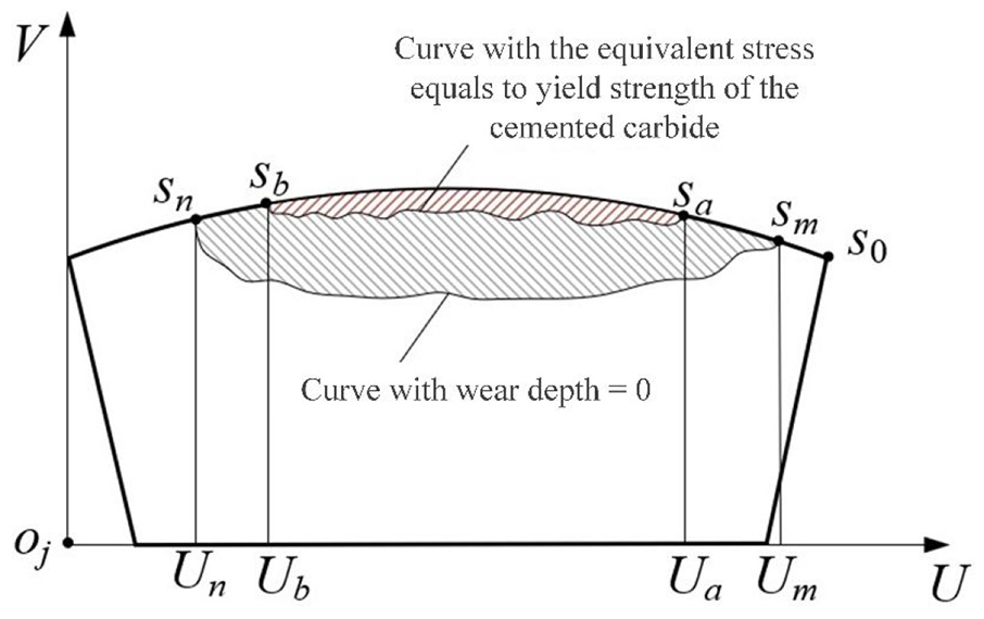
The upper and lower boundaries of the tool blades wear area were examined using a detecting method illustrated in Figure 18. The stress curve equivalent to the yield strength of the cemented carbide was treated as the upper boundary of the tool wear area, while the curve with a wear depth of zero was treated as the lower boundary of the tool wear area.

In Figure 18, o_j-UV is the coordinate system of the wear boundary measurement of the milling tool blades, o_j is the projection of the unworn tip on the mounting surface of the blade bottom, and the U axis is the tangential direction along the midpoint of the cutting edge. The V-axis direction is through the normal point of the tool tip and along the midpoint of the cutting edge, s₀ is the jth tip of the milling tool blade, and s_m and s_n are the two intersections of the lower boundary curve and the cutting edge curve of the jth blade of the milling tool, respectively. s_a and s_b are the two intersections of the upper boundary curve and the cutting edge of the jth blade of the milling tool, respectively. U_n, U_b, U_a, and U_m are the coordinates of the reference points s_n, s_b, s_a, and s_m in the U-axis direction, respectively.

The upper and lower boundaries of the wear area of three tool blades were examined using the detecting method described above, as shown in Figure 19.

Figure 19.

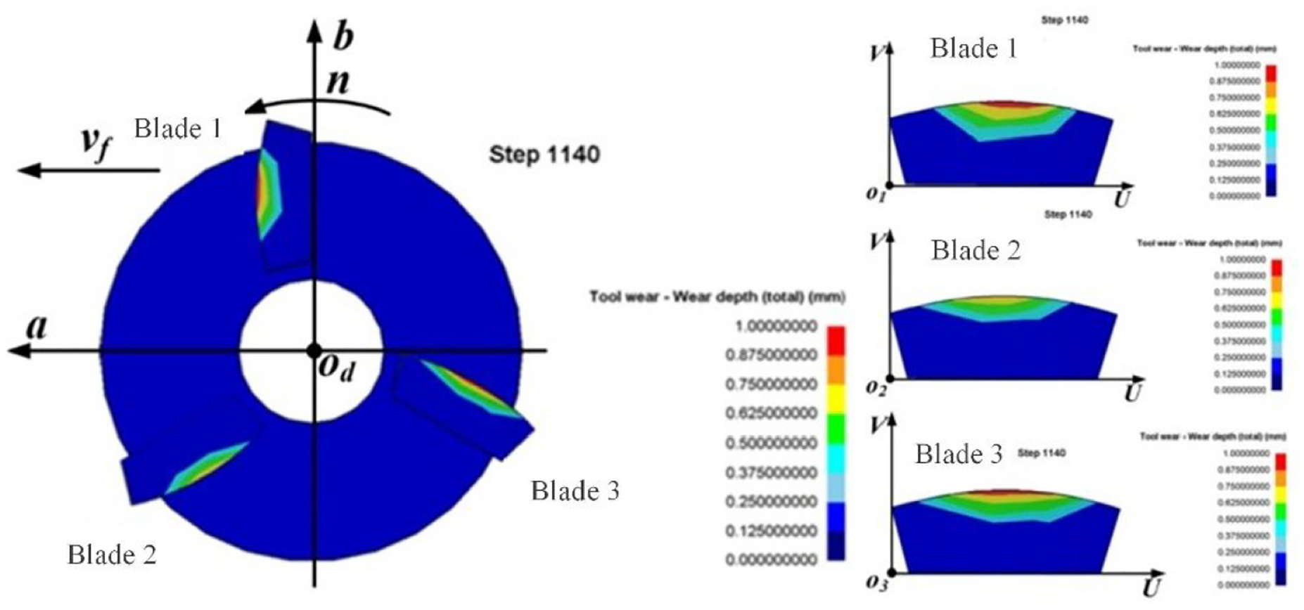
Wear distribution on three blades.

It can be seen from Figure 19 that there was an obvious difference for the wear distributions and values of the three blades. Based on the simulation results described above, it was believed that the differences in the temperatures, stresses, and wear distributions could be acquired using the reconstructed workpiece model, which also meant that the proposed models could efficiently take the influence factors into the dynamic milling process. However, in order to specifically validate the differences, actual milling experiments had to be carried out.

Experimental validation of the differential tool wear models

In order to validate the proposed analytical models, high-feed milling experiments for titanium alloy material were carried out using the same experimental setup described in section “Introduction” and the same milling parameters described in section “Effect of vibration on the instantaneous tool posture and working angle (Level 1–Level 2).” In order to correctly verify the wear distribution of each tool blade, the measurement methods for the wear distribution of the simulation results were the same as those of the experimental results. The measurement coordinate setup of the wear distribution of the simulation results is shown in Figure 20.

Figure 20.

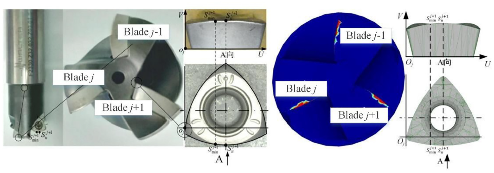
Measurement coordinate setup of wear distribution of simulation results.

Using the above measurement method, the upper and lower boundaries curves of the wear areas in both the simulation and the experimental results were obtained. Figure 21 shows the comparison of the experimental and simulation results for blades 1−3.

Figure 21.

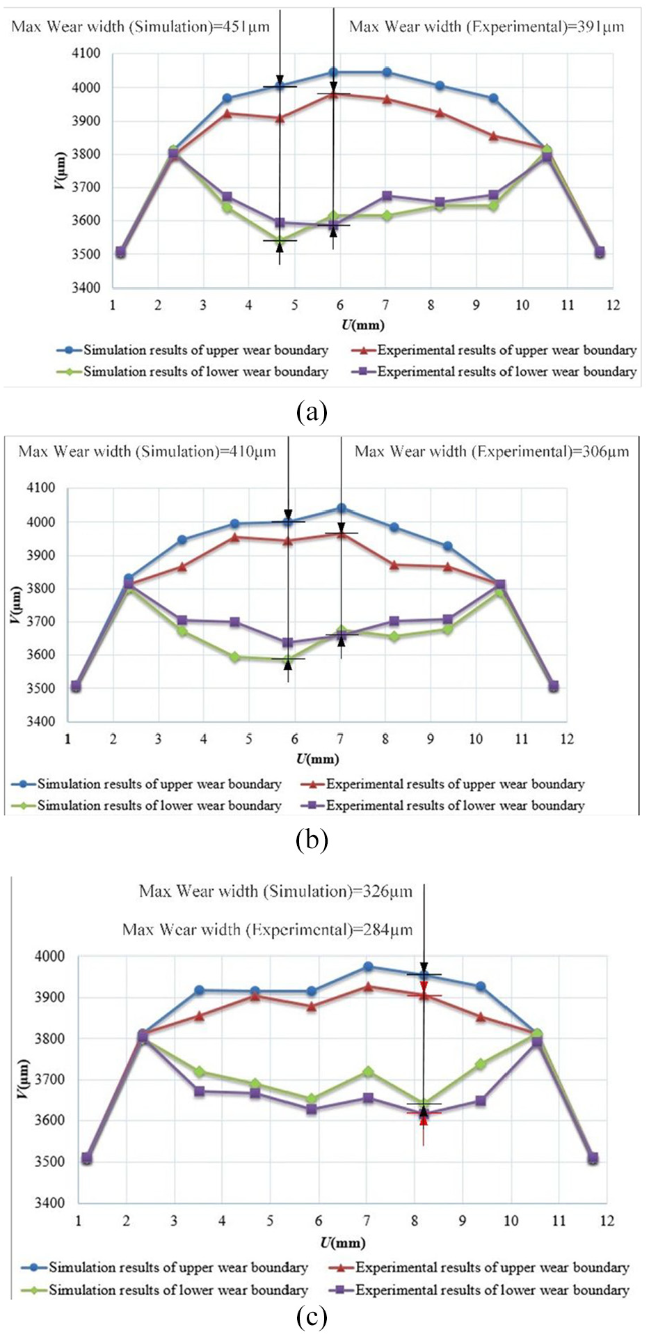
Comparison of experimental and simulation results of the tool insert blades (all the three figures are revised): (a) comparison of experimental and simulation results of blade 1 (L = 0.5 m), (b) comparison of experimental and simulation results of blade 2 (L = 0.5 m), and (c) comparison of experimental and simulation results of blade 3 (L = 0.5 m).

It can be seen from Figure 21 that there were obvious differences in both the maximum wear degree (see Figure 21) and its position, and the wear distributions of the three blades were very different. By comparing the experimental and simulation results, it could also be seen that the simulation and the experimental results showed the similar changing trends for both the upper and lower wear boundaries. The matching degree of the changing trend of the upper wear boundary was better than that of the lower wear boundary. However, the relative errors of the wear values of the upper wear boundary were bigger, which mean that for the wear degree of the cutting edge, the experimental results were more severe. This was probably because there were more possible causes for wear or even micro-chipping in the cutting edge in the actual machining, such as the blade material spalling caused by the shear stresses in flank face, or the cyclical impact between the cutting edge and the workpiece at the cut-in stage. Due to the above reasons, the simulated wear degree of the cutting edge was smaller than that of the experimental results.

Additionally, the maximum wear widths of the three blades in the experiments were 391, 306, and 284 µm, while the values in simulation were 451, 410, and 326 µm. The maximum wear width differences of the blades in the experiments and in the simulation were 107 and 125 µm, respectively. A possible reason for this is that the simulated wear differences of the blades came from the differences of the thermal and stress coupling fields, which were caused by the position errors of the blades and the tool vibration, as described in Figure 9. And the correction of the tool trajectory in simulation was fully based on the vibration data acquired from experiments. However, in the actual machining, the position deviation of the blades was smaller due to the high-frequency interference signals. Thus, the difference in the position errors and corresponding thermal and stress coupling fields between the blades was not obvious compared with that in simulation.

By comparing the obtained wear difference results, the relative error could be calculated as 16.8%. It was believed that the proposed analytical differential wear models could efficiently describe the effect of the milling vibration and the initial errors of the milling tool blades on the differential wear distribution.

Conclusion

In this study, an innovative investigation of the modeling and analysis of differential tool wear in high-feed milling is presented, with a focus on a holistic scientific understanding of the key factors affecting the tool blade wear in the process, further supported by well-designed milling simulations and experiments. Some robust conclusions were drawn as follows:

1. The experimental results for high-feed milling showed that the dynamic deviation from the design of the milling tool postures and working angle caused milling vibrations and initial blades errors, which were the main factors that resulted in the differential thermal stress coupling fields and wear distributions.

2. The differential tool wear models were clearly able to describe the effects of the vibrations and the initial blade errors on the milling tool postures and working angle and able to reveal the influences of the non-linear increases of the contact depths of the tool blades and non-effective cutting times on the distribution of the thermal stress coupling fields.

3. The simulation results showed that the differences in the tool wear, cutting temperatures, and stresses distributions could be simulated using the reconstructed workpiece model and dynamic milling tool postures.

4. The comparison of the experimental and simulation results showed that both results had similar changing trends for the tool wear boundaries, and the relative error of maximum wear width differences of the blades is 16.8%; the differential tool wear models could effectively describe the effects of the milling vibrations and the initial milling tool blade errors on the differential wear distributions.