
Abstract
Due to high stiffness and quick response, dual-drive feed machines (DDFMs) are widely used in many precision CNC machines. The tracking errors of the two feed drives directly determine the machines’ accuracy. The performance of the position accuracy can be easily affected by the difference in the friction dynamic characteristics of the two axes. This paper proposes the state-dependent friction compensation (SFC) as an improved DDFMs error compensation method that can achieve better accuracy under unequal friction on the two feed drives. It is theoretically analyzed the influence of friction on the transmission stiffness of DDFMs. Moreover, the effects of time-varying factors (feed rates and mechanical structures) on the friction of dual axes are discussed. The innovation of the paper is that the SFC can adaptively take into account the influence of the variable dual-drive structure and feed rate on DDFMs’ position accuracy, and the compensation method combined with cross-coupled strategy is suitable for general dual-drive structure. Simulation and experiment results show that the proposed method can effectively improve the synchronization accuracy and tracking accuracy in a variety of feed operations (different feed rates, starting, and reversing).
Keywords
Introduction
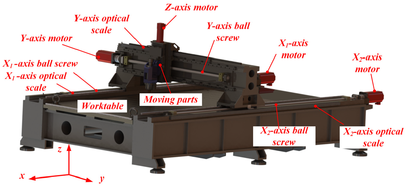
Compared to the traditional single-drive system using a single motor and single ball-screw, the dual-drive feed machines (DDFMs) use dual feed drives and have the advantages of high transmission stiffness and quick response. The DDFMs are built using the principle of Drive at the Center of Gravity (DCG) and are critical to the next generation precision CNC equipment and Cartesian robots.1,2 Figure 1(a) gives an example of the DDFMs; Figure 1(b) shows the DDFMs’ typical structure. The crossbeam (that moves in X1-axis and X2-axis) is driven by a mechanical system containing dual servo motors, dual ball-screws, dual linear guides and bearings. The crossbeam serves as a base of the Y-axis motor. The movement of moving parts driven by the Y-axis motor on the crossbeam causes the loads on the two drives to be different. This variation makes it difficult to directly employ the principle of the DCG in the moving process, as shown in Figure 1(c) and (d).
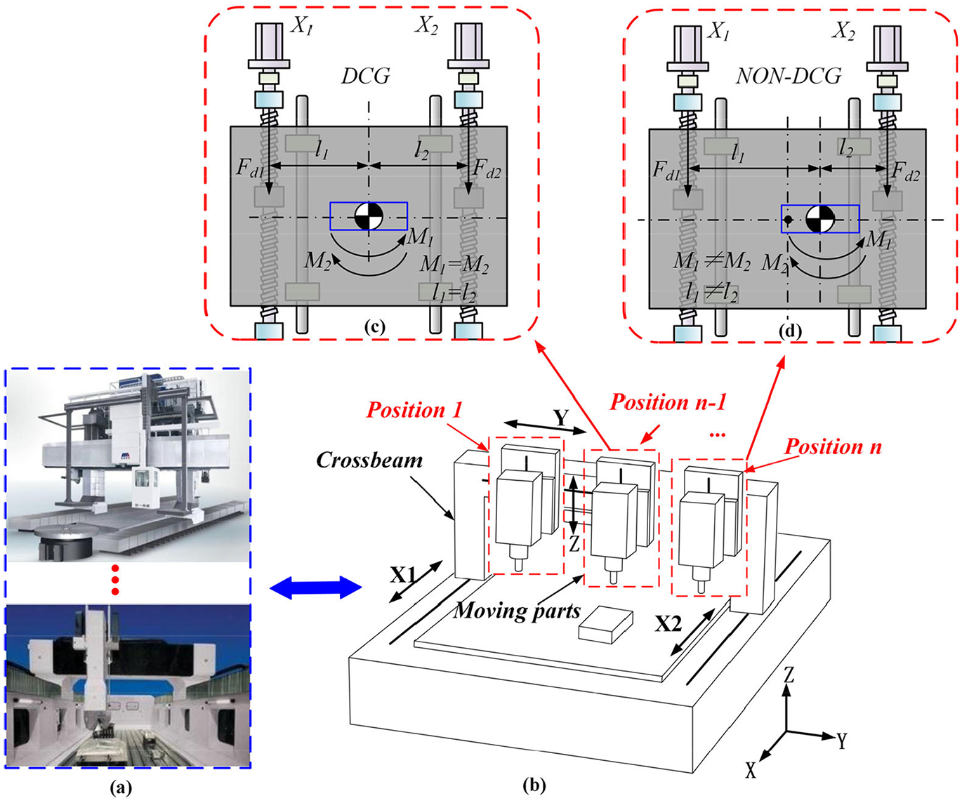
Industrial application of the DDFMs: (a) Gantry-type machine tools (SMTCL CO., LTD. and Zimmermann CO., LTD.), (b) a typical structure of the DDFMs, (c) the principle of the drive at center of gravity (DCG), and (d) the principle of non-drive at center of gravity (NON-DCG).
The moving parts on the crossbeam can also cause friction conditions in the two feed drives to be different. The feed rate of the DDFMs is another proved factor that can affect the friction conditions to change.3,4 The existence of friction may cause stick-slip, limit-cycle oscillation, and steady-state errors. 5 Moreover, friction can influence the transmission stiffness of the DDFMs, and cause the tracking errors 6 (which refers to the position lag between the position command and actual axis positions, as shown in Figure 2(a)) and non-synchronization error (The definition of non-synchronization errors is the difference between X1-axis actual position and X2-axis actual position, as shown in Figure 2(b)) of the two drives. Eventually, the position accuracy of DDFMs can be destroyed. Furthermore, the complex dynamic characteristics of the feed system in combination with unknown friction conditions make accurate feed control even more difficult. 7
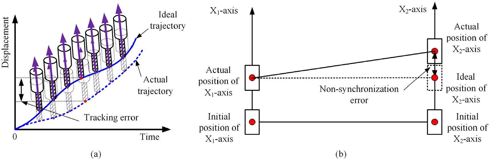
The explanation of tracking error and non-synchronization error: (a) tracking error of the DDFMs and(b) non-synchronization error of the DDFMs.
At present, there are two approaches to compensate for friction in motion control: friction-model based and friction-model free based compensation methods. 8 The friction-model free based compensation method regards friction as an external interference and eliminates it by directly improving the robustness of the control system. 9 This approach may compensate for nonlinear friction if the compensation methods are integrated with learning control, intelligent control, and adaptive control. 10 For example, the nonlinear integral sliding mode control strategy can be applied to the permanent-magnet synchronous motor control system to improve the robustness and dynamic response of the two-axis turntable system by considering the adverse effect of friction and other types of nonlinear disturbances. 11 On the other hand, the merit of friction-model based compensation techniques is that it can directly avoid causing significant friction in the motion of feed drive because it can predict the change of friction and compensate it in advance. Simultaneously, it has strong robustness and simple operation for industrial applications. 12
Generally, two common friction models can be adopted: the static friction model (i.e. Stribeck friction model) and dynamic friction model (i.e. LuGre friction model) to study the friction problems of feed transmission using ball-screw and nuts. Stribeck friction model can well represent friction behavior at low velocities, and parameter identification is convenient. 13 The Stribeck friction model contains Coulomb friction force which accounts for a large portion of the total friction of the feed system is not constant due to different loads on the two feed drives.14,15 LuGre friction model can effectively illustrate the friction characteristics of the pre-sliding regimes and friction memory. Lee et al. 16 adopted the LuGre model to study the friction between ball screws and linear motion guides, and designed an observer-based friction compensation proportional differential position controller for position control. However, the research on friction compensation of the DDFMs is rare in the literature. Owing to the coupling of mechanical characteristics between two axes, friction compensation of DDFMs is more complex than that of a typical single-drive feed drive system. Moreover, there are few studies considering the impact of variation of dual-drive structure (as shown in Figure 1(b)) on the friction of DDFMs. The variation of dual-drive structure generates the difference of two axes’ friction forces, so it is necessary to consider the overall friction force of the system to improve the performance accuracy of the DDFMs.
The DDFMs’ position accuracy also depends on the synchronous control method. An excellent synchronous control method can reduce the feeding error of DDFMs. Common synchronous control methods for the DDFMs include master-slave control, virtual electronic shaft control, and cross-coupled control. Because the core of master-slave control and virtual electronic shaft control is that the master shaft signal is transmitted to the slave shaft, causing the delay of the slave shaft input, so when the system is suffered disturbance or load fluctuation, the non-synchronization errors generated by this method will not be eliminated with the change of time, and it is easy to cause oscillation in the feed system, or even damage the feed system. 17 The cross-coupled control method, proposed by Koren, 18 focuses on the synchronization errors caused by the coupling between the two feed drive systems. This is an integrated strategy that can compensate for motion errors by measuring the position and speed of the two axes and use the obtained data to build a feedback loop. Compared to the master-slave control method, the cross-coupled control method avoids input delays and enables the measurement of disturbance, and therefore usually delivers a better control performance. 19 The mentioned control methods can be combined with some advanced algorithms to build a variety of synchronization control methods, such as the DSP-based cross-coupled intelligent complementary sliding mode method. 20
However, there are a few critical factors, which can affect DDFMs position accuracy, are rarely analyzed simultaneously in the literature.
Due to the flexibility and vibration of the feed drive system, 21 there is a complex mechanical coupling of the dual axes in the case of using ball-screw and nut in the feed transmission system.
The gravity center will be changing when the structure of the DDFMs diversity, as in Figure 1(b), which results in the different friction of two axes and a mismatched disturbance in the system.
Because of the particular structure of DDFMs, a good synchronous control strategy is an important way to improving its performance. Synchronous control strategy should be considered in friction compensation of dual axes.
This research aims to study the state-dependent friction in the dual feed systems and proposes a method that can effectively compensate the state-dependent friction to increase the position accuracy of the DDFMs. The paper reports a new method: state-dependent friction compensation (SFC). The core and novelty are: (1) to analyze the influence of crossbeam feed rate and the positions of the moving parts at the crossbeam, on the friction conditions of the two drive systems, and based on the inner sensor of the motor, identify the friction model of the feed drive system and (2) combined the dynamic characteristic of DDFMs and cross-coupled control strategy, the problem of the tracking errors and non-synchronization errors caused by friction diversity of two axes are solved.
The organization of the rest is as follows. In section 2, the general dynamic model considering the influence of friction is introduced. In section 3, the state-dependent friction model is deduced. Section 4 gives a case study. Finally, the conclusion is shown in section 5.
A general dynamic model of the DDFMs considering the influence of friction
A large number of studies have shown that component kinematic joins of machine tools can greatly affect the dynamics of feed drive system – about 50% static stiffness of a machine tool depends on the stiffness of joints, and more than 90% of the overall damping performance is determined by joints.22,23 Therefore, the research focus of mechanical analysis should be on the kinematic stiffness of the ball-screw and nut joints. Furthermore, the transmission stiffness of the feed system is smaller when compared to that of other directions,24,25 so the stiffness of the transmission direction is considered in this paper. Figure 3 shows the dynamic model of the DDFMs.
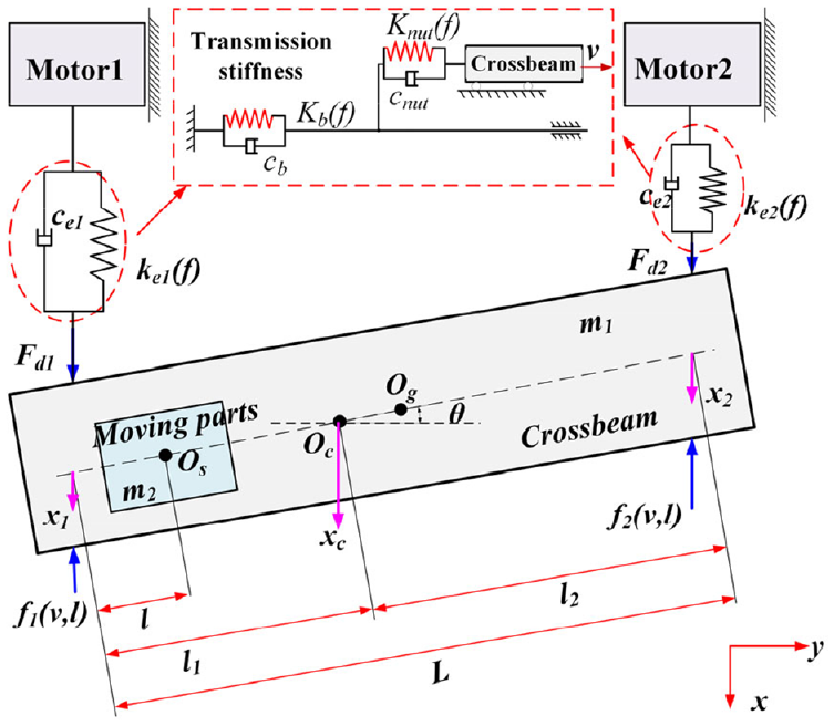
The dynamic model of the DDFMs.
The ball-screw and nut joints and bearing joints can be represented by lumped spring elements, and the crossbeam can be seen as a lumped mass element. Figure 3 clearly shows that the transmission stiffness of the single feed drive is determined by ball-screw and nut contact stiffness and ball-screw and bearing contact stiffness.
In Figure 3, ke1(f) and ke2(f) are the transmission stiffness of the feed system on the X1-axis and X2-axis, respectively. The subscript (f) indicates that the transmission stiffness is a function of the friction f. Knut(f) and Kb(f) are axial contact stiffness between the ball-screw and nuts, and axial contact stiffness between the ball-screw and bearing, respectively. ce1 and ce2 are equivalent dampings of the X1-axis and X2-axis, respectively. cnut and cb are the damping of ball screw nut joint and bearing joint, respectively. Og and Os are the center of gravity of the crossbeam and the moving parts on the crossbeam, respectively. Oc is the center of gravity of the combined body, which contains the crossbeam and the moving parts. l1 is the distance between Oc and X1-axis; l is the distance between Os and X1-axis; l2 is the distance between the Oc and X2-axis. L is the length of the crossbeam. Owing to different tracking errors between X1-axis and X2-axis, the crossbeam has a rotation angle θ in the process of movement which is caused by the different friction on the two axes. f1(v,l) and f2(v,l) are the friction forces on X1-axis and X2-axis, respectively, both of them are the function of feed rate v and moving parts position l. m1 and m2 are the mass of crossbeam and the moving parts, respectively. xc is the displacement of Oc. x1 and x2 are the actual displacements of the two axes, respectively.
During the movement of the DDFMs, because of the different forces on dual axes, the mechanical difference between X1-axis and X2-axis can cause non-synchronization errors. Considering axial displacement of X1-axis and X2-axis, and rotation angle of the crossbeam, the dynamic equations are in equation (1).
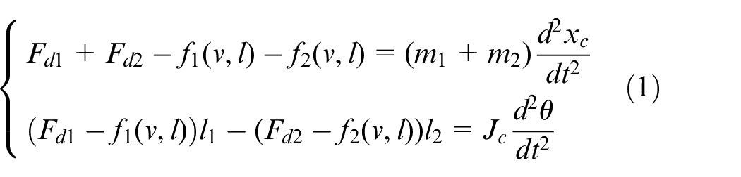
where Fd1 and Fd2 are the axial driving forces in X1-axis and X2-axis, respectively. Jc is the rotary inertia of the overall load around Oc.
The relation of J1, Jc, and J2 can be expressed as in equation (2).
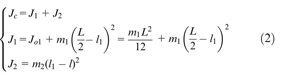
where Jo1 is the moment of the crossbeam around Og; J1 and J2 are the rotary inertia of the crossbeam and the moving parts around Oc, respectively.
The relation of axial equivalent stiffness and axial driving forces can be given as in equation (3).
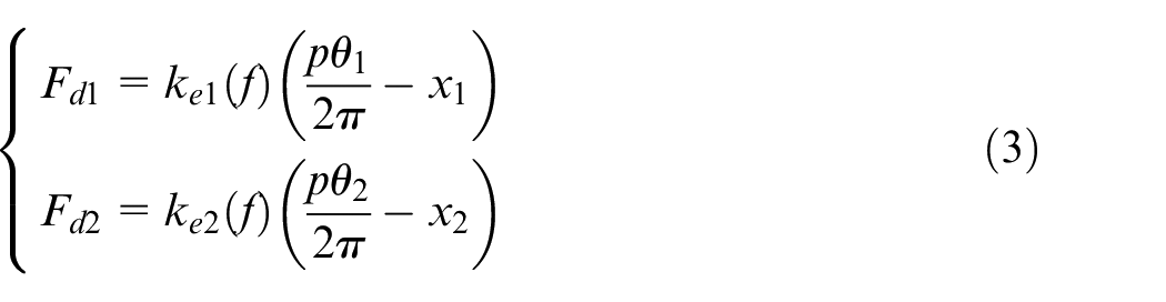
where p is the lead of the ball-screw, θ1 and θ2 are the X1-axis and X2-axis motor output angles, respectively.
According to the stiffness series equation, 26 ke1(f) and ke2(f) are given in equation (4).
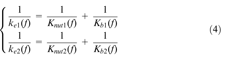
where Knut1(f) is axial contact stiffness between the X1-axis ball-screw and nuts. Knut2(f) is axial contact stiffness between the X2-axis ball-screw and nuts. Kb1(f) is the axial contact stiffness between the X1-axis ball-screw and bearings. Kb2(f) is the axial contact stiffness between the X2-axis ball-screw and bearings. Hertz contact theory can be adopted to calculate Kb1(f), Kb2(f), Knut1(f), and Knut2(f). The (f) means that they are the function of friction. The specific calculation formulas can be referenced to Lu et al. 27
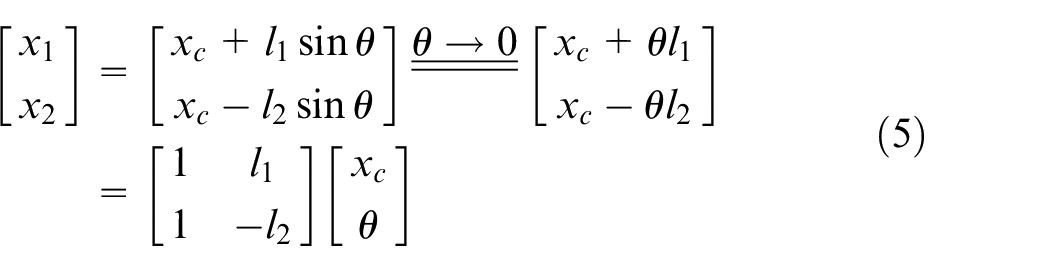
According to the geometric relationship described in Figure 3, the relationship of x1, x2, and xc is as follows in equation (5).
Substitute equations (2), (3), and (5) into equation (1), then take the Laplace transform of the new equation, to yield equations (6)–(8).
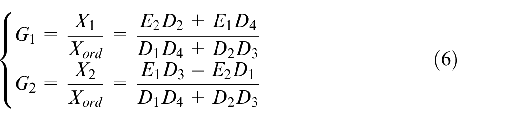
where G1 and G2 represent the transfer function of X1-axis and X2-axis respectively. Xord is X1-axis and X2-axis motor command of output position, X1 and X2 are the actual output of X1-axis and X2-axis respectively.
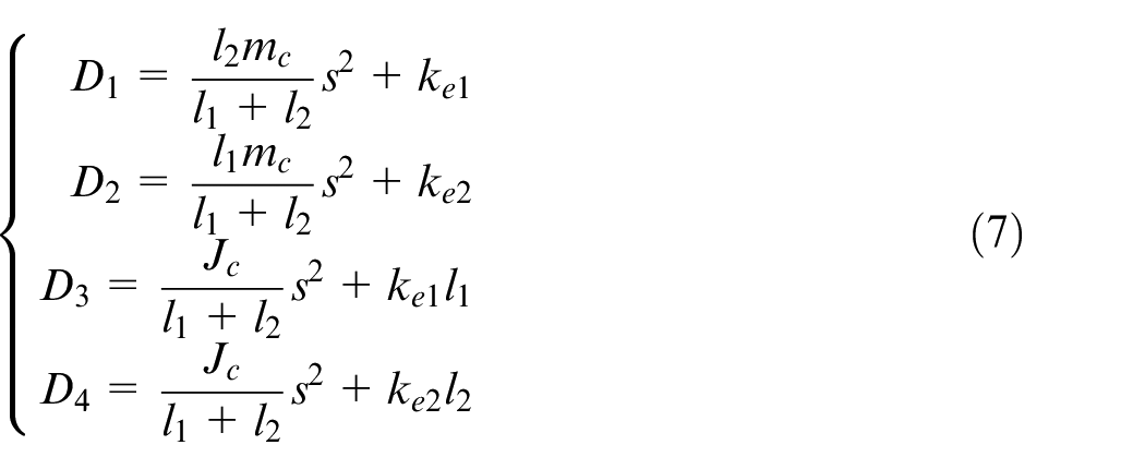
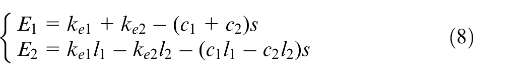
where c1 and c2 are coefficients of the X1-axis and X2-axis friction force. mc is the mass of the overall load, and its expression is mc = m1 + m2.
State-dependent friction model of DDFMs
In the process of moving, the moving parts move on the crossbeam, resulting in time-varying structure of DDFMs. The moving parts near either end of the crossbeam would change the loads on the two axes. Figure 4 shows the effects of different positions of the moving parts on the forces on the X1-axis and X2-axis.
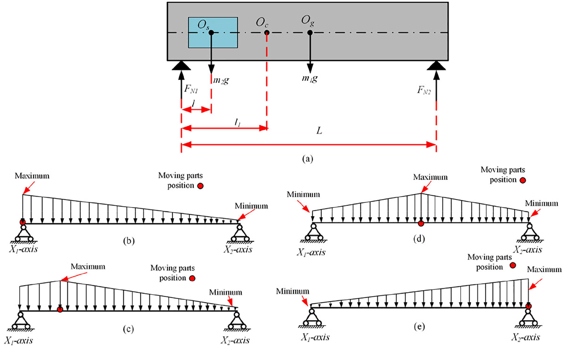
Crossbeam forces analysis diagram. (a) The vertical forces of the crossbeam and moving parts (b–e) Show force analysis at the different positions of moving parts.
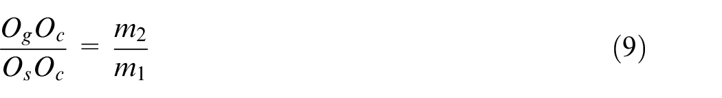
It can be seen that the relationship of Oc, Og, and Os can be written as in equation (9).
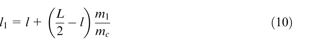
Therefore, the l1 can be expressed as in equation (10).
According to the principle of forces and moments balance, equation (11) can be obtained.
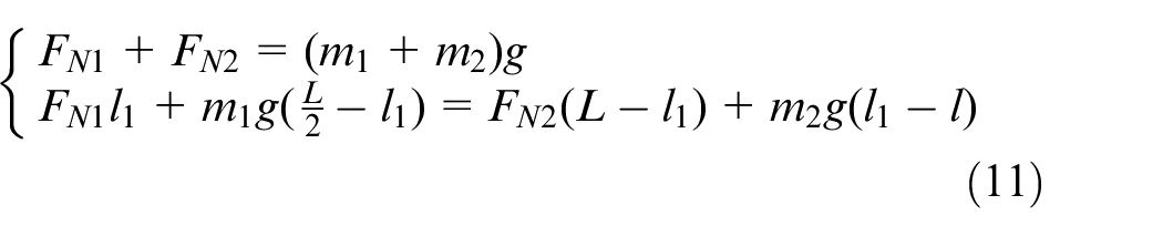
where FN1 and FN2 are the support forces of the X1-axis and X2-axis. Equation (11) can be simplified to yield equation (12).
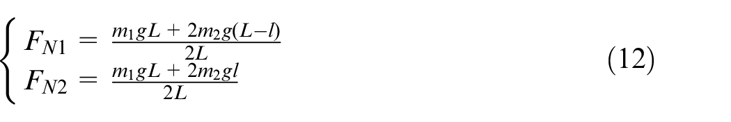
It can be seen from equation (12) that the change of l can alter the normal force on the two axes, and thus change the friction forces. The Stribeck friction model combines the characteristics of static friction, kinetic friction, and viscous friction model. The maximum static friction, viscous friction coefficient, and Stribeck velocity are not simply linearly related to position l, and it is a relatively comprehensive model of the real friction phenomenon and can show the non-linear and negative slope characteristics in the low-velocity regions. Therefore, this study uses the Stribeck friction model to analyze the effects of the feed rate of the crossbeam and the different positions of the moving parts on the friction along the two axes.
Parameter identification of state-dependent friction model
The relevant parameters in the Stribeck friction model can be obtained using the genetic algorithm (GA).23,28 Then, the relationship between the position of the moving parts and the frictions on X1-axis and X2-axis can be built using the Newton interpolation method. 29 Finally, the relationship function of friction, feed rates, and the positions of the moving parts can be derived. The parameter identification process of the friction forces model is shown in Figure 5.
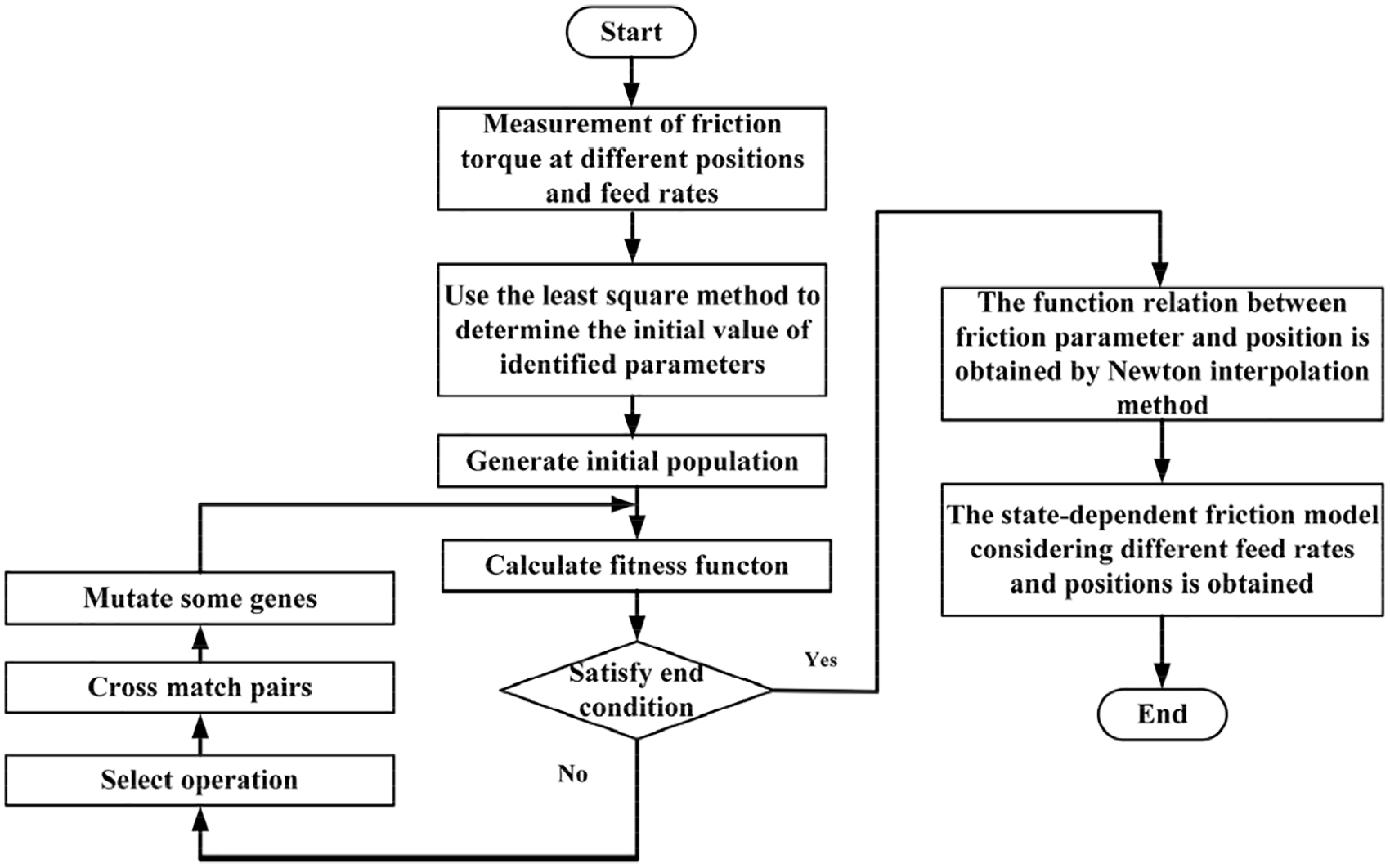
The parameter identification process of the state-dependent friction model.
The expression of the Stribeck friction model is in equation (13). 30
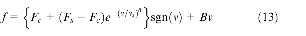
where Fc is kinetic friction; Fs is static friction; vs is Stribeck velocity; B is the viscous friction coefficient.
The friction torque is usually used in the identification process, and thus the Stribeck friction model can be modified as in equation (14).
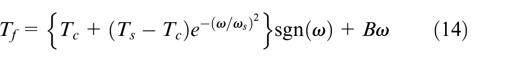
where Tc is the kinetic friction torque; Ts is the static friction torque;
In the process of friction identification, when the crossbeam moves at a constant feed rate, where there are no torques caused by accelerations, the friction torque Tf and the driving torque Td have the relationship as in equation (15).
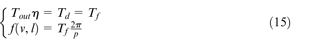
where η is the output efficiency of the motor rated torque; Tout is the output torque of the motors; f(v,l) is the friction force of the feed drive system, the (v,l) means that friction is function of v and l.
The parameters in the Stribeck friction model can then be identified after measuring the friction torques via experiments. The least-square method is used to determine the initial value of the parameters Tc, Ts, vs, and B, and then the GA is adopted to improve the accuracy of parameter identification. The least-square method is suitable for linear as well as nonlinear systems, due to its relatively simple computational process. GA can solve complex optimization problems in many fields and the GA method’s global optimization performance has been widely acknowledged.23,28 The initial values can be given by the least-square method, and the GA can help refine the results. These two methods are combined so as to build an overall accurate and quick parameter identification process.
As shown in Figure 5, the key steps of the GA are as follows:
Optimization variables. Set the parameters Tc, Ts, vs, and B are the optimization variables. It can be defined as that
Fitness function. The fitness function is to calculate the fitness value and evaluate individuals’ excellence. The closer the identification result is to the measurement value, the better the effect will be. So it can be defined as follows:
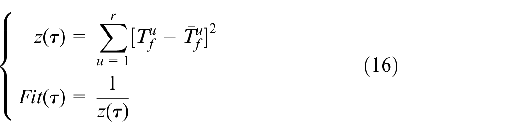
where
Key parameters setting. The chromosome encoding method is double precision real number coding, which can improve search efficiency and accuracy. The stop condition adopts the biggest evolution iteration.
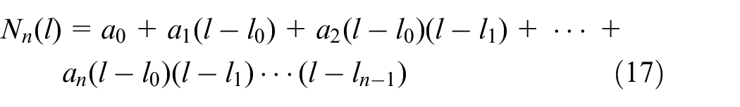
To understand the influence of the moving parts position on the friction, Tc, Ts, vs, and B can be regarded as a function of l. Tc(l), Ts(l), vs(l), and B(l) functions can be obtained using the Newton interpolation method, which is a straightforward fitting method and can be expanded easily. 29
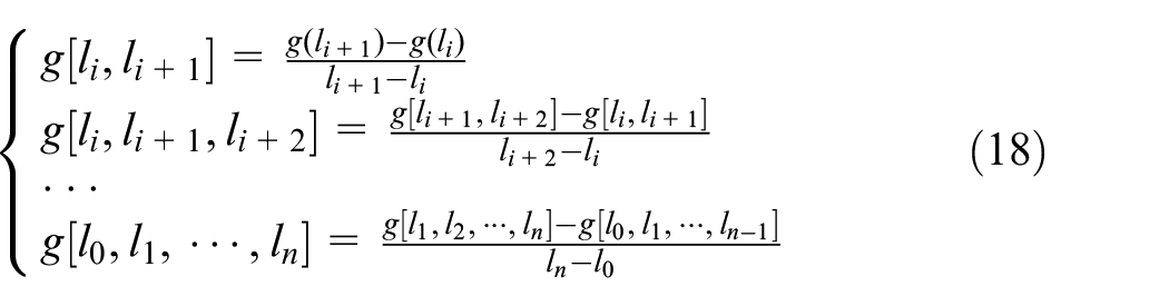
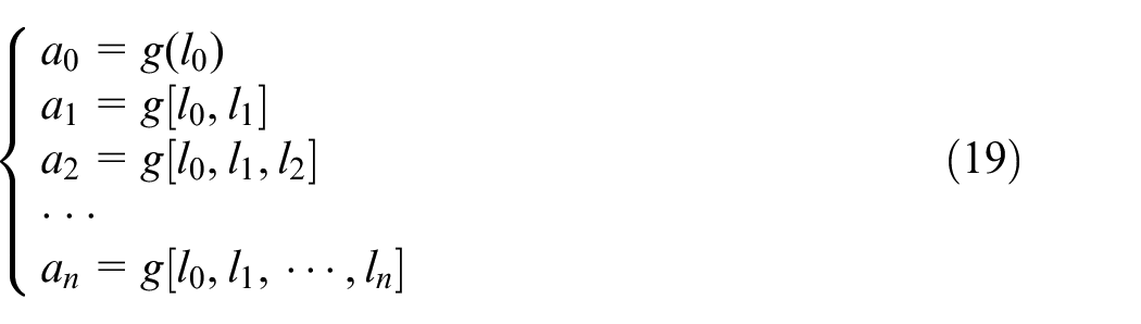
Suppose Nn(l) is the nth-order Newton interpolation polynomial, it can be expressed as in equation (17). In the process of parameter identification, Nn(l) represents Tc(l), Ts(l), vs(l), and B(l), respectively.
when the moving parts are in different positions, the relevant measure data can be expressed as (li, g(li)) (i = 0,1,…,n).
The state-dependent friction compensation (SFC)
A key principle used in this research is to compensate friction in real-time by increasing the torque in the current loop of the controller, thereby mitigating the effect of friction on the system motion performance. The core of the SFC is proposed by combining the established state-dependent friction model with a cross-coupled control strategy. Specifically, the friction models established in the previous deduction are used to compensate for the dual-axis friction in real-time. Combined with the cross-coupled control method, considering the influence of feed rate and the variation of moving parts position on the dynamic characteristics of the DDFMs, real-time position loop compensation is carried out to reduce the tracking error and non-synchronization error and improve the position accuracy.
The cross-coupled synchronous control (CCSC) method refers to giving the control signal to dual transmission systems, calculating the non-synchronization errors between the dual transmission systems through measurements, and targeting the errors as the control object. The CCSC method considers the coupling relationships of the two axes, and compensates for their position deviations. It is commonly used as a proportional-integral-derivative (PID) controller in the CCSC.
The AC permanent magnet synchronous motor (PMSM) is used in this experiment, and the servo system is controlled by three loops: the motor current loop, velocity loop, and position loop. This PID approach is adopted from Chen et al., 31 and its expression is shown in equation (20).
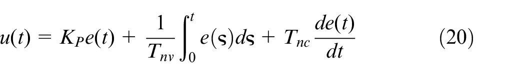
where u(t) is output signal; e(t) is deviation signal; Kp is proportional coefficient; Tnv is the integral time constant; Tnc is the differential time constant.
Figure 6 shows the principle block diagram of the SFC method. According to the mathematical model of the PMSM, 32 classical three-loop control is adopted for the servo system. A proportional (P) controller, which can reduce overshoot and oscillation, is used for the position loop. A proportional-integral (PI) controller, which can ensure good response performance and stability of the velocity loop, is used for the velocity loop, and a PI controller is used for the current loop, which can reduce the influence of the harmonic component generated by the armature electromotive force. Combined with the identified friction model of two axes, the inputs of the friction compensation model are the positions of the moving parts l and feed rates v, and the outputs are the friction torques (Tf1 and Tf2) to be compensated, which is compensated into the servo current loop in real-time. At the same time, combined with the dual-drive dynamic transfer functions G1 and G2, the actual displacements of the X1-axis and X2-axis are finally output. The actual displacements of two axes are fed back to the cross-coupled controller through the linear optical scales on both sides of the machine bed. A proportional and derivative (PD) controller is adopted, which can reduce the lag of cross-coupled control and increase the stability of the system. Therefore, the non-synchronization error signal can be adjusted in the shortest time. β1 and β2 are the feed forward proportional coefficient of the velocity loop. Through the cross-coupled controller, the dual-axis displacement compensation value is output to complete the two-axis synchronous control.
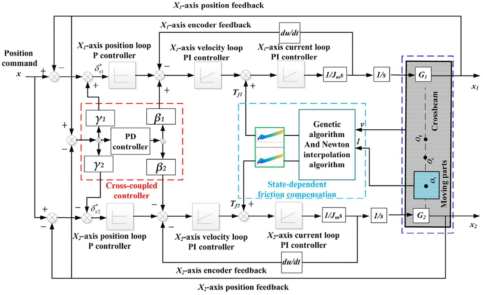
The block diagram of the SFC method.
As shown in Figure 6, x and x12 are the actual displacements of X1-axis and X2-axis respectively, x is the ideal displacement (position command), tracking error and non-synchronization error of the two feed systems are shown in equation (21).
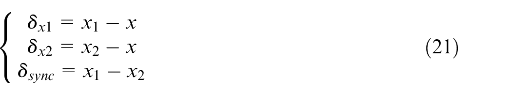
where
To consider the coupling relationship between errors, the tracking error and non-synchronization error are defined as
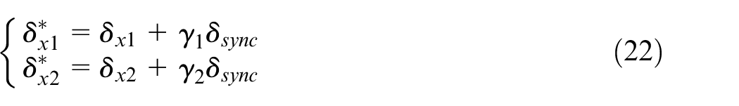
where
A case study: SFC for dual-drive gantry-type machine tool
The dual-drive gantry-type machine tool (DGMT) is chosen as an example to illustrate the performance of the proposed method. The structure of the DGMT is shown in Figure 7; it has three feed directions: X-direction, Y-direction, and Z-direction. X-direction (crossbeam movement direction) adopts the DCG principle. The moving parts, which contain saddle, Z-direction motor and headstock, can move on the crossbeam along the Y-direction, using a singular motor and ball-screw. The X-direction and Y-direction stroke are 2000 and 1200 mm, respectively. When the moving parts move along Y-direction, X1-axis friction forces and X2-axis friction forces will change.
The structure of the dual-drive gantry-type machine tool (DGMT).
Friction model identification experiments
The parameter identification process of the state-dependent friction model is illustrated using the X1-axis as an example, the method and process for the X2-axis are the same. The experiment is shown in Figure 8. A zero value of l indicates that the position of moving parts is near the X1-axis. Under the condition of l = 0, the crossbeam feed rate in the range 200–3000 mm/min was adopted as an example to identify the X1-axis friction model parameters. The output torques of the motors were measured by the internal sensor of the motors. Besides, the empirical mode decomposition (EMD) method was used for data processing.
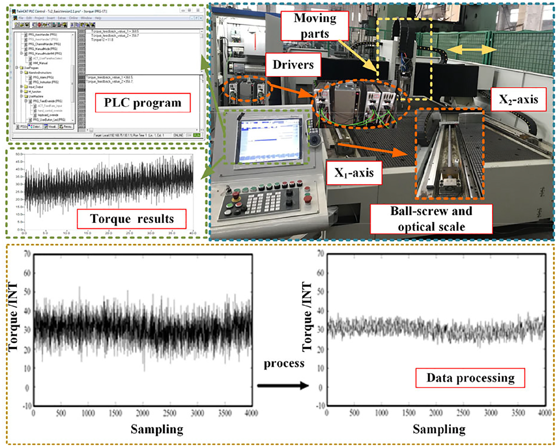
State-dependent friction model identification experimental diagram.
The least-square method was adopted to fit the low-velocity region and the middle-high velocity region using the equations
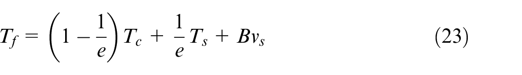
Equation (23) is combined with
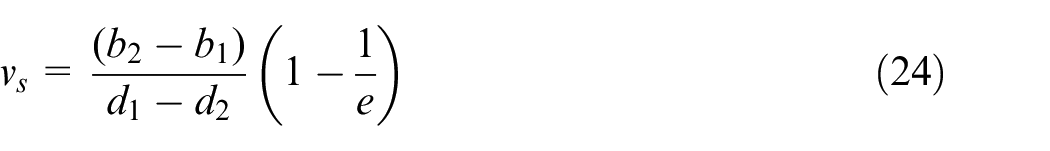
where
The initial value of Tc, Ts, vs, and B can be calculated by equations (23) and (24), these parameter values are 334.99 N mm, 383.07 N mm, 4.32 mm/s and 2.67 mm/s, respectively.
Then, the GA method is used to improve the accuracy of the identified parameters. This can be done using Matlab® by setting the upper bound of
The stroke of the moving parts moving on the crossbeam is in the range from 0 to 1.2 m. Here, l is set to 0, 0.2, 0.4, 0.6, 0.8, 1.0, and 1.2 m in experiments. The parameter identification process is repeated for different l settings, and the relevant parameters of the Stribeck friction model in terms of the X1-axis and X2-axis can be obtained.
Based on equations (14), (15), (17)–(19), the state-dependent friction models of DDFMs can be obtained in equation (25).
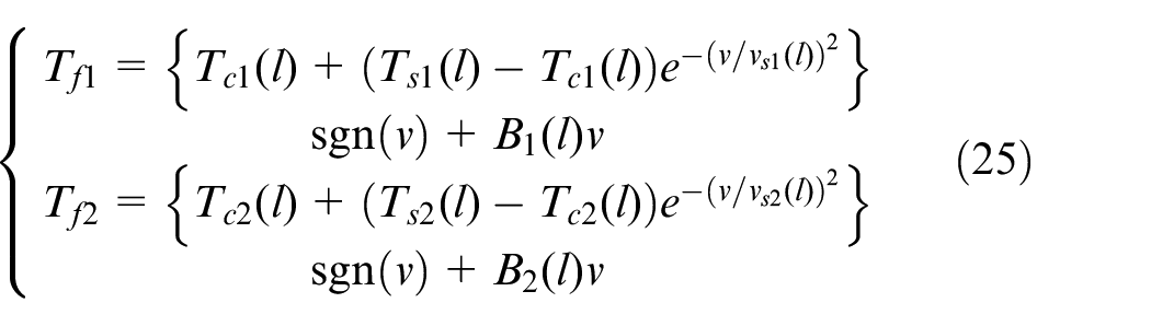
where
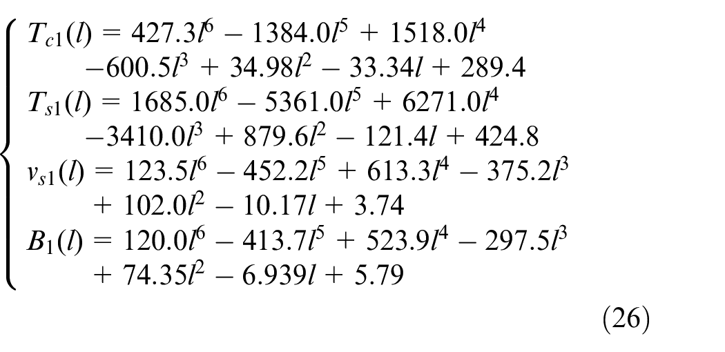
and
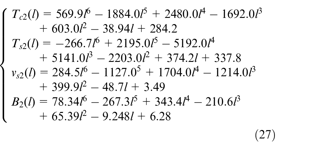
In equations (26) and (27),
Figure 9(a) and (b) show the state-dependent friction models for X1-axis and X2-axis, respectively. It can be seen that the Stribeck phenomenon of the X1-axis is more obvious than that of the X2-axis. This difference is caused by different mechanical characteristics (e.g. servo characteristics and lubrication conditions). An increased l value means that the moving parts shift from the X1-axis side to the X2-axis side – the friction on the X1-axis decreases, and the friction on the X2-axis increases.
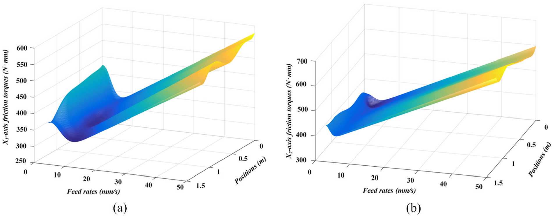
State-dependent friction model for: (a) X1-axis and (b) X2-axis.
The calculation of axial stiffness of the DGMT
Adopting Hertz’s contact theory, the expression of contact stiffness of the feed drive system can be obtained. The calculation formulas are in equation (28). Firstly, the forces of the joint are analyzed to calculate the normal force between the contact bodies, then the sum of synthetic curvature of the contact body is calculated according to the structural parameters. Next, the contact deformation is calculated through the formula, and then the axial deformation is obtained from the geometric relationship, so as to calculate the contact stiffness. Finally, the transmission stiffness of the X1-axis and X2-axis (ke1(f) and ke2(f)) are obtained.
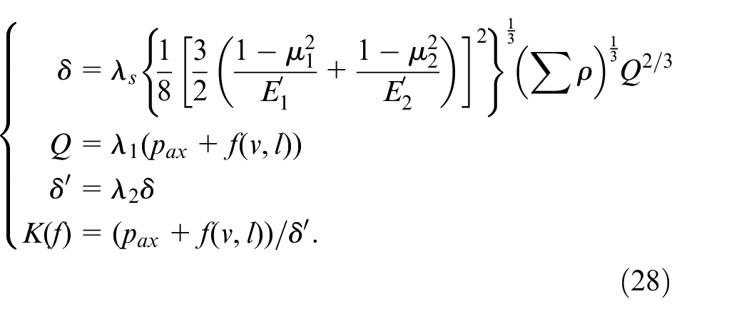
where
Combined with equation (28), ke1(f) and ke2(f) can be calculated by relevant parameters, which can be found in the technical manual shown in Table 1. In Table 1,
The parameters of key joints.
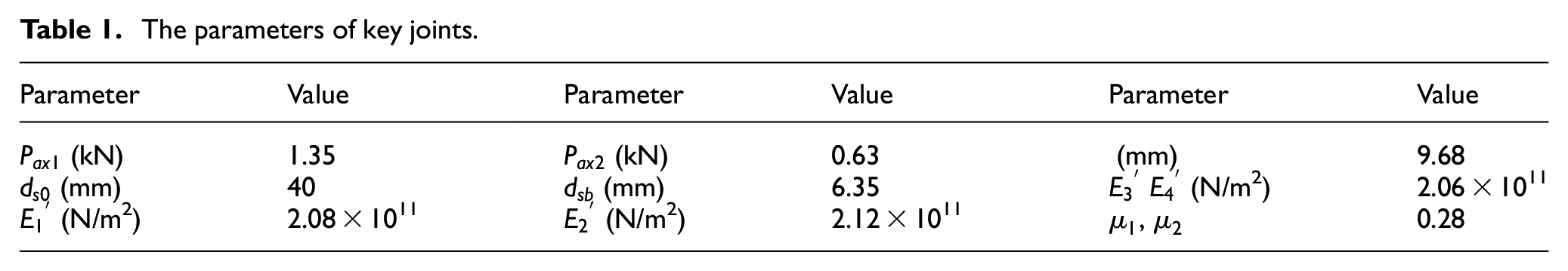
Figure 10 shows the transmission stiffness of the X1-axis and X2-axis. It can be seen that at the same feed rate, the transmission stiffness of the X1-axis and X2-axis are different, even if the moving part is in the middle of the crossbeam, at this moment the dual-drive structure is symmetrical. The results show that diverse friction forces on two axes can cause the transmission stiffness difference between two axes. Moreover, the different transmission stiffness of dual axes is one of the reasons for causing the position error. Therefore, it is necessary to consider the transmission stiffness in the compensation method.
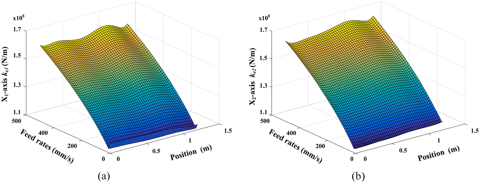
The transmission stiffness ke1 and ke2 of the X1-axis and X2-axis: (a) transmission stiffness of X1-axis and (b) transmission stiffness of X2-axis.
Simulation
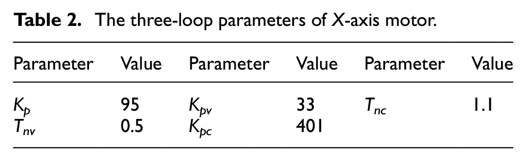
The three-loop parameters of the servo motor need to be adjusted. The setting principle is to make the servo system have good position accuracy, fast response performance, and strong anti-interference ability. According to the regulation of parameters, this paper lists the three-loop parameters of the motor after setting, 33 as shown in Table 2. In Table 2, Kp is the proportional coefficient of the position loop; Kpv and Tnv are the proportional coefficient and integral time constant of the velocity loop, respectively; Kpc and Tnc are the proportional coefficient and differential time constant of the current loop, respectively.
The three-loop parameters of X-axis motor.
As shown in Figure 11, the block diagram of the SFC can be combined with the state-dependent friction model and DDFMs dynamic model. The inputs are the crossbeam feed rate, the position of the moving parts, and X-direction position command. Then, the overall performance of the SFC can be simulated. Gs3(s), Gs2(s), and Gs1(s) are the servo motor transfer function of the position loop, velocity loop, and current loop, respectively. Kig and KT are feedback coefficient and a torque coefficient, respectively. Ki1, Kv1, and Kpp1 denote the current loop feedback coefficient, velocity loop feedback coefficient, and position loop feedback coefficient of servo motor X1-axis, respectively. Ki2, Kv2, and Kpp2 denote the current loop feedback coefficient, velocity loop feedback coefficient, and position loop feedback coefficient of servo motor X2-axis, respectively.
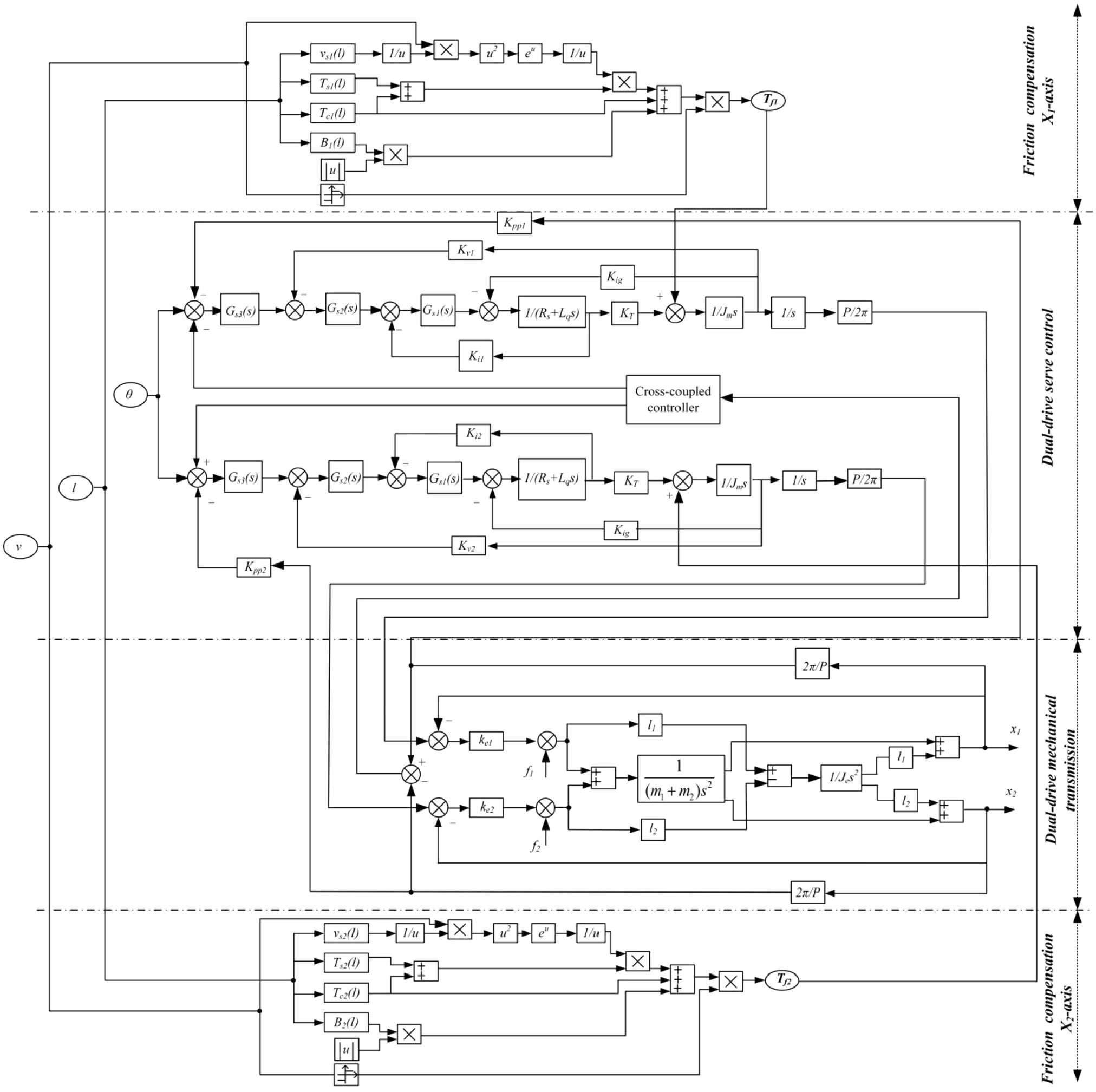
Simulation block diagram of the SFC.
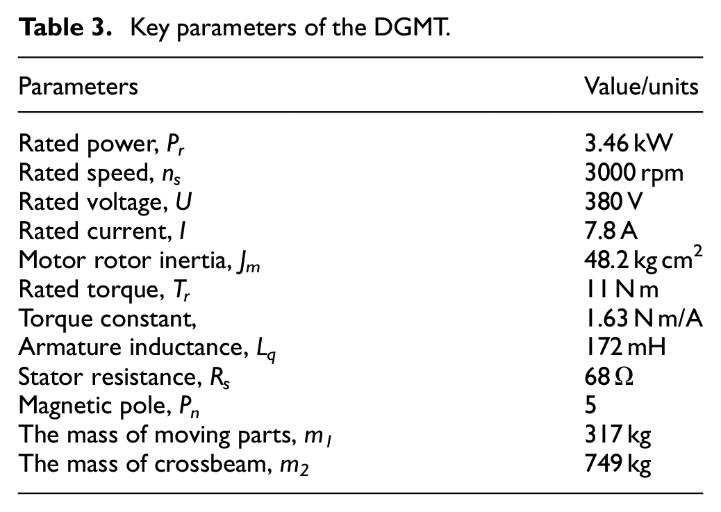
The PMSM parameters and key parameters of the DGMT are used in the simulation. The specification details are shown in Table 3.
Key parameters of the DGMT.
In order to prove that the proposed error compensation method can effectively improve the feed accuracy of the DDFMs, there are two aspects of simulation verification: (1) Verify the response speed, overshoot and anti-interference ability of the proposed method; (2) Verify the tracking accuracy and synchronization accuracy of the system under different positions of the moving parts. The simulation results are compared to that using the CCSC method (using the P controller) under the same conditions. The CCSC method is a common method for dual drive synchronous control.18,19
Verify the response speed, overshoot, and anti-interference ability of the proposed method.
As shown in Figure 12(a), when a step signal with an amplitude of 1 is input to the control system, the single-axis response speed of the SFC is faster than that of the CCSC, and a disturbance is given to the system in 4 s. The error of the single-axis with the SFC is lower than that with the CCSC. Figure 12(b) shows that the non-synchronization error of the SFC method is smaller than that of the CCSC and the recovery rate is faster than that of the CCSC. Simulation results show that the proposed error compensation method has fast response speed and good anti-interference ability.
(2)Verify the tracking accuracy and synchronization accuracy of the system under different positions of the moving parts
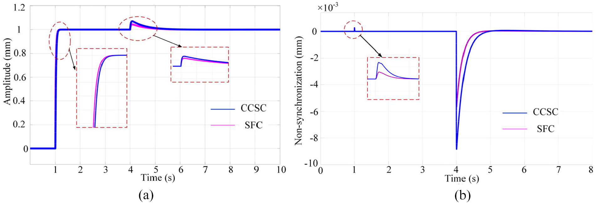
Simulation results of (a) response speed and (b) anti-interference ability comparison between CCSC and SFC.
To verify the effect of the SFC, the moving parts are placed in different positions (i.e. l = 0, l = 0.3 m, l = 0.6 m), and the input ramp signals slopes of 5, 25, and 50 are used. Different ramp signal slopes are used to simulate different feed rates. The X1-axis simulation results under the condition of l = 0 and ramp signal slopes of 5 are given in Figure 13.
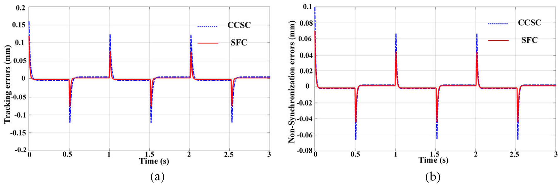
Simulation results of tracking errors (a) and non-synchronization errors (b) comparison between the CCSC and the SFC.
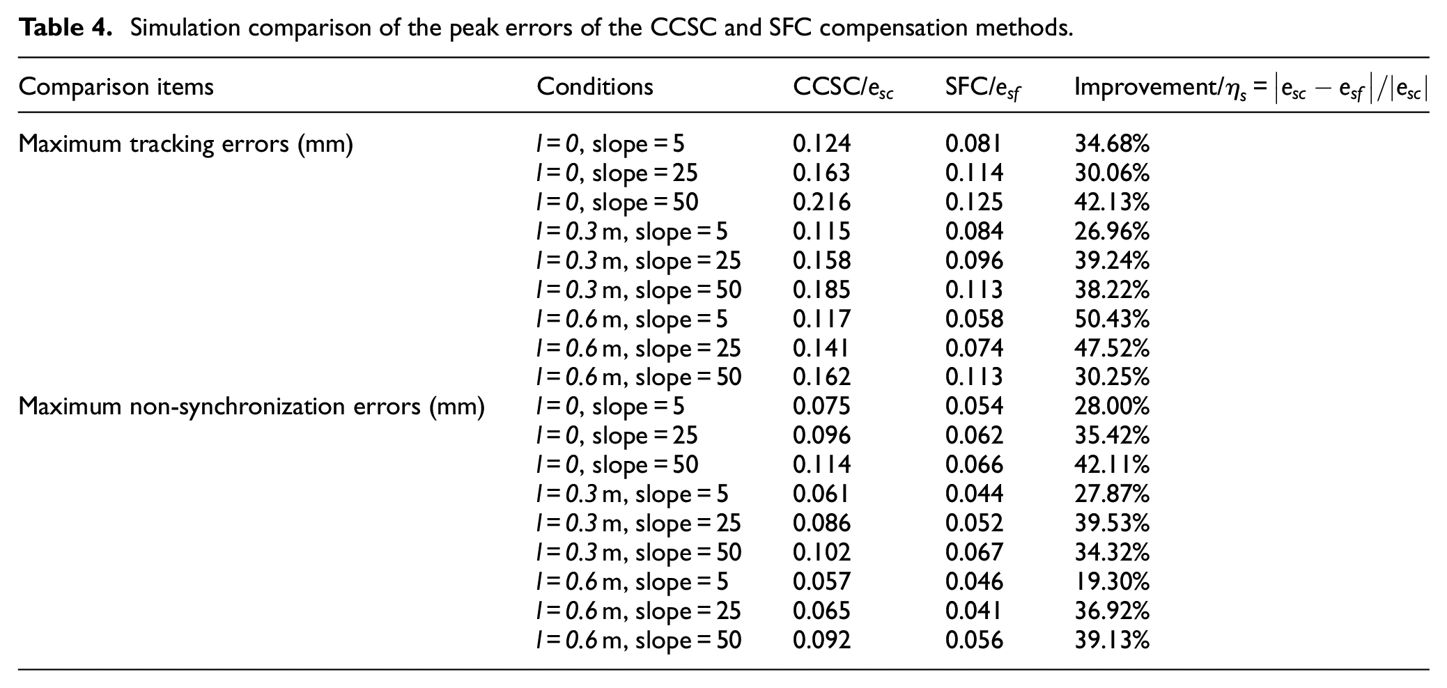
Figure 13(a) and (b) show the tracking errors and non-synchronization errors, respectively, in terms of using CCSC and SFC. It can be seen that when the SFC is not considered (i.e. using CCSC), there are obvious tracking errors and non-synchronization errors. Some steady-state errors are also observable. When the state-dependent friction compensation is considered (i.e. using the proposed SFC), the steady-state position errors, maximum tracking errors, and maximum non-synchronization errors are all reduced. The reduction in the latter two is significant. As shown in Table 4, the reduction in the tracking errors and the non-synchronization errors can reach 50.43% and 42.11%, respectively. The simulation results show that SFC can improve the tracking accuracy and the synchronization accuracy of the DDFMs. Simulations using other input ramp signals give a similar conclusion.
Simulation comparison of the peak errors of the CCSC and SFC compensation methods.
Experimental evaluation
The hardware integration diagram of the DGMT is shown in Figure 14. The control system of the machine tool is constructed using a BECKHOFF system, in which the drivers and motors adopt AX5000 series drivers and AM8500 series AC servo motor, respectively; I/O module adopts the EtherCAT bus terminal module, mainly using EK1100 series, EL1800 series, EL2800 series, and EL5000 series components. The control program is built using TwinCAT3® software. TE1400 project plug-in is included in the BECKHOFF control system and can convert the Matlab®/Simulink model into real-time C/C++ codes through the Simulink coder, and compile the model into the TcCOM module with feasible input-output interfaces, which can be recognized and called by the BECKHOFF system, and can be executed in TwinCAT runtime core online. 34
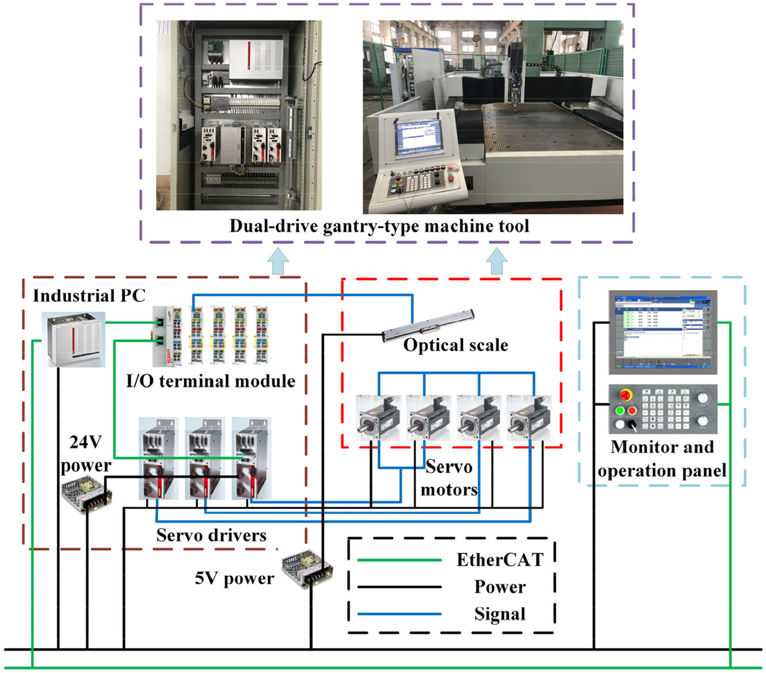
The hardware architecture of the controller for the dual-drive gantry-type machine tool (DGMT).
The controller reads the position feedbacks of the linear optical scales in real-time at a certain sampling frequency, and makes the real-time adjustment to position instructions according to the feedback signal. Figure 15 shows the process of the error compensation experiment. Firstly, using TE1400 to transform the SFC Simulink model (which is shown in Figure 11) into a real-time TcCOM module with its own input and output interface, and then connect the input and output variables of the TcCOM module to the servo system variables. For instance, the compensated torque of the friction compensation can be achieved with increased current by connecting the additional torque instruction interface provided by the current loop in the servo system. Finally, setting some parameters such as cycle period in the servo system to realize the error compensation.
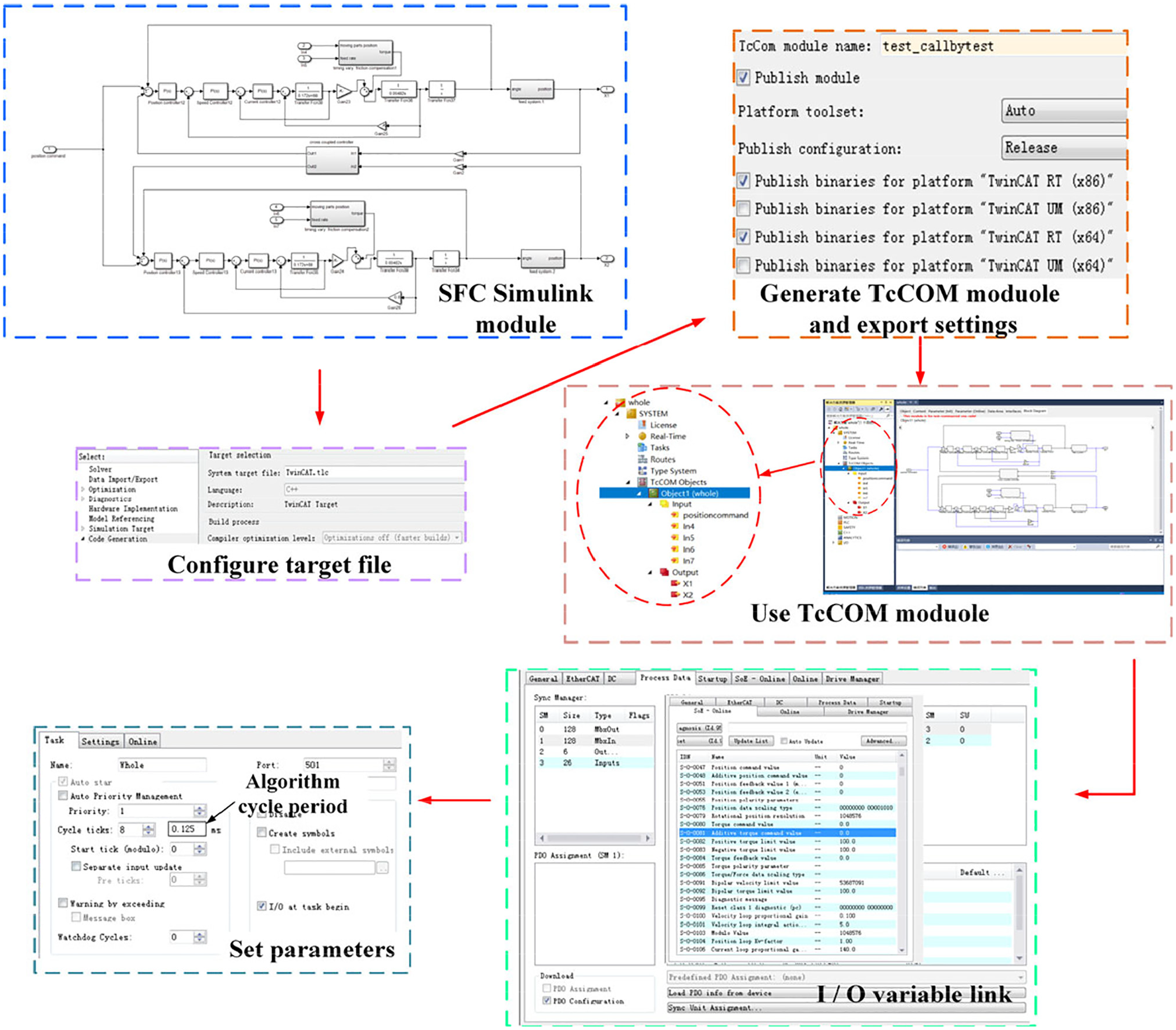
Process of SFC experiment.
CCSC (using P controllers) and Coulomb friction compensation (CFC) are compared with SFC to verify the effectiveness of this proposed method which can improve feeding accuracy. The CFC is a constant friction compensation method, and its friction compensation value is related to the mass of the crossbeam and moving parts (m1 and m2), but it cannot reflect the motion state of the DGMT. Based on IEC 61131-3 standard, writing programmable logic controller (PLC) program of CFC to compensate the friction force of the DDFMs. The tracking errors and non-synchronization errors are measured by two linear optical scales with a resolution of 0.1 μm. Set the positions of the moving parts l = 0, l = 0.3 m, and l = 0.6 m, the crossbeam moves at different feed rates such as v = 5 mm/s, v = 25 mm/s, and v = 50 mm/s. Each movement time is 10 s and the number of sampling points is 4000. The changes in tracking errors and non-synchronization errors during start-up, reverse, and stable operation are all monitored.
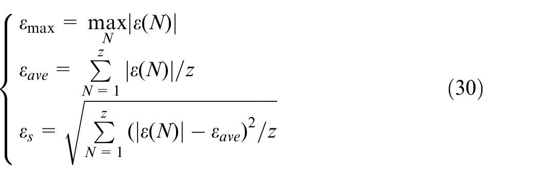
The position command curves under different feed rates are shown in Figure 16. The maximum error, average error, and error standard deviation are used as evaluation criteria to assess the performance of the proposed compensation method in terms of the single-axis tracking accuracy and the dual-axis synchronization accuracy, 35 and their expressions are shown in equations (29) and (30).
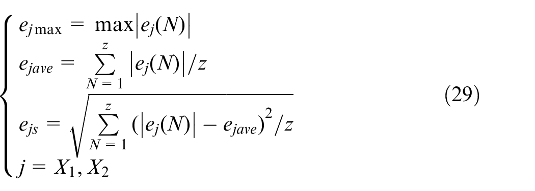
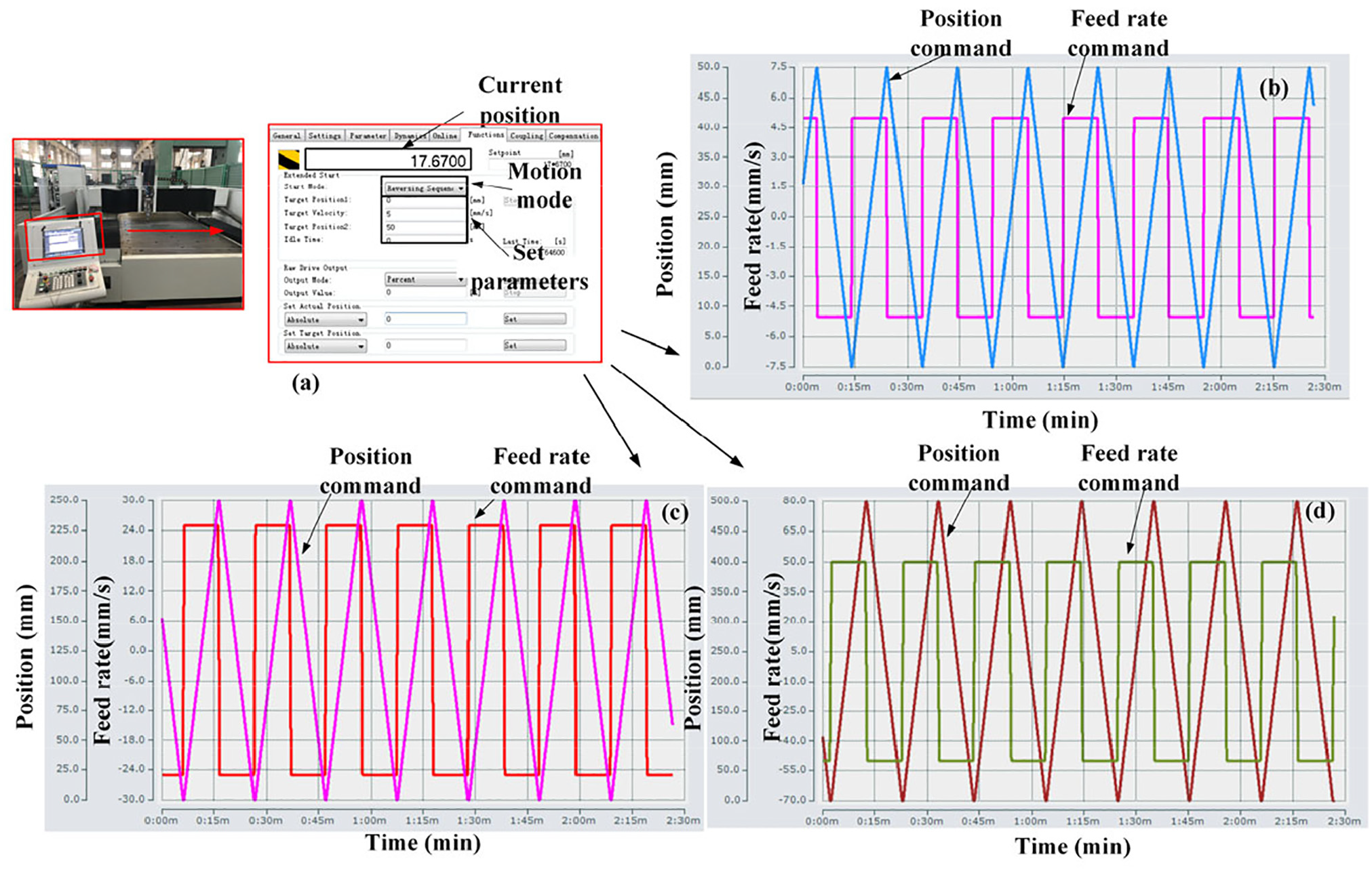
Experimental reference trajectory: (a) operating parameters setting, (b) the parameter of feed rate v = 5 mm/s, (c) the parameter of feed rate v = 25 mm/s, and (d) the parameter of feed rate v = 50 mm/s.
where
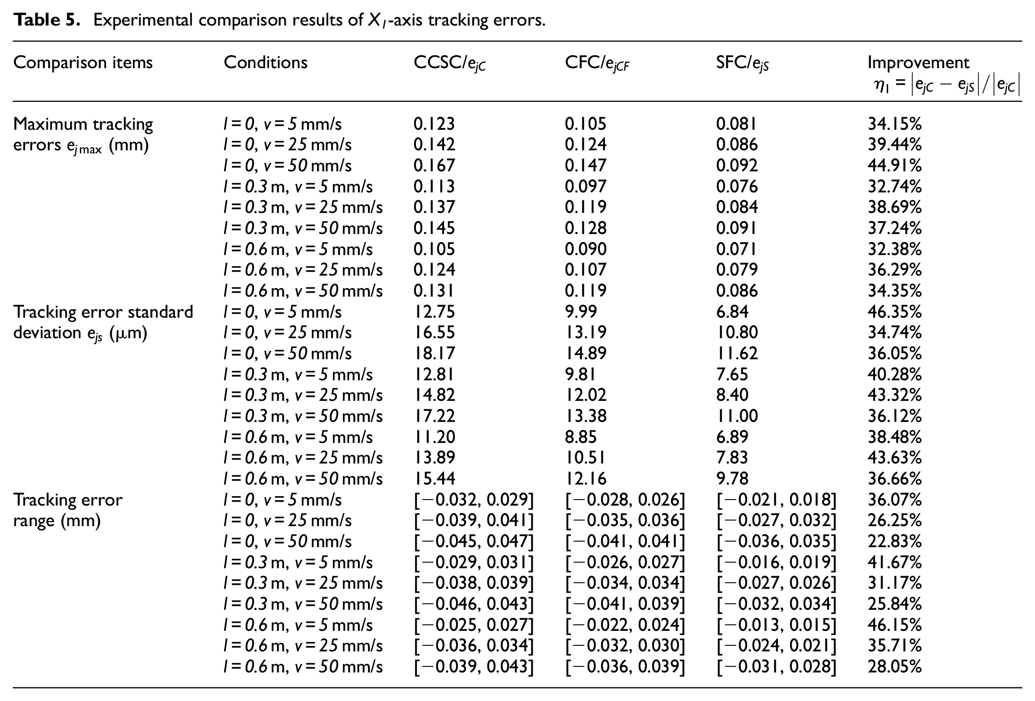
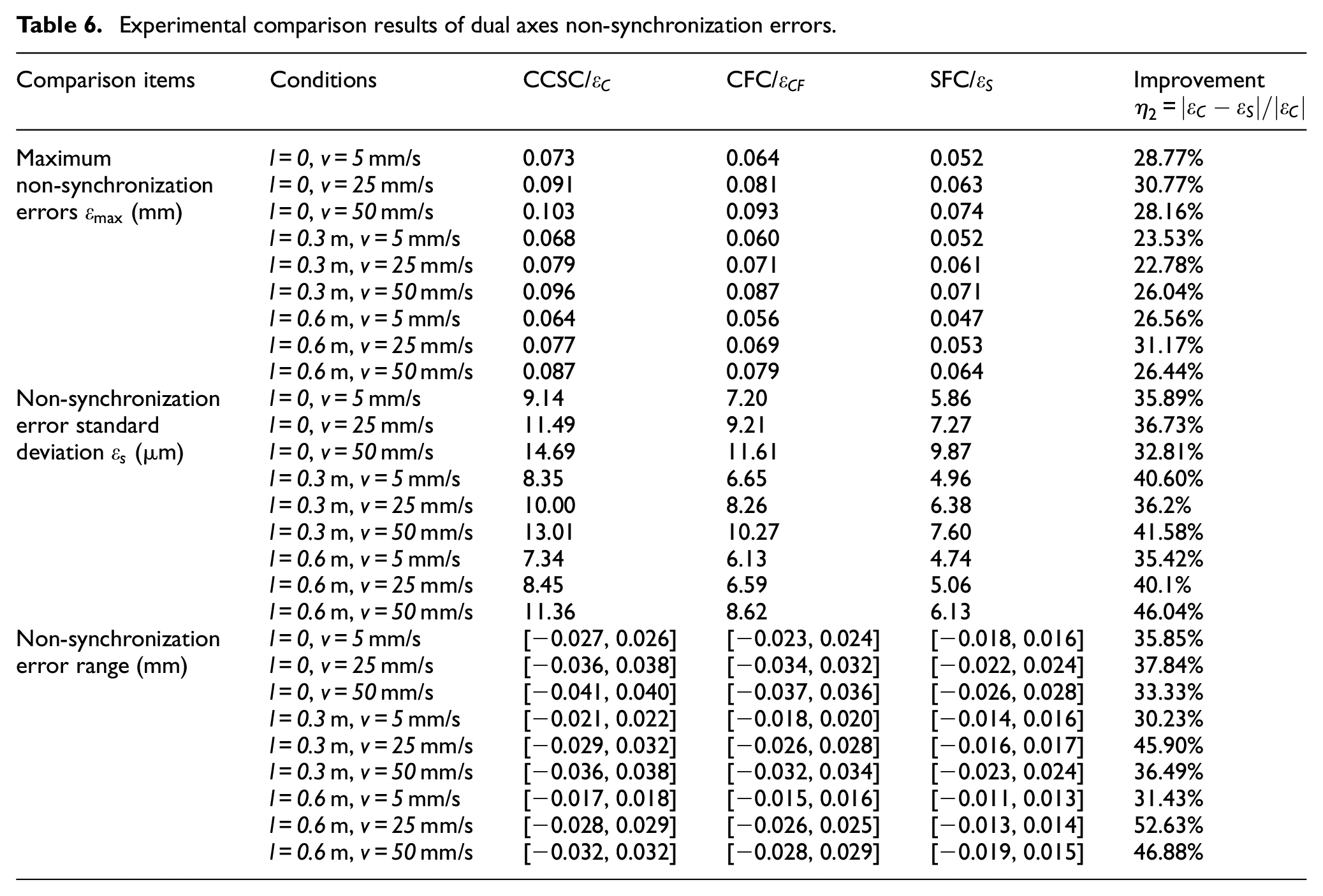
Figure 17 gives a typical experimental result among all the results. It can be seen that when the DGMT starts and reverses, the peak values of the tracking errors and the non-synchronization errors of CCSC are 0.123 and 0.073 mm, respectively. The ranges of the tracking errors and the non-synchronization errors are [−0.032, 0.029 mm] and [−0.027, 0.026 mm], respectively, when the system is in constant-speed operations. In the CFC, the ranges of the tracking errors and the non-synchronization errors are [−0.028, 0.026 mm] and [−0.023, 0.024 mm], respectively. The peak values of the tracking error and the non-synchronization error are 0.105 and 0.064 mm, respectively. When the SFC is adopted, and the ranges of the tracking errors and the non-synchronization errors are [−0.021, 0.018 mm] and [−0.018, 0.016 mm], respectively, when the system is in constant-speed operations. Furthermore, peak values of the tracking error and the non-synchronization error are effectively reduced, their value are 0.081 and 0.052 mm, respectively, in the events of starting and reversing. In the same way, the experimental comparison of the CCSC, CFC, and SFC under other conditions can be obtained. The above experimental results are summarized in Tables 5 and 6.
Experimental comparison results of X1-axis tracking errors.
Experimental comparison results of dual axes non-synchronization errors.
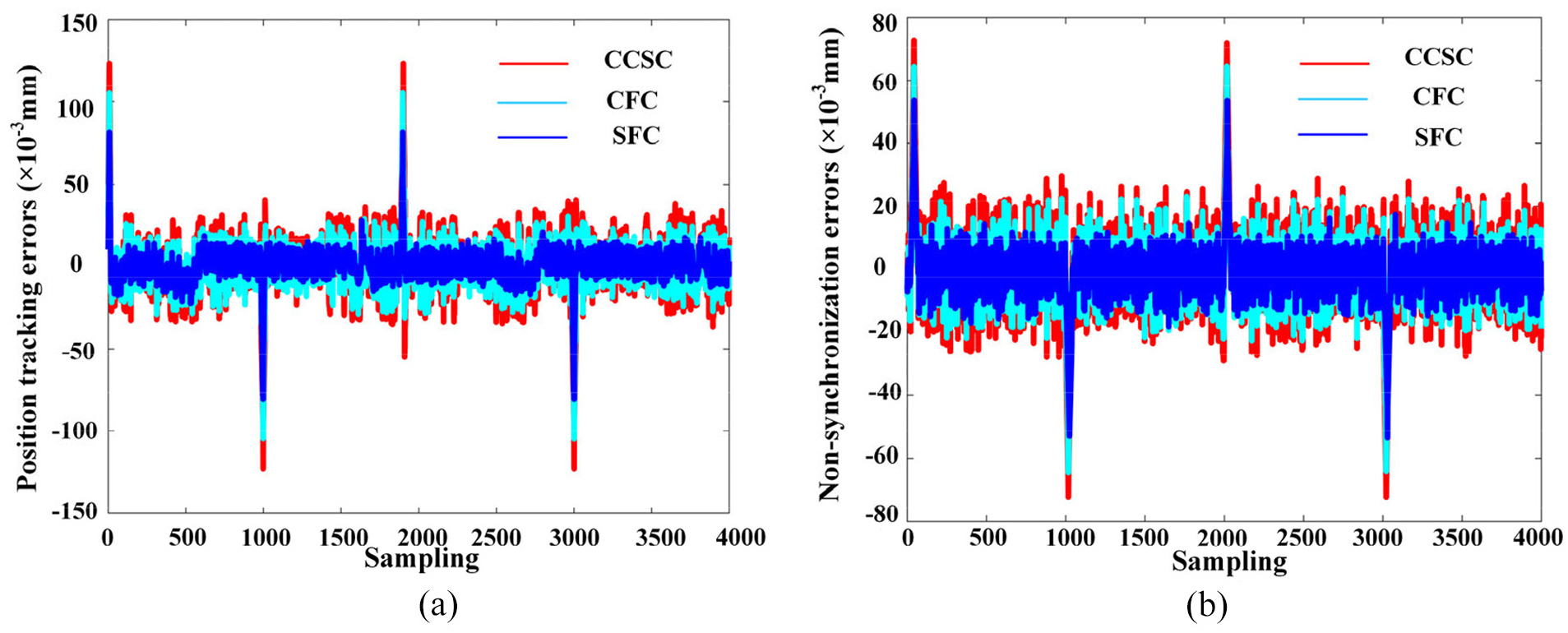
Comparison of experimental results CFC, CCSC, and SFC. Condition: l = 0 and v = 5 mm/s, the DGMT moves back and forth in the range of 0–50 mm: (a) tracking error comparison and (b) non-synchronization error comparison.
When the SFC is adopted, the peak values of the tracking errors and the non-synchronization errors during startup and reverse can be significantly reduced by 44.91% (167–92 μm) and 31.17% (77–53 μm), respectively. The tracking errors and non-synchronization errors during constant-speed operations can also be greatly reduced by 41.67% and 52.63%, respectively. Also, the maximum standard deviation of the tracking errors and the standard deviation of the non-synchronization errors can be reduced by 46.35% (12.75–6.84 μm) and 46.04% (11.36–6.13 μm), respectively. Tracking error standard deviation and non-synchronization error standard deviation are decreased effectively, which means the DGMT running stable in the motion process. In addition, due to the constant friction compensation, CFC is limited to reduce the tracking error and non-synchronization error of the DDFMs in the events of starting, reversing and constant-speed operations. This result complies with the simulation results and indicates that the proposed SFC can effectively improve the synchronization performance of the DDFMs.
Conclusions
The paper theoretically analyzes the position accuracy problem in the DDFMs, and establishes the SFC method. Experiments based on DGMT are carried out to compare the performance of the CCSC method, CFC method, and the proposed new compensation method (SFC). The experiment and simulation results verify that the SFC method can significantly improve the positioning accuracy of the DDFMs. The main conclusions are as follows:
This research builds a dynamic model that can reflect variations in the key joints’ stiffness of the DDFMs and friction forces’ effect on the feed drive system. Understanding this mechanical characteristic coupling is the basis of designing the error compensation method of dual feed drive systems. Through parameter identification experiments, a state-dependent friction model considering the influence of timing-vary factors (feed rates and dual-drive structure) on friction of dual axes is obtained. The motion performance of DDFMs can be further improved by considering the dynamic properties of friction and combination cross-coupled control strategy.
The experimental results show that compared with the CCSC and CFC, the SFC can reduce the standard deviation of tracking errors and non-synchronization errors by up to 46.35% and 46.04%, respectively. The range of position tracking and non-synchronization errors, as well as steady-state position errors can also be reduced. The proposed error compensation method can effectively improve feeding performance and stability of DDFMs, and it can be applied in a general dual-drive structure. Different from the compensation of a single feed drive system, the compensation of the DDFMs must consider the characteristics of double axes dynamic coupling. What is more, it also provides theoretical support for contour control of dual-drive machine tools.
Footnotes
Author contributions
Qi Liu: conceptualization, writing – original draft preparation, writing – review and editing, experiments; Hong Lu: conceptualization; Xinbao Zhang: methodology; Yongquan Zhang: validation and data; Yongjing Wang: writing – review and editing; Zhangjie Li: experiments; Meng Duan: experiments.
Declaration of conflicting interests
The author(s) declared no potential conflicts of interest with respect to the research, authorship, and/or publication of this article.
Funding
The author(s) disclosed receipt of the following financial support for the research, authorship, and/or publication of this article: This work was supported by the National Nature Science Foundation of China (no. 51675393) and the Hubei Province Intellectual Property “Three Major Projects”: Development of new straightening process and numerical control straightening technology for the motor shaft (Grant no. 2019-1-76).