Sage Journals: Discover world-class research

Abstract

The main purpose of this paper is to demonstrate the applicability of conventional cutting tools in the machining of a custom tibial insert of a knee prosthesis. This study also aims to reduce the roughness and minimise the production time. In this work, the optimisation of cutting strategies and parameters was achieved through the design and construction of a test-part containing the most important complex surfaces of the femoral cavities, the focus of the study. The milling was carried out in accordance with the Design Of Experiment and the Taguchi method and was performed in two stages to reduce the number of analysed factors. The achieved parameters are applied to the machining of a modelled tibial insert made of UHMWPE, using a NC machine with three axes. The initial parameters studied were the cutting method, axial and radial depth of cut, the direction of the feed and the feed rate. Three strategies were studied: two Blend, resulting in radial and spiral toolpaths, and one Parallel. According to the spiral strategy, an arithmetical mean roughness of R_a = 1.1 µm was obtained, representing an improvement of 45% relatively to the initial phase value of 2.0 µm, with the Parallel toolpath. An overall improvement of 34% in time efficiency of the finishing operation was achieved after changing the machine settings. This study supports the conclusion that high-speed milling is an expeditious process to produce customised tibial inserts.

Keywords

Knee prosthesis tibial insert high speed machining UHMWPE optimisation milling toolpaths cutting parameters

Introduction

Total knee arthroplasty (TKA) is an intervention, developed in the 1970s, consisting of replacing the joint between the femur and tibia and between the femur and patella.¹ In OECD countries, more than 1.6 million knee replacement surgeries are performed annually, and between 2000 and 2015 the rate of these surgeries increased almost 100%.² It is estimated that part of these surgeries, between 7% and 10%, are revision procedures.³ The failure of the primary surgeries is due to factors such as, the durability of the prosthesis and the degree of precision verified in its placement. Furthermore, TKA is also performed on increasingly younger patients, which demands a more lasting result.⁴ A recent review concluded that approximately 82% of total knee replacements have a lifetime of 25 years,⁵ which is not enough for younger patients. The economic impact due to these factors can only be mitigated, achieving greater efficiency in primary surgeries, reducing the need for revision procedures and simultaneously increasing the durability of the prosthesis components.

The time spent on surgery can be reduced with the use of customised cutting jigs, obtained with rapid prototyping techniques, and a better implant alignment is achieved with the spreading of new techniques, like computer-assisted TKA.⁶ Together, these techniques increase implant survivorship and can also be associated with customised prostheses, allowing the use of dimensions or shapes that are more suitable to the patient’s bone, without the constraints of using the available standard dimensions.⁷ These approaches use data from preoperative imaging studies, such as magnetic resonance imaging or computerised tomography as a starting point,^8,9 generating the 3D design of the patient’s bone. This model is used both in the preparation and virtualisation of the surgery, as well as in the implant’s customisation. However, it is still necessary to convert the mass production process to the manufacture of customised prostheses. Even the recent application of the additive technology in the manufacture of customised UHMWPE tibial inserts by selective laser sintering¹⁰ requires additional machining operations in the femoral cavities to achieve the necessary surface quality. This paper shows and demonstrates the applicability of high speed machining in the unitary production of knee prosthesis components.

TKA prosthesis, shown in Figure 1(a), consists of a femoral component, a tibial tray, an interface between these two components, know as a tibial insert, and a patellar component, if needed.

Figure 1.

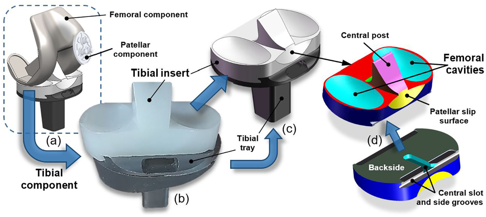
(a) Knee prosthesis, tibial component of a: (b) real and (c) CAD model, and (d) tibial insert (top and back side views).

The UHMWPE, due to its properties,^11–13 is the material used since the late 1960s and is still today the “golden standard” polymer used in the manufacture of the patellar component and tibial insert,¹⁴ whether in fixed or mobile bearing designs.^15,16

There are many different designs of prostheses on the market¹⁷ and they essentially follow two main approaches that emerged in the 1970s and are still used today: anatomical and functional.¹⁸ In the anatomical approach, the design allows the preservation of all or most of the soft tissues of the natural knee (anterior and posterior cruciate ligaments). In the functional designs, the non-anatomic surfaces are used to maximise the contact area, decreasing the stress forces in the polyethylene insert. Given the variety of existing configurations, this article focuses on the manufacturing process of a posterior-stabilised (PS) fixed bearing insert, that follows a functional approach, as can be seen in Figure 1. This type of design incorporate a central post in the polyethylene component that fits into the femoral component, preventing displacement in the medial-lateral direction and reducing the risk of femur-tibial dislocation. Figure 1(c) and (d) show a CAD drawing of the insert made from a real model, pointing out the most important surfaces in contact with other components. This tibial insert is the prototype machined as an application of both strategy and cutting parameters optimisation.

The femoral cavities, identified in Figure 1(d), allow the sliding movement of the femoral component, being subjected, in certain areas, to high stresses occurring at a reduced or near zero speed.¹⁹ These conditions make the lubrication by synovial fluid more difficult and cause higher local wear. The femoral cavities are the most sensitive surfaces of the tibial insert and they have a complex geometry.

Problems with wear and fatigue damage of the UHMWPE have always limited the longevity of the knee prosthesis.^5,20 One of the main causes of failure is the aseptic loosening of implants due to an adverse reaction of the body, called osteolysis. Smaller particles generated from wear can stimulate an osteolytic response and the manufacturing process of the tibial insert can influence the clinical duration of the prosthesis.^12,21

Many factors influence the wear mechanisms of UHMWPE tibial implants during in vivo friction, namely: machining process factors (metal counter face roughness, UHMWPE surface topography), implant design, surgical technique (knee alignment) and patient factors (body weight, synovial fluid properties).^21,22 On the machining process factors, it has been shown that the polyethylene surface morphology, obtained by high speed machining, leads to a low friction coefficient in laboratory tests and less degradation of the surface.²³ However, there is limited information on the effect of machining parameters on UHMWPE tribological properties.^{13,21,23–26} This paper focuses on machining process variables, and, more precisely, on the main outcome factor, roughness.

Roughness can be predicted according to several approaches based on experimental investigation,^27–32 machining theory³³ and numerical methods.^34,35 However, the latter is not yet wide spread in CAM software. The strategies and cutting parameters are typically information protected by the prosthesis manufacturers, and there is limited information available on the impact of these choices on roughness. The present study reports the impact of various machining scenarios on the surface finish of the femoral cavities of prosthesis. The approach followed in this article is based on experimental investigation.

Materials and methods

Different parameter combinations were studied using conventional cutting tools. The experiments were performed using a test-part and were planned according to the DOE method, based on Taguchi, in order to reduce the number of experiments performed. This method is commonly used in the optimisation of machining parameters.^36–43 The experimental plan was developed in two stages. The final goal is to determine the best strategy and parameters to minimise the arithmetical mean roughness value (R_a). In both stages, three levels of each factor are used, allowing probing non-linear behaviour. Main effects plots, response tables and variance analyses (ANOVA) statistical comparisons were used to evaluate the results. The outcome from the predicted optimised parameters was verified by an independent test.

First stage of testing

In this first stage, the factors that most influence the surface quality of the toroidal cavities were identified. The cutting parameters controlled during the experiments were spindle speed (n), feed rate (f_z), effective cutting speeds, and axial (a_p) and radial (a_e) depth of cut. In addition to these variables, toolpath and machining strategies, which include the direction of the feed, were also tested. These parameters are defined in Figure 2, emphasising the differences between two methods of cutting, up-milling (the feed direction of the cutting tool is opposite to its rotation) and down-milling (the cutting tool is fed in the direction of rotation).

Figure 2.

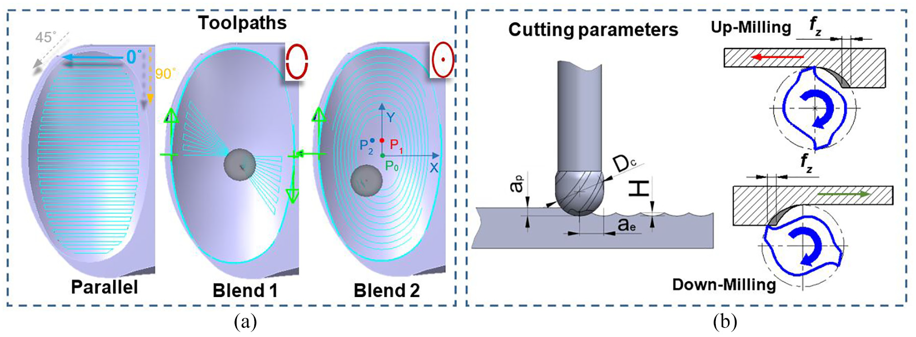
Toolpaths used to finish the insert cavities: (a) Parallel and Blend with reference lines marked in red in the upper right corner, given as across and along, respectively and (b) definition of the cutting parameters.

Four main factors were selected for each toolpath and, after analysis of the results, were ordered by their influence on the R_a response variable. Through previous simulations in Mastercam X6, three toolpaths were selected to perform the finishing of the cavities: Parallel and two Blend variants, Figure 2.

In Blend 1 strategy, the reference lines (chains), picked in the Mastercam as across, were the contour of the cavity divided into two, creating a trajectory similar to the radial one, but running through the cavity from one end to the other. In Blend 2 strategy, the contour and a point were indicated as along, resulting in a spiral or, optionally, an elliptical trajectory.

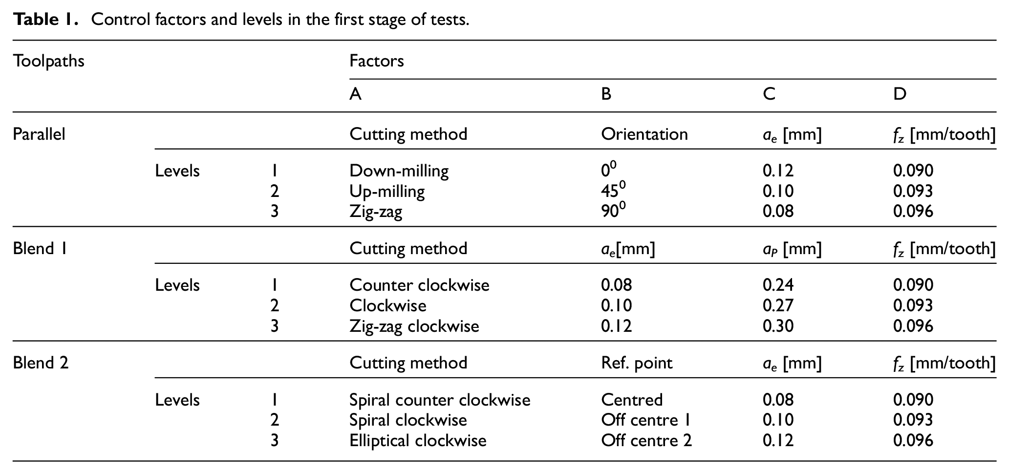
The three strategies generated three groups of distinct trials due to the specificity of the factors used in each one. Four factors were selected in each toolpath. The common parameters were the cutting method, f_z and a_e, shown in Figure 2. For the Parallel strategy, the fourth factor was the orientation of the toolpath, with zero degrees corresponding to the direction along the minor axis of the elliptical contour, 90° along the major axis and, finally, 45° relative to the previous axes, Figure 2. In the Blend 1 toolpath (radial type), the axial depth of cut was added which is coincident with the value of the over-thickness left by the semi-finishing operation. For the Blend 2 strategy, the location of the reference point also varied: in the centre of the cavity (P₀), in position 1 (P₁; X₁ = 0 mm, Y₁ = 6 mm) and position 2 (P₂; X₂ = −4 mm, Y₂ = 6 mm), Figure 2. The factors and their respective levels are summarised in Table 1. In the toolpaths tested, the maximum distance between passages was 0.12 mm. In accordance with the theoretical equations of crest height and arithmetic mean deviation of the profile defined by Quintana,³³ a profile height of H = 0.60 μm andR_{a theoretic} = 0.30 µm, were determined, consideringa ø= 6 mm ball end mill and a_e = 0.12 mm in a flat plane. However, the femoral surface is not flat. Furthermore, the cutting of material is an intermittent action, that is, in the feed direction, the roughness is also affected by the selected value of the feed rate. For flat surfaces where f_z = 0.096 mm/tooth, the maximum crest of height will be H = 0.38 μm.³³ For the Parallel strategy, the down-milling and up-milling levels characterise the cutting method in the first half of the cavity, because in the second half, the material appears on the opposite side. The experiment plan was drawn up using orthogonal array L₉ (3⁴) – four factors with three levels each.

Table 1.

Control factors and levels in the first stage of tests.

Toolpaths			Factors
			A	B	C	D
Parallel			Cutting method	Orientation	a_e [mm]	f_z [mm/tooth]
	Levels	1	Down-milling	0⁰	0.12	0.090
		2	Up-milling	45⁰	0.10	0.093
		3	Zig-zag	90⁰	0.08	0.096
Blend 1			Cutting method	a_e[mm]	a_P [mm]	f_z [mm/tooth]
	Levels	1	Counter clockwise	0.08	0.24	0.090
		2	Clockwise	0.10	0.27	0.093
		3	Zig-zag clockwise	0.12	0.30	0.096
Blend 2			Cutting method	Ref. point	a_e [mm]	f_z [mm/tooth]
	Levels	1	Spiral counter clockwise	Centred	0.08	0.090
		2	Spiral clockwise	Off centre 1	0.10	0.093
		3	Elliptical clockwise	Off centre 2	0.12	0.096

Second stage of tests

In the second test stage, the two most relevant factors resulting from the ordering of stage 1 were selected for further analysis; for the remaining factors, the optimal level determined in stage one was used. The factors continued with three levels. The maximum resolution of the L₉ (3²) array (factorial) was used to define the experiments. The reduced matrices of Taguchi used in the first stage of tests, the complete factorial arrangements of the second phase, and the statistical treatment of the results were performed through Minitab 17 software.

Confirmation experiments

The last step in the Taguchi method is to carry out new tests that confirm the results from the optimal levels of each factor, obtained in previous experiments. In addition, the most important factor was tested in six levels, keeping the remaining factors at their optimal level, in order to make the adjustment line more significant. Thus, the regression equation was adjusted considering six values: the three points from the levels tested in the second stage, the two intermediate points and a last point outside the previously tested domain. The selected side of this last point was the one that optimised the R_a parameter. The points considered are all equidistant and each experiment was replicated twice.

Test-part definition

In the design of a test-part, the main geometric forms of the prosthesis are summarised and reproduced. This concept, commonly used in the optimisation of machining parameters, facilitates the execution of the experiments and allows a direct comparison of the results.^41,44–47 After the optimisation of the parameters in the test-part, these are applied in the manufacture of the final component. The need to use nine tests for each toolpath led to the design of a test-part with nine cavities in a polyethylene block with approximate dimensions of 177 × 103 × 20 [mm]. Based on the analysis of real tibial inserts, the femoral cavities were simplified and parameterised as part of the surface of a doughnut, Figure 3. The radius of revolution of the cross-section measures 37 mm. The transverse circular section has a radius of 23 mm, resulting in a cavity with a 60 mm longitudinal outer radius. The cavity has a maximum depth (at the central point) equal to 5 mm, a maximum width of 48 mm and a minimum of 29 mm, approximately. The test-part also incorporates other geometric elements, such as contours with various radii of curvature, spherical slices and slots. A test-part in each replication was machined and each experiment was replicated twice.

Figure 3.

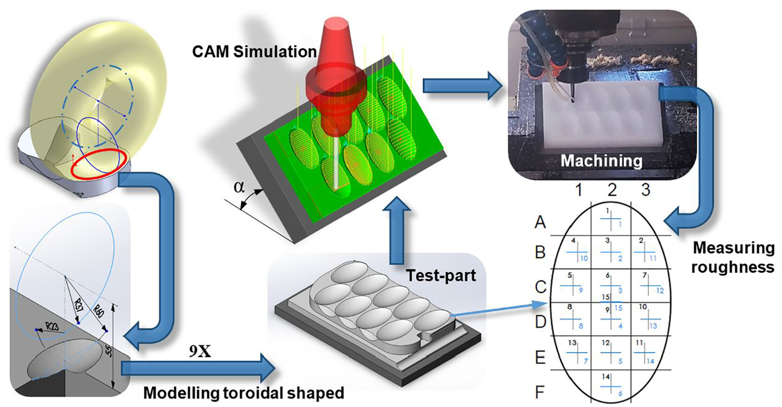
CAD modelling, CAM simulation, machining and measuring the test-part used in the experiments.

Simulation and machining

The trajectories were generated and simulated using Mastercam X6 software and the post-processed programs were introduced in the CNC machine with tree axes, Figure 3. In the first stage of tests, the axis of rotation of the end mill was perpendicular to the upper surface of the initial stock, α = 0° illustrated in Figure 3. In the remaining tests, the initial stock was tilted 45° relative to the same axis (α = 45°). The roughing of the cavities was performed with the same strategy, parameters and cutting tool. The semi-finishing operation was performed with the same cutter, using the area clearance strategy, producing a spiral toolpath and leaving a uniform over thickness equal to the axial depth of cut with the Blend 1 trajectory and 0.3 mm in the other cases. In the finishing operations a 6 mm ball solid carbide end mill was used, with two teeth and a flute helix angle of 50°, and a spindle speed of n = 9500 rpm. The cooling of the workpiece and tool was performed with compressed air, directed at the cutting interface.

Evaluation of the surface quality of the cavity

The experimental assembly used to obtain the surface roughness readings in the cavities consists of a manual column stand with a platform that supports the test-part, on a levelling table, where the drive unit was supported, and on a display unit control that stores data. The surface finish was measured in 15 zones per cavity. In each zone, two readings were taken along perpendicular directions. Thus, each cavity was evaluated by the average of 30 readings with positions as shown in Figure 3. The R_a value that characterises each experiment was calculated by the mean of the two replicates of the cavity. The contact roughness tester had a standard stylus, with 0.75 mN of measuring force and 2 μm tip radius. The reading conditions considered a R profile with digital Gaussian filter, 800 μm of measuring range (0.01 μm resolution), 0.5 mm/s of reading speed, 0.8 mm of cut-off length, and a total evaluation length of 4.0 mm (number of sampling lengths = 5), making the total travel length of the detector 4.8 mm.

Results and discussion

First stage of testing

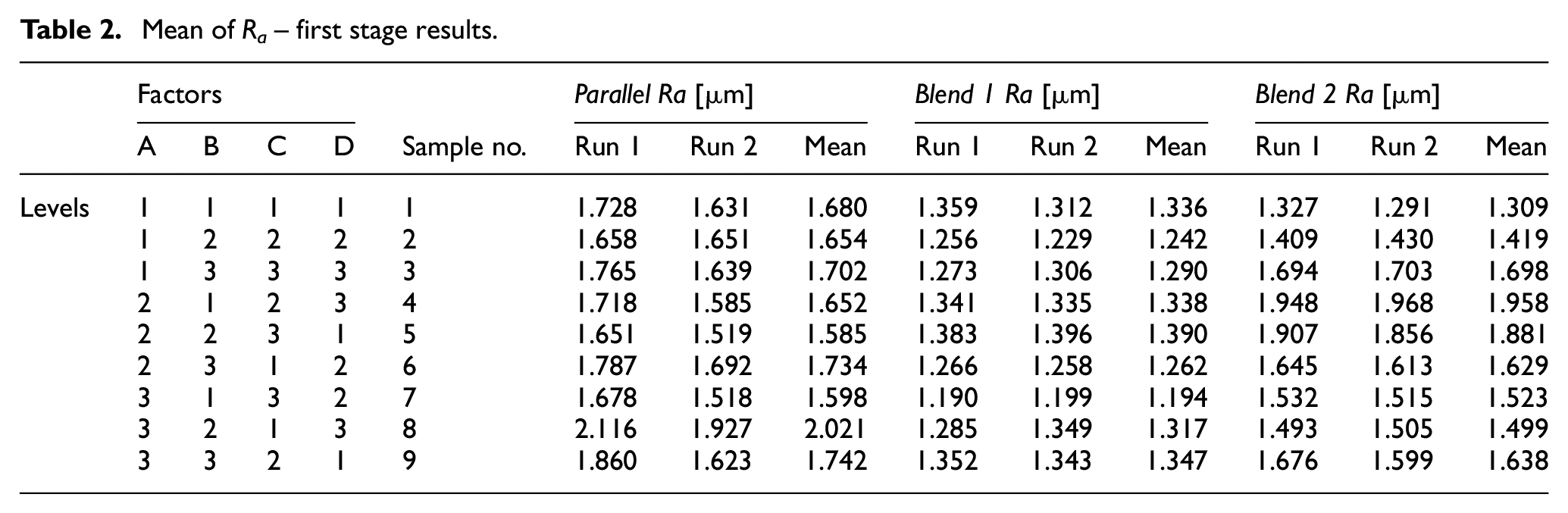
The combination of the levels and the results obtained for each test, as well as their mean, are shown in Table 2. The optimal levels of each factor and the response tables for the R_a parameter of the three toolpath tested were determined based on these results. The optimal levels were A2-B1-C3-D2, with the Parallel toolpath, A3-B1-C3-D2, with Blend 1 strategy and A1-B1-C1-D2, with the Blend 2, minimising the value of the R_a parameter. In all trajectories, the optimum level for the feed rate was the intermediate level of f_z = 0.093 mm/tooth, and for the a_e was the lowest value of 0.08 mm. The lower mean R_a = 1.19 µm was obtained in sample 7 of the Blend 1 strategy, where all the optimal levels of each factor were used. This strategy also presented the smaller variation in the nine cavities, essentially due to the lower results observed in the centre of the surface, where the cutter passed several times. Analysing the value of R_a by zone, the centre of the cavity had poor finishing on all the toolpaths, especially on the Parallel with R_a = 3.38 µm (the mean of all experiments in the middle region: cells C2, D2 and centre, Figure 3). The central zone, visibly affected by this effect, has a length of approximately 18 mm, which means that the central part of the ball end mill, with a radius of less than 0.45 mm, produces a very low effective cutting speed, whose minimum value is zero at the central point. To prevent contact between the milling cutter and the cavity surface from distances of less than 0.45 mm, the test-part must be tilted at least α = 32.2°, so that the cutter does not machine in a level below the affected area. With the Blend 2 toolpath, changing the location of the middle point did not avoid a worse finishing of the central zone. The centred trajectory minimises the operating time by shortening the total distance travelled by the tool, used in the following experiments.

Table 2.

Mean of R_a– first stage results.

	Factors					Parallel Ra [µm]			Blend 1 Ra [µm]			Blend 2 Ra [µm]
	A	B	C	D	Sample no.	Run 1	Run 2	Mean	Run 1	Run 2	Mean	Run 1	Run 2	Mean
Levels	1	1	1	1	1	1.728	1.631	1.680	1.359	1.312	1.336	1.327	1.291	1.309
	1	2	2	2	2	1.658	1.651	1.654	1.256	1.229	1.242	1.409	1.430	1.419
	1	3	3	3	3	1.765	1.639	1.702	1.273	1.306	1.290	1.694	1.703	1.698
	2	1	2	3	4	1.718	1.585	1.652	1.341	1.335	1.338	1.948	1.968	1.958
	2	2	3	1	5	1.651	1.519	1.585	1.383	1.396	1.390	1.907	1.856	1.881
	2	3	1	2	6	1.787	1.692	1.734	1.266	1.258	1.262	1.645	1.613	1.629
	3	1	3	2	7	1.678	1.518	1.598	1.190	1.199	1.194	1.532	1.515	1.523
	3	2	1	3	8	2.116	1.927	2.021	1.285	1.349	1.317	1.493	1.505	1.499
	3	3	2	1	9	1.860	1.623	1.742	1.352	1.343	1.347	1.676	1.599	1.638

With Parallel toolpath, the up-milling or down-milling method produced very similar results. This is justified due to the switching of the cutting method from up-milling in the first half of the cavity to down-milling in the second half and vice versa. As expected, the overall result of these two levels is identical and achieves a better finish compared to that in which the material is removed in both forward and backward paths (zig-zag level). The best orientation for this toolpath was zero degrees, along the minor axes of the cavity contour.

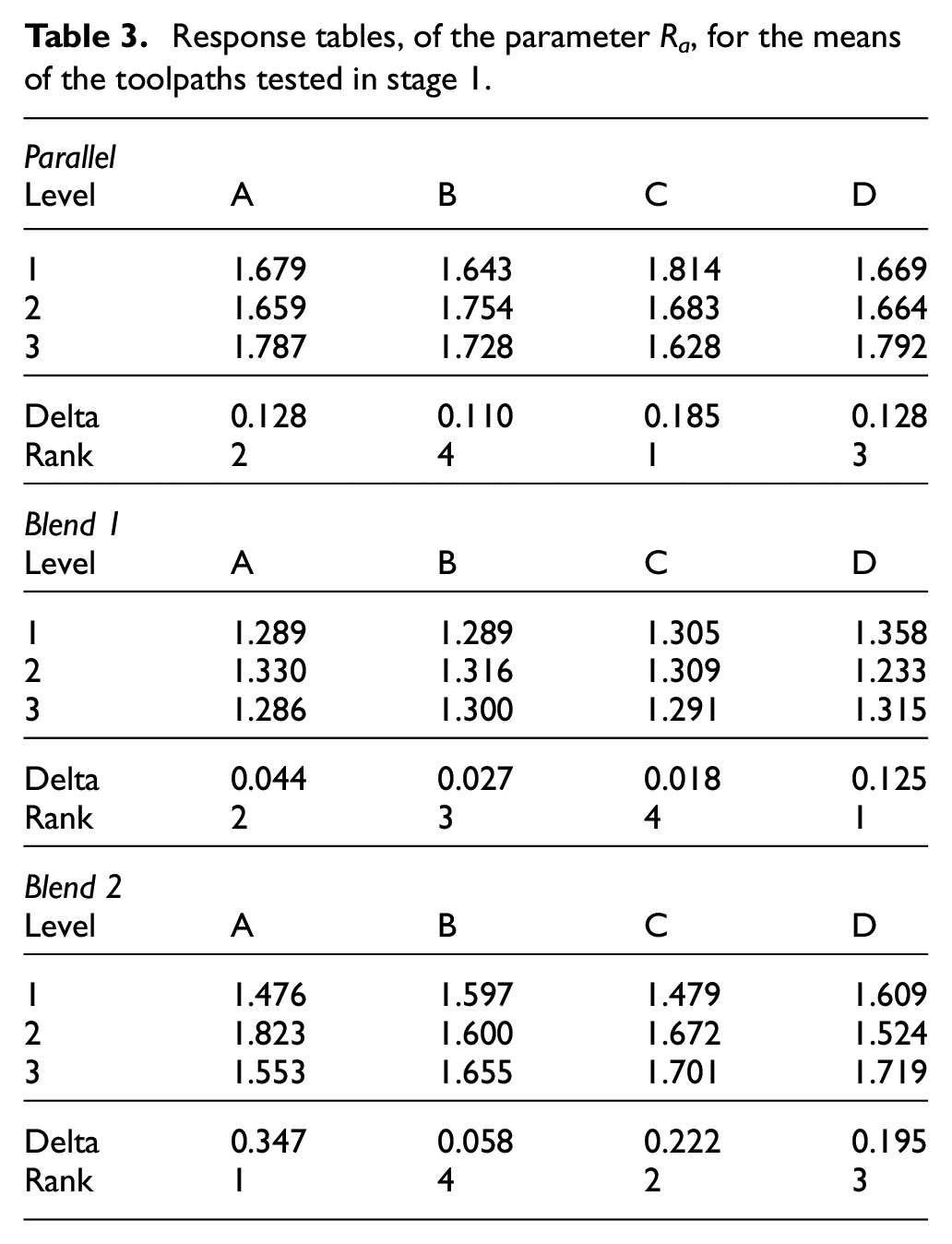
The response tables allowed the ranking of each fact or on the R_a parameter for the three toolpaths, in Table 3. In the two most important parameters, the cutting method was included in all toolpaths. The a_e was the first and second most important factor for the Parallel and Blend 2 respectively, while for Blend 1, the most significant parameter was the feed rate. With Blend 1, the a_p and a_e caused small variations in roughness. The Blend 2 toolpath is the one with the greatest variation between levels, with a greater capacity to be optimised in the second testing stage.

Table 3.

Response tables, of the parameter R_a, for the means of the toolpaths tested in stage 1.

Parallel
Level	A	B	C	D
1	1.679	1.643	1.814	1.669
2	1.659	1.754	1.683	1.664
3	1.787	1.728	1.628	1.792
Delta	0.128	0.110	0.185	0.128
Rank	2	4	1	3
Blend 1
Level	A	B	C	D
1	1.289	1.289	1.305	1.358
2	1.330	1.316	1.309	1.233
3	1.286	1.300	1.291	1.315
Delta	0.044	0.027	0.018	0.125
Rank	2	3	4	1
Blend 2
Level	A	B	C	D
1	1.476	1.597	1.479	1.609
2	1.823	1.600	1.672	1.524
3	1.553	1.655	1.701	1.719
Delta	0.347	0.058	0.222	0.195
Rank	1	4	2	3

Second stage of testing

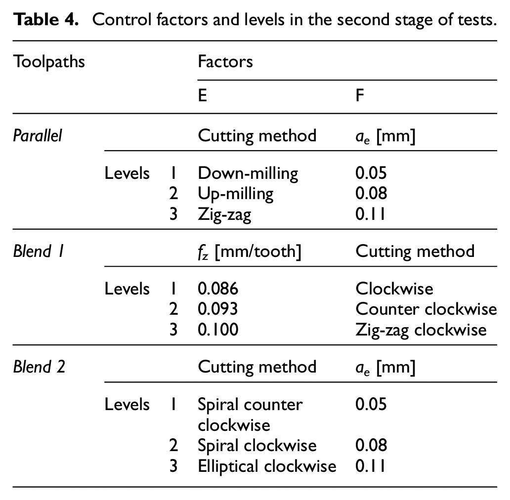
The levels were adjusted seeking to obtain lower values of roughness. The optimum level of the previous tests was selected as the intermediate level of this stage. The extreme values have been adjusted so that their mean was the new intermediate level and differences between levels were also increased. The factors and their new levels are presented in Table 4. The machining tests of this stage used the new slope of the cavities (α = 45°) in the three strategies. According to this change, the Parallel strategy now has three full levels in the cutting method, allowing the same cutting method across the surface.

Table 4.

Control factors and levels in the second stage of tests.

Toolpaths			Factors
			E	F
Parallel			Cutting method	a_e [mm]
	Levels	1	Down-milling	0.05
		2	Up-milling	0.08
		3	Zig-zag	0.11
Blend 1			f_z [mm/tooth]	Cutting method
	Levels	1	0.086	Clockwise
		2	0.093	Counter clockwise
		3	0.100	Zig-zag clockwise
Blend 2			Cutting method	a_e [mm]
	Levels	1	Spiral counterclockwise	0.05
		2	Spiral clockwise	0.08
		3	Elliptical clockwise	0.11

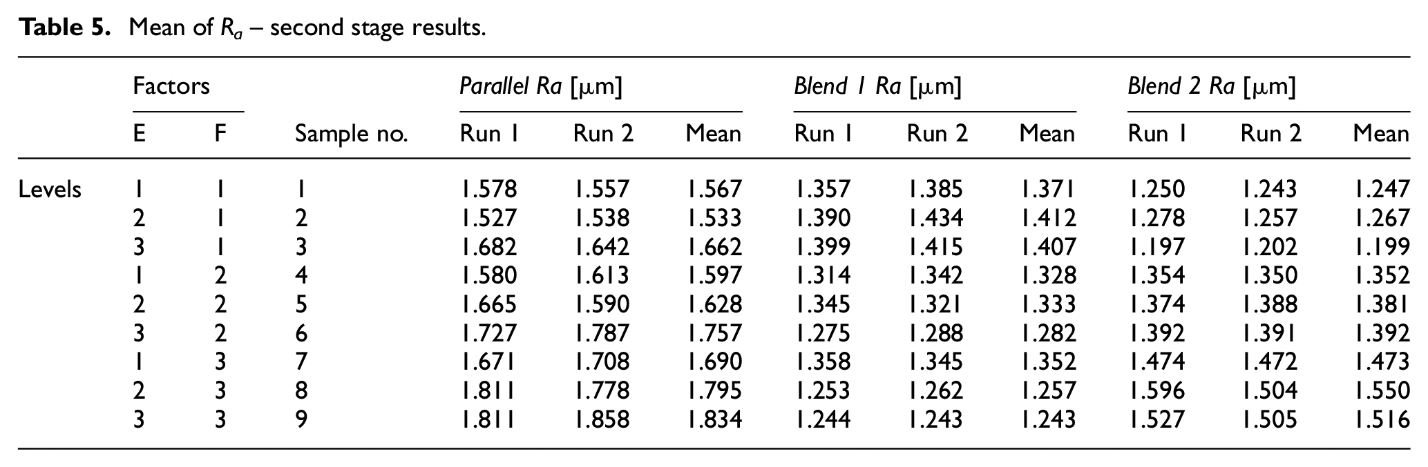
The new combination of the levels and the results of R_a in each test are provided in Table 5. Their analysis shows that sample 3 of the Blend 2 strategy reached the lowest mean, R_a = 1.20 µm, using the smallest increment (a_e = 0.050 mm) and the elliptical cut method. The worst value, R_a = 1.83 µm, was obtained for sample 9 of the Parallel trajectory, which applied the higher increment (a_e = 0.11 mm) and the double-direction cut method. This last trajectory has, on average, R_a = 1.67 µm, the worst result. The wider range in results continued to belong to the Blend 2 strategy, showing a higher sensitivity to the tested factors.

Table 5.

Mean of R_a– second stage results.

	Factors			Parallel Ra [µm]			Blend 1 Ra [µm]			Blend 2 Ra [µm]
	E	F	Sample no.	Run 1	Run 2	Mean	Run 1	Run 2	Mean	Run 1	Run 2	Mean
Levels	1	1	1	1.578	1.557	1.567	1.357	1.385	1.371	1.250	1.243	1.247
	2	1	2	1.527	1.538	1.533	1.390	1.434	1.412	1.278	1.257	1.267
	3	1	3	1.682	1.642	1.662	1.399	1.415	1.407	1.197	1.202	1.199
	1	2	4	1.580	1.613	1.597	1.314	1.342	1.328	1.354	1.350	1.352
	2	2	5	1.665	1.590	1.628	1.345	1.321	1.333	1.374	1.388	1.381
	3	2	6	1.727	1.787	1.757	1.275	1.288	1.282	1.392	1.391	1.392
	1	3	7	1.671	1.708	1.690	1.358	1.345	1.352	1.474	1.472	1.473
	2	3	8	1.811	1.778	1.795	1.253	1.262	1.257	1.596	1.504	1.550
	3	3	9	1.811	1.858	1.834	1.244	1.243	1.243	1.527	1.505	1.516

The R_a values measured in the central zone of the cavity are lower than those measured in the first stage and more uniform relative to the other regions. This is justified by the absence of abrasion of the surface through the central part of the milling cutter. This improvement ensures that there is always a real cut across the cavity. The mean value of all the cavities in the central zone is 1.62 µm with the Parallel toolpath, 0.98 µm for the Blend 1 and 1.21 μm for the Blend 2 strategy, showing that tilting the workpiece 45° avoids the abrasion issue. The Blend 1 toolpath continues to benefit from the multiple passages in the central zone; however, the differences are now much smaller, compared to the other two trajectories.

With the Blend strategies, there are some zones with mean values of R_a lower than 1 μm, whose lowest value is 0.8 μm with Blend 2. The main effect graph in Figure 4 presents the optimal levels of each factor for the three toolpaths: E1–F1, for the Parallel strategy, E3–F3, for the Blend 1 strategy and E1–F1, for the Blend 2 strategy. The optimum level of a_e was registered for the lowest value 0.05 mm (Parallel and Blend 2). With the best trajectory, Blend 2, the most suitable cutting method was the spiral counter clockwise direction, but the differences between the three levels are very small, less than 0.042 µm, shown in Table 6. On the opposite side, the factor with the most impact (delta = 0.275 µm) is the a_e, with practically linear behaviour, Figure 4.

Figure 4.

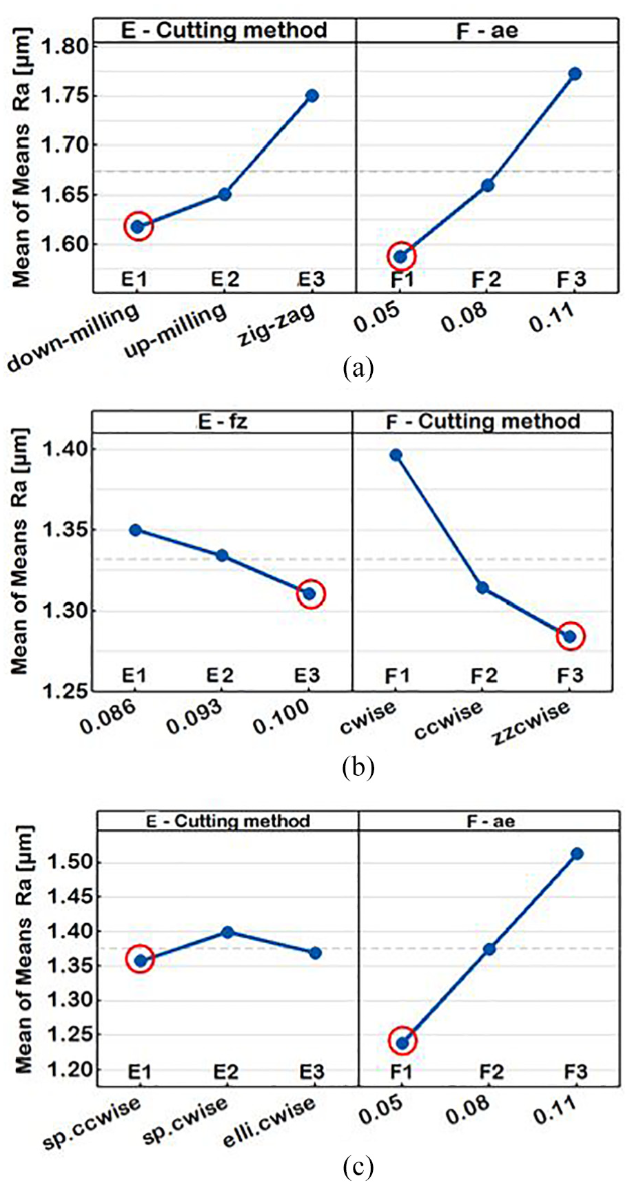
Main effects plots for R_a means to the toolpaths of stage 2: (a) Parallel, (b) Blend 1 and (c) Blend 2.

Table 6.

Response tables of the R_a parameter, for the means of the toolpath tested in stage 2.

Parallel			Blend 1			Blend 2
Level	E	F	Level	E	F	Level	E	F
1	1.618	1.587	1	1.350	1.397	1	1.369	1.238
2	1.652	1.660	2	1.334	1.314	2	1.357	1.375
3	1.751	1.773	3	1.311	1.284	3	1.399	1.513
Delta	0.133	0.186	Delta	0.039	0.113	Delta	0.042	0.275
Rank	2	1	Rank	2	1	Rank	2	1

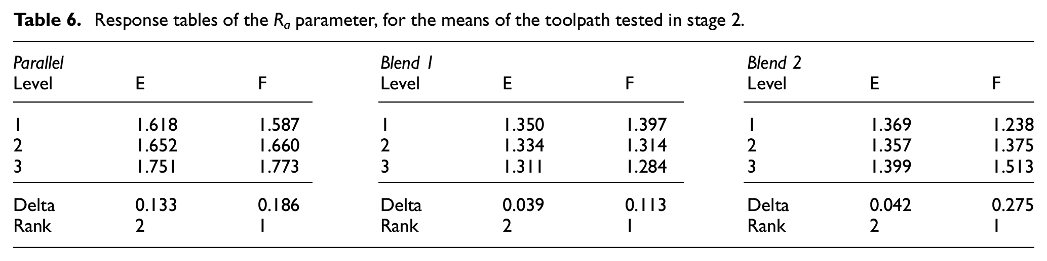
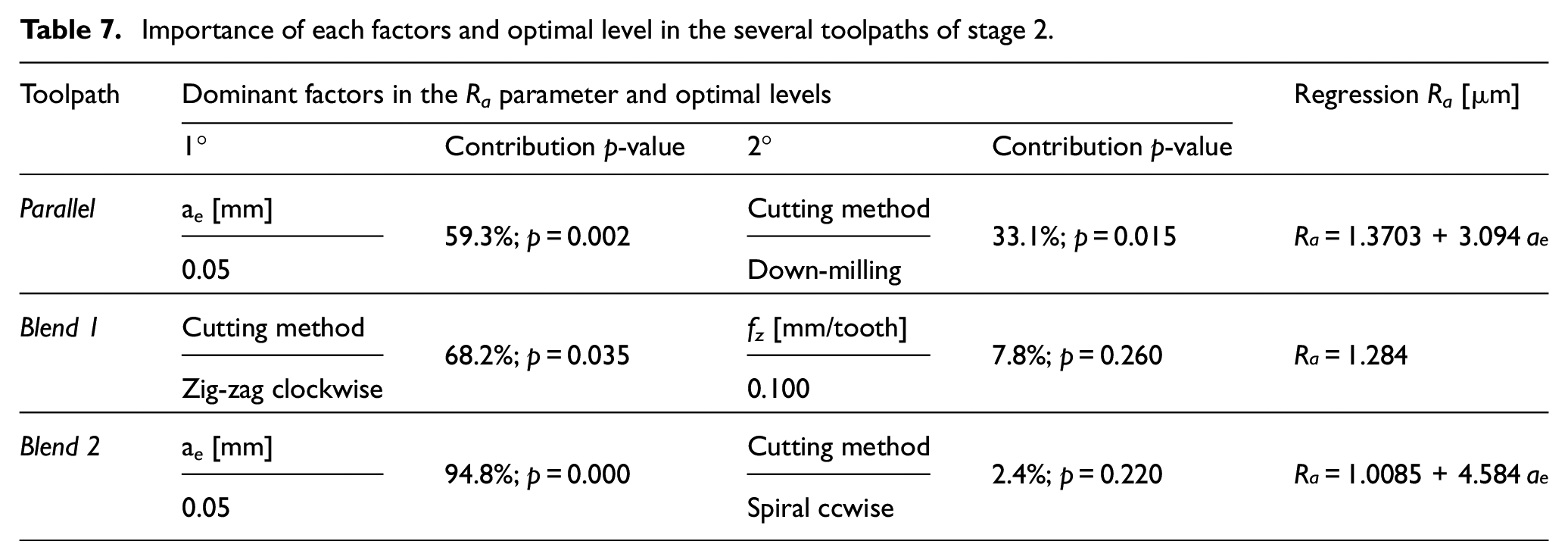
The response tables show that the a_e is the dominant factor in the Parallel and Blend 2 toolpaths, and the cutting method in the remaining trajectory. Table 7 summarises the ANOVA results, presenting each factor’s contribution to the R_a value, its significance level and its regression equation. With a 95% confidence interval (CI) and 5% significance level, in the Parallel toolpath, both factors are statistically significant justifying 59.3% (a_e) and 33.1% (cutting method) of the results, with the remaining 7.6% being allocated to error. With Blend 1 the f_z is statistically not significant, leaving the R_a constant in each level of the cutting method, the best being 1.28 µm at the zig-zag level. The last factor accounts for 68.2% of the results. The a_e factor, in the Blend 2 strategy, justifies almost the entire R_a variation (94.8% of variance explained), with the cutting method and their interaction not being statistically significant. Therefore, the error and other uncontrolled factors were smaller in this strategy, accounting for only 5.2%. Analysing the regression equations in Table 7, we conclude that the spiral toolpath is the one with the lowest R_a value for the same a_e, which at the limit leads to R_a = 1.0 µm. This conclusion was confirmed by new experiments whose results are shown below.

Table 7.

Importance of each factors and optimal level in the several toolpaths of stage 2.

Toolpath	Dominant factors in the R_a parameter and optimal levels				Regression R_a [µm]
Toolpath	1°	Contribution p-value	2°	Contribution p-value	Regression R_a [µm]
Parallel	a_e [mm]	59.3%; p = 0.002	Cutting method	33.1%; p = 0.015	R_a = 1.3703 + 3.094 a_e
	0.05	59.3%; p = 0.002	Down-milling	33.1%; p = 0.015	R_a = 1.3703 + 3.094 a_e
Blend 1	Cutting method	68.2%; p = 0.035	f_z [mm/tooth]	7.8%; p = 0.260	R_a = 1.284
	Zig-zag clockwise	68.2%; p = 0.035	0.100	7.8%; p = 0.260	R_a = 1.284
Blend 2	a_e [mm]	94.8%; p = 0.000	Cutting method	2.4%; p = 0.220	R_a = 1.0085 + 4.584 a_e
	0.05	94.8%; p = 0.000	Spiral ccwise	2.4%; p = 0.220	R_a = 1.0085 + 4.584 a_e

Confirmation tests

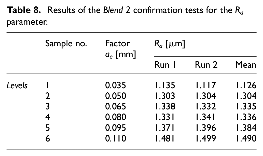
Table 8 shows the results of the confirmation tests for the best toolpath of the second stage, with the a_e factor varying in six levels and keeping the spiral ccwise level. Sample 1 (a_e = 0.035 mm) of the Blend 2 strategy presented a minimum value of R_a = 1.13 µm, confirming the trend of the optimal level. Figure 5(a) presents the linear regression and the lines relating to the 95% confidence and prediction intervals, showing that all the tests are comprised with in these ranges. The prediction equation of the second stage practically matches with the trend line of the confirmation tests, with a maximum difference of 2.4% (0.036 μm) for a_e = 0.11 mm within the domain, Figure 5(b). For the optimum level of the second stage (a_e = 0.050 mm), the R_a value was 1.30 μm, differing from the prediction by +5.4%, Figure 5(b). This level of the confirmation tests, through linear regression, has a +0.3% difference when compared to the previous prediction.

Table 8.

Results of the Blend 2 confirmation tests for the R_a parameter.

	Sample no.	Factora_e [mm]	R_a [µm]
			Run 1	Run 2	Mean
Levels	1	0.035	1.135	1.117	1.126
	2	0.050	1.303	1.304	1.304
	3	0.065	1.338	1.332	1.335
	4	0.080	1.331	1.341	1.336
	5	0.095	1.371	1.396	1.384
	6	0.110	1.481	1.499	1.490

Figure 5.

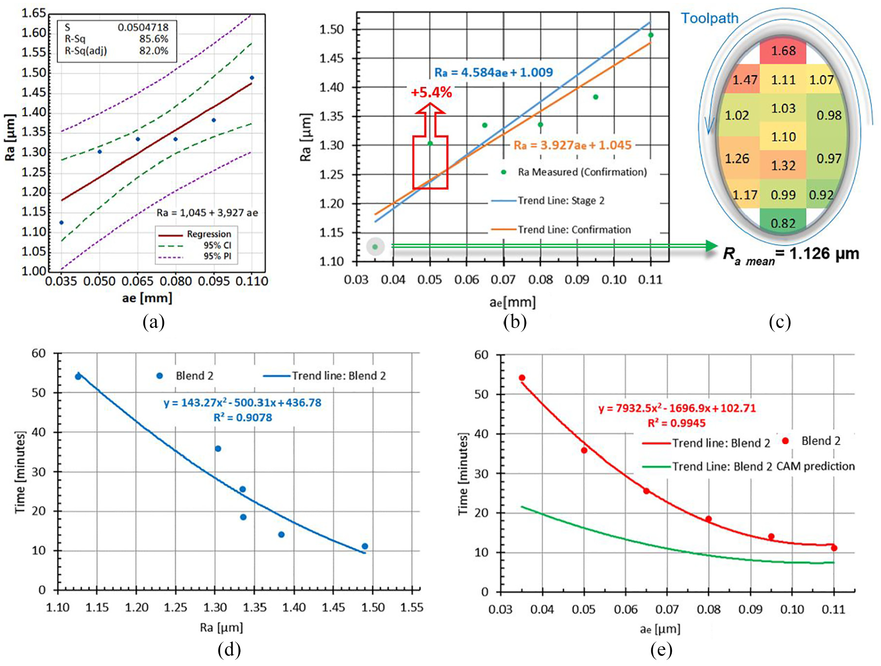
Blend 2 confirmation test: (a) fitted line for the R_a (a_e) parameter, with confidence and prediction intervals, (b) graphical comparison of the trend lines for stage 2 and for the confirmation, (c) mean values of R_a [μm], per zone (a_e = 0.035 mm) and time of the cavity finishing operations, as a function of (d) R_a and (e) a_e.

The mean result, by zone, for a_e = 0.035 mm is shown in Figure 5(c). The results of the second stage were confirmed with respect to the central zone of the cavity, obtaining R_a = 1.1 μm. In the confirmation test, as in the previous ones, some areas with R_a values lower than 1 μm were found, whose lowest value is 0.82 μm. The machining results of the right side of the cavity obtained a 20% better finish than the left side. This fact can be justified by the upward trajectory of the right half with the central strip having an intermediate value (6.5% better), as it contains both directions. In the lower half, it was also found that the R_a results are 13% better than on the upper half. In this case, the difference can be justified by the effective cutting speed, which is lower at the bottom, producing a smoother surface finish.

The ANOVA of the linear regression, presented in Table 9, confirmed that a_e is statistically significant, explaining about 85.6% of the results. This score is 9% lower than those of the second stage, but it accounts for a wider range. The standard error, S = 0.050 µm, is an acceptable value.

Table 9.

Analysis of variance of the regression, R_a versus a_e, for toolpath Blend 2 (confirmation).

Source	DF	SS Seq	Contribution	Adj SS	Adj MS	F-Value	p-Value
Regression	1	0.06072	85.63%	0.06072	0.060721	23.84	0.008
a_e [mm]	1	0.06072	85.63%	0.06072	0.060721	23.84	0.008
Error	4	0.01019	14.37%	0.01019	0.002547
Total	5	0.07091	100.00%
Model summary
S	R-sq	R-sq (adj)	PRESS	R-sq (pred)
0.0504718	85.63%	82.04%	0.0275335	61.17%
Regression equation
R_a [µm] = 1.0445 + 3.927*a_e [mm]

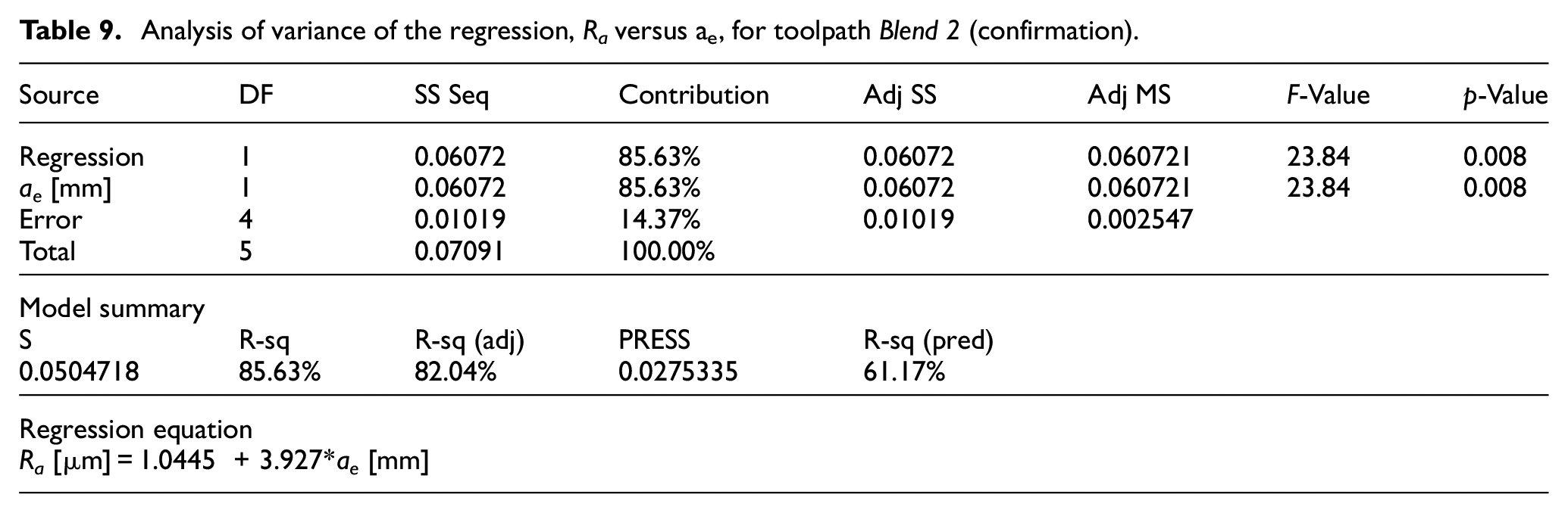
Figure 5(d) and (e) illustrates the time of the confirmation tests related to the R_a and a_e variables, respectively. Reducing the R_a from 1.30 to 1.13 μm requires twice the production time. There is a mismatch between the time provided by the Mastercam, marked with the green line on the graph, and the measured time (the red line). This difference is justified by the high number of points that builds the trajectory, and it is not possible to reach the programmed feed rate in the entire cavity. This phenomenon is most pronounced closer to the centre of the cavity. The time consumed can be significantly reduced if the protection of the CNC machine is deactivated against sudden acceleration/deceleration. With this change, a 34% reduction in the duration of the operation was achieved, when a_e = 0.035 mm. The impact in the remaining cases was smaller, at only 12% when a_e = 0.110 mm. This change was applied only during this toolpath, since during its execution there are no large or quick movements in the safety plane, making the existing movements more continuous and smoother.

The optimum set of control factors for the most effective toolpath, Blend 2, is: feed in spiral counter clockwise, reference point centred, a_e = 0.035 mm, f_z = 0.093 mm/tooth, with an outcome of R_a = 1.13 µm and time at 54 min.

Application – tibial insert

The toolpath and optimised parameters were applied in the execution of a tibial insert. In the manufacturing process, the fourth axis of the CNC was used. The rotation of this axis, allowed the machining of several planes with the same fixture. In the first phase of the process, the most important surfaces of the insert were machined (whose dimensional accuracy must be greater), including the two femoral cavities (to the left in Figure 6). After the first phase, the work piece was still attached laterally to the initial rod. After the removal of the tops, lateral contouring operations were performed, in a second fixture and using only three-axis machining in order to remove excess material, as shown in the centre of Figure 6. The resulting part of the entire manufacturing process is illustrated, in several directions, on the right, in Figure 6. In the femoral cavities a mean of R_a = 1.16 µm was achieved, similar to the values of the confirmation tests.

Figure 6.

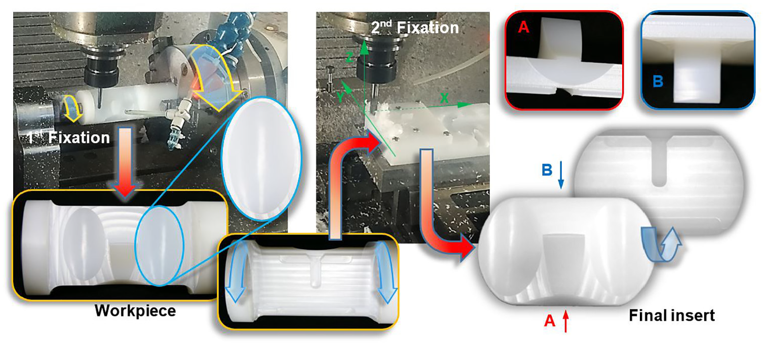
Machining the prototype of the knee prosthesis insert.

Conclusion

This work aimed to optimise high speed machining parameters to obtain the best possible surface finish of the femoral cavities of the tibial insert using a conventional ball end mill and a three-axes CNC machine. Several milling experiments of a UHMWPE test piece were implemented with the Taguchi method designed in two stages, with L9 arrays, and statistical analyses, like ANOVA. The optimal set of parameters and a prediction equation were validated by the confirmation milling experiments. The main conclusions of this work are as follows:

(i) ANOVA results determined the most important parameter on R_a to be the step over, at 59.3% and 94.8%, with Parallel and Blend 2 toolpaths, respectively, and the cutting method, at 68.2%, with Blend 1 strategy.

(ii) The Blend 2 strategy, leading to a continuous spiral toolpath, decreased the mean value of R_a for the cavities.

(iii) The optimal R_a values for the cutting method, feed rate, radial depth of cut, and chains were determined: feed in counter clockwise, 0.093 mm/tooth (1767 mm/min), 0.035 mm, and with the centre point and the elliptical contour of the cavity given as along and 3D, respectively.

(iv) The limitation of the 3 axes machining, to prevent abrasion in the central part of the cutter, can be overcome by tilting the work piece 45° relative to the tool axis, improving local values of R_a from 3.4 to 1.1 μm. All toolpaths benefited from this change.

(v) Under these conditions, the best mean R_a value, controlled in 15 zones and for two perpendicular directions, was 1.13 μm. The time spent in this finishing operation was 54 min. The R_a values can be predicted by the expression R_a [µm] = 1.04+3.93*a_e [mm], with a standard error of 0.05 µm and a_e∈[0.035, 0.110 mm], and

(vi) The obtained R_a values differ greatly from the theoretical values for flat surfaces machined by a ball end mill. For example, according to the theoretical equations for a_e = 0.12 mm, R_a is 0.6 μm and, experimentally, the value obtained was R_a = 2.0 μm, with Parallel toolpath.

(vii) The parameter statistically relevant in the linear regression is the radial depth of cut, with a contribution of approximately 86%, and the remaining percentage attributed to uncontrolled factors.

(viii) Using the obtained correlation, for lower radial depth of cut values and at the limit equal to zero, a R_a value close to 1.0 μm would be obtainable. However, this parameter selection would have a negative impact on runtime.

(ix) The production time was predicted by quadratic equations, as a function of the R_a and as function of a_e. Lowering the R_a from 1.30 to 1.13 μm increments the time by 93%. Decreasing the a_e from 0.05 to 0.035 mm raises the time by 70%.

(x) The spiral toolpath allows deactivating the protection of the CNC machine against sudden acceleration/deceleration, saving 12% to 34% of the finishing time, respectively for the highest (a_e = 0.110 mm) and the lowest (a_e = 0.035 mm) tested a_e value.

(xi) According to the confirmation test, the R_a measurements are with in the 95% confidence and prediction intervals.

The full execution of the tibial insert prototype, using strategy and the optimum set of cutting parameters and carried out with conventional tools, took approximately 2 h and 20 min, achieving similar values of roughness (R_a = 1.16 µm) in the femoral cavities, compared to those obtained in the test piece. This study shows that with conventional tools and three axes CNC machining it is possible to produce an UHMWPE tibial insert with a good roughness quality and with a thin thickness of 6 mm in the middle section of the femoral cavities.

Footnotes

Acknowledgements

The authors acknowledge Project No. 031556-FCT/02/SAICT/2017; FAMASI – Sustainable and intelligent manufacturing by machining, financed by the Foundation for Science and Technology (FCT), POCI, Portugal, in the scope of TEMA, Centre for Mechanical Technology and Automation – UID/EMS/00481/2013.

Declaration of conflicting interests

The author(s) declared no potential conflicts of interest with respect to the research, authorship, and/or publication of this article.

Funding

The author(s) received no financial support for the research, authorship, and/or publication of this article.

ORCID iD

Francisco J Lopes

References

Kurtz

SM.

Chapter 2-from ethylene gas to UHMWPE component: the Process of producing orthopedic implants. In: Kurtz

(ed.) UHMWPE biomaterials handbook. 3rd ed. Oxford: William Andrew Publishing, 2016, pp.7–20.

OECD. “Hip and knee replacement”. Health at a Glance 2017: OECD Indicators. Paris: OECD Publishing2017, pp.178–179.

Watters

Mather

RC 3rd

Browne

, et al. Analysis of procedure-related costs and proposed benefits of using patient-specific approach in total knee arthroplasty. J Surg Orth Adv 2011; 20: 112–116.

Macdonell

Browne

JA.

Procedure 40-methods of fixation in total knee arthroplasty. In: Miller

Browne

Cole

, et al. (eds) Operative techniques: knee surgery. 2nd ed. Philadelphia: Elsevier, 2018, pp.366–369.

Evans

Walker

Evans

, et al. How long does a knee replacement last? A systematic review and meta-analysis of case series and national registry reports with more than 15 years of follow-up. The Lancet 2019; 393: 655–663.

Panjwani

Mullaji

Doshi

, et al. Comparison of functional outcomes of computer-assisted vs conventional total knee arthroplasty: a systematic review and meta-analysis of high-quality, prospective studies. J Arthroplasty 2019; 34: 586–593.

Schroeder

Martin

In vivo tibial fit and rotational analysis of a customized, patient-specific TKA versus off-the-shelf TKA. J Knee Surg 2019; 32: 499–505.

X-D

Xiang

B-Y

Schotanus

MGM

, et al. CT-versus MRI-based patient-specific instrumentation for total knee arthroplasty: a systematic review and meta-analysis. Surg 2017; 15: 336–348.

Dirks

Bergmann

Mai

, et al. A prospective multicentric analysis of patient data and functional tests of standard knee prosthesis compared to individualized knee prosthesis implantation (NexGen CR vs. ConforMIS iTotal CR). Orthop J Sports Med 2018; 6: 2325967118S00033.

10.

Changhui

Aibing

Yongqiang

, et al. Customized UHMWPE tibial insert directly fabricated by selective laser sintering. Int J Adv Manuf Tech 2016; 85: 1217–1226.

11.

Malito

Arevalo

Kozak

, et al. Material properties of ultra-high molecular weight polyethylene: comparison of tension, compression, nano mechanics and micro structure across clinical formulations. J Mech Behavi Biomed Mater 2018; 83: 9–19.

12.

Zaribaf

Medical-grade ultra-high molecular weight polyethylene: past, current, and future. Mater Sci Technol 2018; 34(16): 1940–1953.

13.

Aldwell

Hanley

O’Donnell

GE.

Characterising the machining of biomedical grade polymers. Proc IMechE, Part B: J Engineering Manufacture 2014; 228: 1237–1251.

14.

Chakrabarty

Vashishtha

Leeder

Polyethylene in knee arthroplasty: a review. J Clin OrthopTrau 2015; 6: 108–112.

15.

Ollivier

Parratte

Flecher

, et al. The mobile-bearing TKA: is there still a place? Tech Ortho 2018; 33: 25–28.

16.

Van Hamersveld

Marang-Van

Mheen

Van Der Heide

HJL

, et al. Migration and clinical outcome of mobile-bearing versus fixed-bearing single-radius total knee arthroplasty. Acta Orthop 2018; 89: 190–196.

17.

Nowakowski

Vavken

Pagenstert

, et al. Chapter 8 – design, shape, and materials of total knee replacement. In: Hirschmann

Becker

(eds) The unhappy total knee replacement: a comprehensive review and management guide. Cham: Springer International Publishing, 2015 pp.85–97.

18.

Causero

Di Benedetto

Beltrame

, et al. Design evolution in total knee replacement: which is the future? Acta Biomed 2014; 85(Suppl 2): 5–19.

19.

Garabédian

Bigerelle

Najjar

, et al. Wear pattern on a retrieved total knee replacement: the “fourth body abrasion.” Biotribology 2017; 11: 29–43.

20.

Sharkey

Lichstein

Shen

, et al. Why are total knee arthroplasties failing today – has anything changed after 10 years? J Arthro 2014; 29: 1774–1778.

21.

Sava

Munteanu

Renault

, et al. Tribological analysis of UHMWPE tibial implants in unicompartmental knee replacements: from retrieved to invitro studies. Biotribology 2018; 13: 1–15.

22.

Varadarajan

Oral

Muratoglu

, et al. Why all tibial polyethylene bearings are not the same? Tech Ortho 2018; 33: 17–24.

23.

Popa

Wang

Descartes

, et al. Role of surface industrial finishing process of joint implant UHMWPE on their tribological behaviour. Appl Mech Mater 2014; 658: 465–470.

24.

Menezes

Kailas

SV.

Role of surface texture and roughness parameters on friction and transfer film formation when UHMWPE sliding against steel. Biosur Biotrib 2016; 2: 1–10.

25.

Wang

Jin

McEwen

HMJ

, et al. Microscopic asperity contact and deformation of ultra high molecular weight polyethylene bearing surfaces. Proc IMechE, Part H: J Engineering Medicine 2003; 217: 477–490.

26.

Guenther

Turgeon

Bohm

, et al. The biochemical characteristics of wear testing lubricants affect polyethylene wear in orthopaedic pin-on-disc testing. Proc IMechE, Part H: J Engineering Medicine 2015; 229: 77–90.

27.

Shintoku

Narita

Study on ball end milling of inclined surfaces for ultra high molecular weight polyethylene. Int J Auto Tech 2017; 11: 948–957.

28.

Dikshit

Puri

Maity

Analysis of cutting force coefficients in high-speed ball end milling at varying rotational speeds. Mach Sci Tech 2017; 21: 416–435.

29.

Kara

Öztürk

Comparison and optimization of PVD and CVD method on surface roughness and flank wear in hard-machining of DIN 1.2738 mold steel. Sen Rev 2019; 39: 24–33.

30.

Zhang

Huang

Chen

, et al. Experimental study of coverage constraint abrasive flow machining of titanium alloy artificial joint surface. Proc IMechE, Part B: J Engineering Manufacture 2019; 233: 2399–2409.

31.

Paschoalinoto

Bordinassi

Bortolussi

, et al. The effect of process parameters and cutting tool shape on residual stress of SAE52100 hard turned steel by high speed machining. Proc IMechE, Part B: J Engineering Manufacture. Epub ahead of print 25 June 2020. DOI: 10.1177/0954405420929788.

32.

Zhao

Zheng

, et al. Tool tip cutting specific energy prediction model and the influence of machining parameters and tool wear in milling. Proc IMechE, Part B: J Engineering Manufacture 2020; 234(10): 1346–1354.

33.

Quintana

Ciurana

Ribatallada

Surface roughness generation and material removal rate in ball end milling operations. Mater Manuf Proc 2010; 25: 386–398.

34.

Zhang

Sun

Swept surface-based approach to simulating surface topography in ball-end CNC milling. Int J Adv Manuf Tech 2018; 98: 107–118.

35.

Álvarez

Calleja

Arizmendi

, et al. Spiral bevel gears face roughness prediction produced by CNC end milling centers. Materials (Basel, Switzerland) 2018; 11: 1301.

36.

Saptaji

Gebremariam

Azhari

MABM

. Machining of biocompatible materials: a review. Int J Adv Manuf Tech 2018; 97: 2255–2292.

37.

Hazir

Erdinler

Koc

KH.

Optimization of CNC cutting parameters using design of experiment (DOE) and desirability function. J For Res 2018; 29: 1423–1434.

38.

Nghiep

Sarhan

AAD

Aoyama

Analysis of tool deflection errors in precision CNC end milling of aerospace Aluminum 6061-T6 alloy. Measurement 2018; 125: 476–495.

39.

Mersni

Boujelbene

Salem

, et al. Optimization of the surface roughness in ball end milling of titanium alloy Ti-6Al-4 V using the Taguchi Method. Procedia Manuf 2018; 20: 271–276.

40.

Lauro

Pereira

RBD

Brandão

, et al. Design of experiments – statistical and artificial intelligence analysis for the improvement of machining processes: a review. In: Davim

(ed.) Design of experiments in production engineering. Cham: Springer International Publishing, 2016, pp.89–107.

41.

Kara

Taguchi optimization of surface roughness and flank wear during the turning of DIN1.2344 tool steel. Mater Test 2017; 59: 903–908.

42.

Öztürk

Kara

Calculation and estimation of surface roughness and energy consumption in milling of 6061 alloy. Adv Mater Sci Eng 2020; 2020: 1–12.

43.

Chang

H-J

Chen

S-L

Lee

P-Y.

Using the direct cutting paths approach on aluminum alloy cone frustum part for evaluating a five-axis machine tool with Taguchi method. Proc IMechE, Part B: J Engineering Manufacture 2017; 231: 881–888.

44.

J-W

Jia

Z-Y

Wang

F-J

, et al. Spindle speed selection for high-speed milling of titanium alloy curved surface. Mater Manuf Process 2014; 29: 364–369.

45.

Volpato

de Amorim

JR.

A procedure for dealing with milling limitations in machined prototype tooling. Proc IMechE, Part B: J Engineering Manufacture 2011; 225: 2163–2176.

46.

Wang

Jiang

Tao

, et al. A new test part to identify performance of five-axis machine tool – part I: geometrical and kinematic characteristics of S part. Int J Adv Manuf Tech 2015; 79: 729–738.

47.

Wang

, et al. Geometric deviation reduction method for interpolated toolpath in five-axis flank milling of the S-shaped test piece. Proc IMechE, Part B: J Engineering Manufacture 2019; 234: 910–919.

Toolpath and machining parameters optimisation of the cavities of a knee prosthesis tibial insert

Abstract

Keywords

Introduction

Materials and methods

First stage of testing

Second stage of tests

Confirmation experiments

Test-part definition

Simulation and machining

Evaluation of the surface quality of the cavity

Results and discussion

First stage of testing

Second stage of testing

Confirmation tests

Application – tibial insert

Conclusion

Footnotes

Acknowledgements

Declaration of conflicting interests

Funding

ORCID iD

References