Sage Journals: Discover world-class research

Abstract

Due to the latest advancements in monitoring technologies, interest in the possibility of early-detection of quality issues in components has grown considerably in the manufacturing industry. However, implementation of such techniques has been limited outside of the research environment due to the more demanding scenarios posed by production environments. This paper proposes a method of assessing the health of a machining process and the machine tool itself by applying a range of machine learning (ML) techniques to sensor data. The aim of this work is not to provide complete diagnosis of a condition, but to provide a rapid indication that the machine tool or process has changed beyond acceptable limits; making for a more realistic solution for production environments. Prior research by the authors found good visibility of simulated failure modes in a number of machining operations and machine tool fingerprint routines, through the defined sensor suite. The current research set out to utilise this system, and streamline the test procedure to obtain a large dataset to test ML techniques upon. Various supervised and unsupervised ML techniques were implemented using a range of features extracted from the raw sensor signals, principal component analysis and continuous wavelet transform. The latter were classified using convolutional neural networks (CNN); both custom-made networks, and pre-trained networks through transfer learning. The detection and classification accuracies of the simulated failure modes across all classical ML and CNN techniques tested were promising, with all approaching 100% under certain conditions.

Keywords

Digital manufacturing optimisation machine learning machine tool fault detection fault classification fingerprint routine process monitoring machining

Introduction

Techniques for process monitoring of machining operations through sensor signals are well-established in the literature.¹ Many solutions utilising such techniques have now been commercialised and are available to industry, for example, Marposs ARTIS,²Nordmann Tool Monitoring,³ and Sandvik CoroPlus.⁴ These commercial systems are often focussed on detecting tool breakages, collisions, or other catastrophic failures, through comparing signal levels to static limits or signal trending. Although useful, more advanced techniques of process monitoring have been proven to be able to provide significantly richer information about the process.

Traditional time-domain statistical features (i.e. RMS, kurtosis, standard deviation, mean and skewness) have been commonly used for detection and prediction of faults and errors in machinery.⁵ For example, researchers like D’Emilia et al.⁶ and Uhlmann et al.⁷ extracted time domain features from acoustic emissions and vibration signals; and applied machine learning (ML) techniques, such as support vector machine, Bayes and nearest-neighbour, to classify failure modes on rotational equipment. Similarly, Nam et al.⁸ utilised a non-linear support vector machine on accelerometer and acoustic emission signal RMS values to detect a fault state during an additive manufacturing process. This method achieved up to 100% accuracy when detecting issues caused by an uneven print bed of the fused deposition model machine under test.

Such techniques involving time-domain features have also been demonstrated successfully with machining operations. For example, Kaya et al.⁹ trained a support vector machine to predict tool wear from time domain features extracted from a combination of force, vibration and acoustic emissions signals from milling operations. The real-time capability of ML techniques for process monitoring has also been demonstrated by Ma et al.,¹⁰ who were able to compensate for thermal errors in a high-speed spindle using a back propagation neural network analysing signals from temperature and eddy current sensors. The system was found to be able to increase radial and axial accuracy of the jig borer under test by over 80%. Segreto et al.¹¹ also utilised a feed-forward back-propagation neural network to classify the type of chip formation in turning, with features from force and displacement signals selected through principal component analysis (PCA).

Furthermore, time-frequency domain features, such as wavelet transform techniques have also been widely used for monitoring purposes. For instance, Sevilla-Camacho et al.¹² used continuous wavelet transforms (CWT) to illustrate the differences in vibration signals from ‘healthy’ and ‘damaged’ cutting tools. Likewise, Wang et al.^13,14 used wavelet transformations in the form of scalograms to train a convolutional neural network (CNN) to classify a number of failure modes in a bearings system and a gear box, respectively. Guo et al.¹⁵ successfully employed a long short-term memory network to analyse features extracted through wavelet packet decomposition of in-process acoustic emission signals for the assessment of grinding wheel condition. And to increase the robustness of chatter identification in thin-walled milling processes, an issue caused by highly dynamic and complex workpiece-tool interactions, Wang et al.¹⁶ developed an adaptive time-frequency domain feature selection process. In conjunction with a decision tree model, the authors were able to detect chatter with an accuracy of 92.42%.

If in-process signal data could be used to validate machining operations, an ‘inspection by exception’ approach could be adopted. This is defined by the authors as a regime in which inspection of components only takes place if a deviation from normal process envelopes are detected, or the process cannot be validated for any other reason. Such a methodology would be invaluable in industry, where there is interest in reducing the requirement for lengthy component inspection procedures, which currently represents a significant bottleneck in manufacturing, as demonstrated by Tiwari et al.¹⁷ It also supports the progress towards a zero defect manufacturing (ZDM) strategy; particularly for the middle of manufacturing life fault detection, as defined by Psarommatis et al.¹⁸ in their ZDM state-of-the-art review. The authors also identified a significant gap in beginning of manufacturing life ZDM strategies; which, amongst other things, includes gauging machine health prior to the manufacturing process.

Previous research conducted by Dominguez-Caballero et al.¹⁹ represented a first step in developing a combined system for machine and process health monitoring that utilised advanced signal analysis techniques. The authors successfully designed and tested a machine and process health monitoring system that utilised a shared sensor suite. The machine health was gauged using a repeatable ‘fingerprint routine’, which was designed to include isolated and combined movements of the X-, Y- and Z-axes, as well as rotation of the spindle; whilst the process monitoring was conducted during the machining of nine test vehicles in Ti-6Al-4V, which were based on the ‘circle, diamond, square’ test defined in BS ISO 10791-7-2014.²⁰ The analysis of the data captured, though limited in terms of the number of analysis techniques tested, was considered successful – particularly in the use of a novel comparative CWT method that was devised during this research.

The current research was therefore proposed to expand on the analysis techniques developed, with the major aim of utilising ML to detect and categorise faults. This provided the opportunity for additional machining trials to be undertaken to produce the significantly higher number of repeats needed for training ML. The ML techniques investigated included a range of classical ML techniques, such as PCA, classification and clustering; as well as deep learning techniques, in the form of custom-made CNNs and transfer learning of existing CNNs (AlexNet, GoogLeNet and ResNet-18).

The remainder of this paper includes descriptions of the equipment and experimental method employed during the machining trials (Sections 2 and 3); the signal processing and ML techniques tested (Section 4); a summary of the results and discussion from the analysis stage (Section 5); and finally, the conclusions drawn, including suggestions for further research (Section 6).

Experimental setup

The machining trials in this research were conducted on a DMG Mori DMU 40 eVo linear 5-axis milling machine tool. One accelerometer (PCB 356A02) was mounted on the spindle column of the machine tool, and another (PCB 604B31) was mounted on the machine bed, underneath the workpiece, incorporated into a steel plate. Both accelerometers are tri-axial. The setup is illustrated in Figure 1. A power monitoring device (Load Controls PPC-3) was also fitted to the spindle motor power supply cables. This provided a total of seven signals that could be recorded simultaneously.

Figure 1.

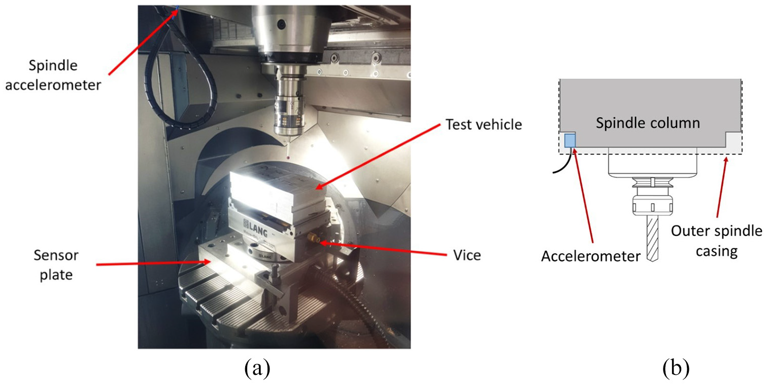
Illustration of (a) the machining configuration and (b) the spindle accelerometer location.

The signals from these sensors were captured and recorded using National Instruments (NI) LabVIEW software via a NI cDAQ-9718 with three modules installed: two NI-9234 modules sampling the vibration signals at 51.2 kHz; and one NI-9223 module sampling the power signal at 1 kHz.

The material used in this research was Al6082 cut into blocks with dimensions 200 × 120 × 85 mm. The tool used for the cutting trials was a Sandvik 392.410EH-63 25 105 adapter for carbide heads paired with a CoroMill 316-25SM345-25000A H10F three-flute 25 mm diameter solid carbide head (Figure 2(a)).

Figure 2.

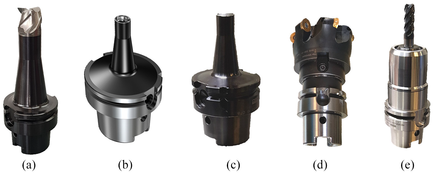
Tools used for: (a) the cutting trials; and the testing of the fingerprint routine, (b) baseline tool, (c) unbalanced tool (with sheared carbide head present), (d) linear axis heavy tool (face mill) and (e) spindle rotation heavy tool (chucked end mill).

For the fingerprint routine testing, tools were selected as follows. To allow a direct comparison between the baseline tool and an unbalanced tool, two identical tool holders (Figure 2(b) and (c)) were used. The baseline tool comprised of the adapter for carbide heads (no carbide head inserted); but the unbalanced tool contained the remaining thread of a carbide head that had previously been sheared off. The two adapters were almost identical in mass (0.77 kg), but the adapter with the carbide head remnant had a measurably higher imbalance (4.0 gmm) than the empty adapter (0.1 gmm).

For testing the effect of the tooling mass on the linear axis motions, a large face mill tool (Figure 2(d)) was ideal due to its considerably larger mass (3.51 kg, including indexable tools and tool holder) than the baseline tool. For testing the effect of the tooling mass on the spindle rotation, a chucked end mill (Figure 2(e)) around two times heavier than the baseline tool (1.66 kg, including tool and tool holder, compared to 0.77 kg), was opted for as this could be run at higher rotational speeds than the face mill. Hence a combination of tools were used for the heavy tool depending on the fingerprint routine being run.

Experimental method

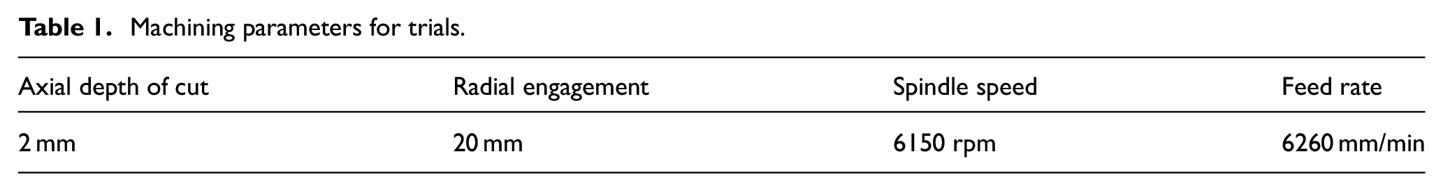
The method undertaken for the experimental tests utilised simplified operations from those in the previous research.¹⁹ The machining trials consisted of straight up-milling face cuts with the 25 mm end mill described in Section 2, with the machining parameters listed in Table 1. These parameters allowed six machining passes per layer of material, with 35 layers of material per block of aluminium; giving a total of 210 datasets per workpiece. A total of ten workpieces were machined during the trials, with various defects applied, as described in Section 3.1.

Table 1.

Machining parameters for trials.

Axial depth of cut	Radial engagement	Spindle speed	Feed rate
2 mm	20 mm	6150 rpm	6260 mm/min

The fingerprint routine consisted of only two sub-routines: the motion from a central location to each extreme and back along only the X-axis at a feed rate of 40,000 mm/min; and spindle rotation at 12,000 rpm with a dwell for 3 s once up to speed.

Failure mode and defect physical simulation

The methodology used for physically simulating machine tool failure modes and part defects was devised in the previous research, and so the rationale and finer details can be found in the paper by Dominguez-Caballero et al.¹⁹ Instead, a brief overview of the simulated failure modes and defects tested in this research is presented here.

The simulated machining defects consisted of:

Baseline [two workpieces affected] – No failure mode.

Misalignment [four workpieces affected] – Tilt machine tool’s bed by A: 0.27°, B: 0.27°, C: 0.32°.

Surface cracks [two workpieces affected] – Drill 1.84 mm diameter bores into the part, on the cutting path, before recorded trials.

Tool wear [two workpieces affected] – Wear the cutting tool severely before recorded trials (a fresh tool was used for each of the other test vehicles).

It should be noted that during misalignment affected operations, after a complete single layer had been machined, the subsequent layers would no longer suffer from a tilt in the horizontal plane. To combat this, before the start of each layer, the bed was tilted so that odd numbered layers had a rotation of A: 0.27°, B: 0.27°, C: 0.32°, whilst the even numbered layers had A: 0°, B: 0°, C: 0°; resulting in a tilt of the face that was about to be machined for every layer. Please note that although the machine tool possesses only two rotational axes (both acting upon the machining table), the B-axis is not orthogonal to the machine coordinates; hence an equivalent rotation expressed in terms of orthodox A-, B- and C-axis rotations is presented. This particular rotation allowed not only a variation in axial depth of cut of 0.94 mm to be experienced through any one pass, but also an increase in the initial depth of cut of 0.09 mm between the subsequent six passes of each layer; enriching the variance of the data set.

The simulated machine tool failure modes consisted of:

Baseline– No failure mode.

Heavy tool– Load a significantly heavier tool than the baseline tool (as described in Section 2).

Unbalanced– Load a tool that has a lower balancing classification that the baseline tool (as described in Section 2).

Feedrate-adjusted– Conduct the fingerprint routine with a set of marginally reduced feed rate and spindle speed overrides (corresponding to an even spread of 6-10% reduction).

Both of the fingerprint sub-routines (X-axis travel and spindle rotation) were conducted a total of 500 times whilst under the influence of each of the failure modes. However, the unbalanced failure mode was omitted for the linear axis routine, as an unbalanced tool (at this magnitude) would have no effect on axis motion.

Analysis methodology

Data processing

Before signal data could be analysed by the ML techniques, a number of data processing steps needed to be taken to make the format of the data appropriate. The following sub-sections outline this process.

Feature extraction

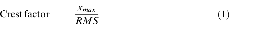
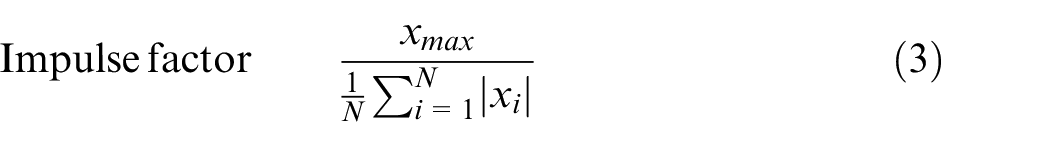
The classical ML techniques employed in this research all required a number of single-value features, commonly known as ‘predictors’, to be calculated for each of the signals. A table for each routine was then constructed that included all of the predictors from each of the runs/passes. There were 15 time-domain predictors selected and used in this research, based upon the recommendations of Ali et al.⁵ for the diagnosis of wind turbine bearings. These included features commonly used in signal analysis: mean, standard deviation, root mean squared (RMS), kurtosis, skewness and peak-to-peak; as well as those less commonly used: crest factor, shape factor, impulse factor, margin factor and energy, which are defined in equation (1)–(5):

Crest factor \frac{x_{\max}}{RMS}

(1)

Shape factor \frac{RMS}{\frac{1}{N} \sum_{i = 1}^{N} | x_{i} |}

(2)

Impulse factor \frac{x_{\max}}{\frac{1}{N} \sum_{i = 1}^{N} | x_{i} |}

(3)

Margin factor \frac{x_{\max}}{{(\frac{1}{N} \sum_{i = 1}^{N} | x_{i} |)}^{2}}

(4)

Energy \frac{1}{N} \sum_{i = 1}^{N} {x_{i}}^{2}

(5)

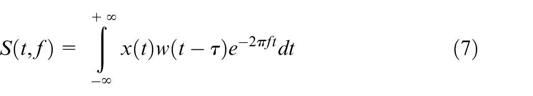
Spectral kurtosis is also known to be useful in prognosis applications,²¹ hence the spectral kurtosis, $K (f)$ (equation (6)), was produced for each signal. The mean, standard deviation, skewness and kurtosis of the spectral kurtosis were then also calculated.

Spectral kurtosis, K (f) = \frac{〈 {| S (t, f) |}^{4} 〉}{{〈 {| S (t, f) |}^{2} 〉}^{2}} - 2

(6)

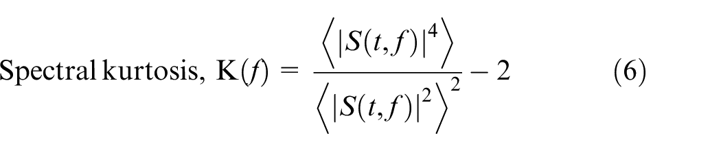
where, $S (t, f)$ is the short-time Fourier transform:

S (t, f) = \int_{- \infty}^{+ \infty} x (t) w (t - τ) e^{- 2 π ft} dt

(7)

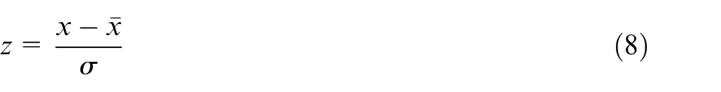
This gave a total of 15 predictors from each signal, and so, depending on the number of signals recorded for each routine/cut (up to six acceleration signals and one power signal), there were up to 105 predictors for a single observation. It should also be noted that all the extracted predictors were then normalised (using the ‘standard score’ method, shown in equation (8)) to ensure that the relative scales did not influence the ML techniques.

z = \frac{x - \bar{x}}{σ}

(8)

Continuous wavelet transform and filtering

The next step in the data preparation was to conduct CWT on all of the signals, producing the raw scalogram for each. The scalogram filtering process used in this research was developed and defined in¹⁹ and is summarised in the following steps, and illustrated in Figure 3:

A subset of the baseline scalograms are concatenated into a three-dimensional matrix.

Two two-dimensional matrices, one containing the average values, the other containing standard deviation, are calculated element-wise from the concatenated matrix.

The test scalogram is then subtracted from the average to produce an output scalogram, that is, the difference between the expected signal and actual signal.

To account for the inherent variance in the baseline signals, the output scalogram is then filtered using the standard deviation matrix to produce the resulting signal.

Steps 1 and 2 were repeated to produce the average scalogram and standard deviation matrix for each routine. Steps 3 and 4 could then be repeated for each of the full set of raw scalograms, producing a corresponding set of filtered scalograms.

Figure 3.

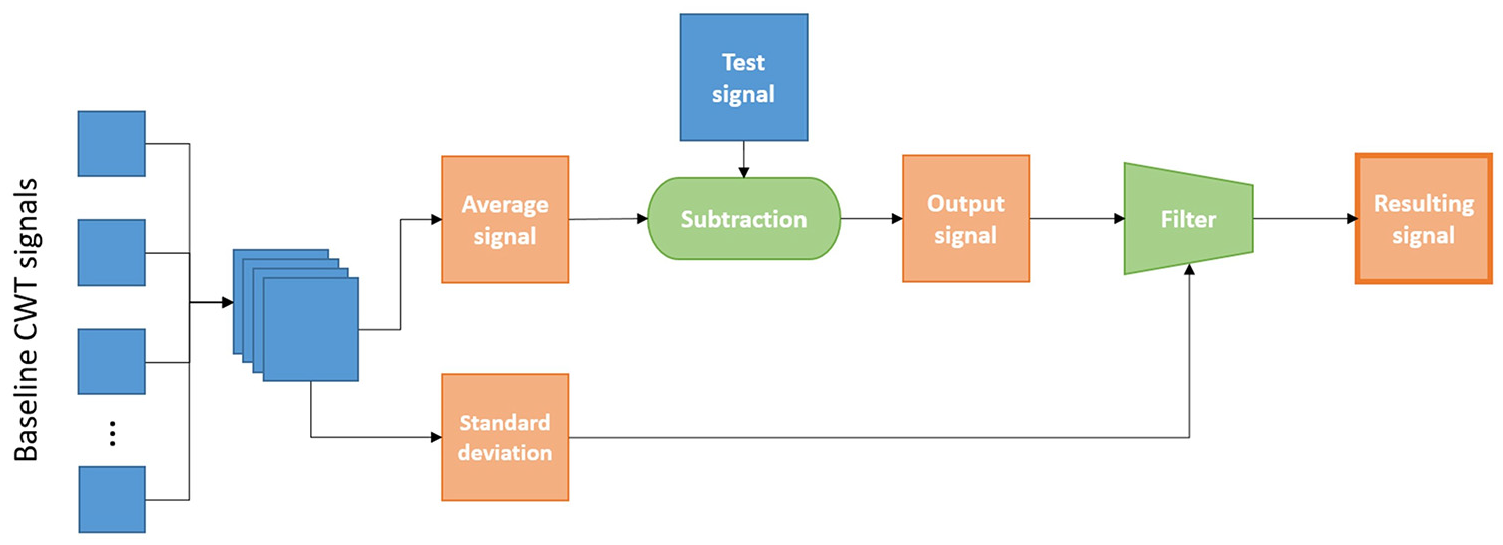
A chart to illustrate the technique developed for comparing the output from CWTs.¹⁹

An example of the resulting scalograms from this process is provided in Figure 4. The baseline average scalogram (Figure 4(a)) shows the nominal signal expected from a ‘good’ routine. The filtered scalograms highlight the deviations from the baseline average in the signals recorded during a repeated baseline test (Figure 4(b)), and a heavy tool test (Figure 4(c)). This illustrates that if a routine is run normally, there should be minimal signal in the resultant scalogram; whereas a routine that has been affected by some failure mode will exhibit significant signal in the resultant scalogram.

Figure 4.

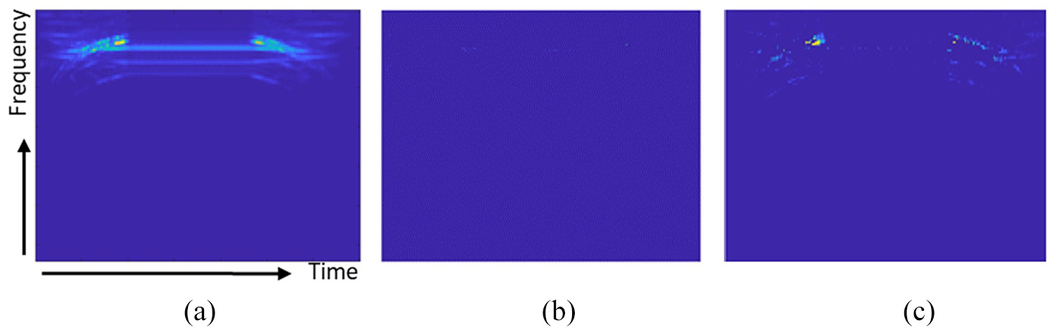
An example of: (a) the baseline average scalogram; and resultant filtered scalograms from, (b) a baseline test and (c) a heavy tool failure mode test for the 12,000 rpm spindle rotation fingerprint routine.

Image composition and resizing

To improve the image processing tasks and reduce computing time, the scalogram images were cropped and resized to 300 × 300 pixels. An image composition technique was developed to increase the number of images per failure mode. This technique consisted of generating up to three additional images from the original picture. The first composed image consisted of a horizontally flipped version of the original image. For the second and third images, the original image was cropped into two halves, keeping one half, then flipping it and attaching it to the original half in its two possible combinations: original half + flipped-half, and flipped-half + original half.

For the fingerprint routine tests, it was deemed that the composition techniques would have changed the nature of the signals. It was therefore decided that the total of 500 tests for each failure mode would be preserved, and so the ML techniques could be tested on a smaller number of repeats.

Machine learning techniques

Numerous types of classical ML were tested, which can be broken down into two main categories: supervised and unsupervised learning. Table 2 gives a brief description of each of the techniques tested.

Table 2.

Summary of the ML techniques tested.

	Subset of ML	Technique
Supervised	Classification	k-Nearest neighbour
		Naive Bayes
		Classification/ decision tree
		Multiclass support vectormachine
		Classification ensemble
	Deep learning	Convolutional neuralnetwork
Unsupervised	Dimensionalityreduction	Principal componentanalysis
	Clustering	k-Means clustering
		Gaussian mixture model(GMM)
		Hierarchical clustering

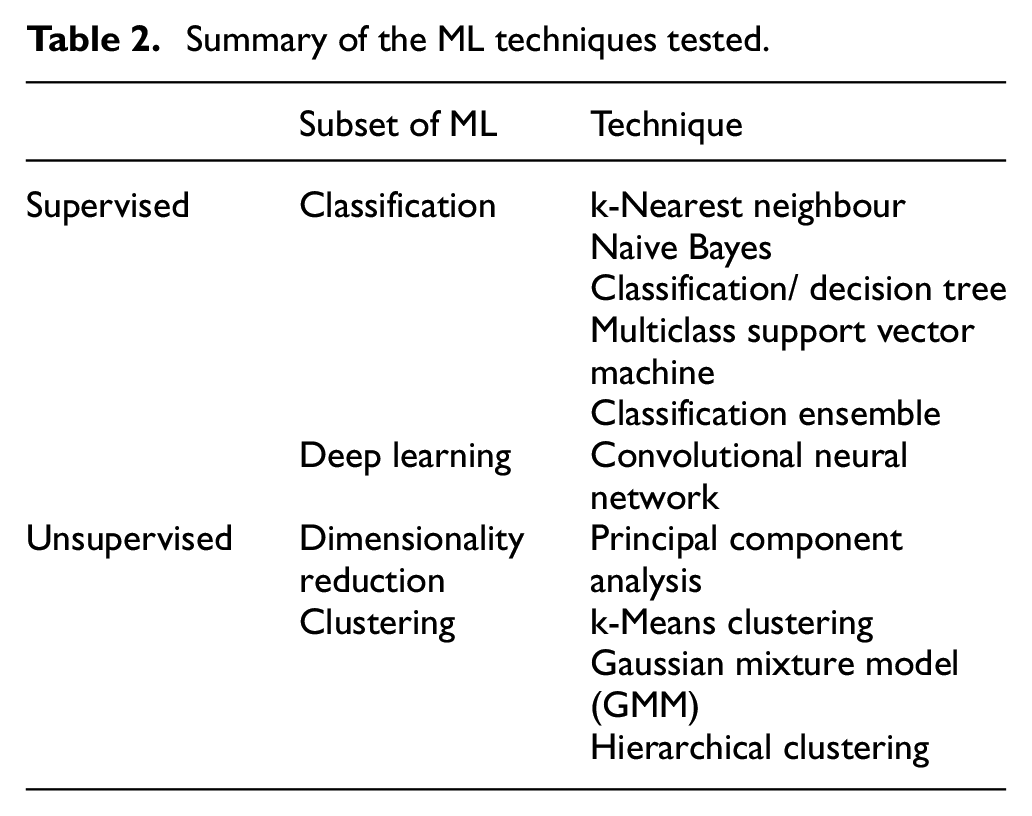
To gauge the effectiveness of each of the techniques the Rand index, a technique that measures similarity between two sets of clustering of the same data²² (i.e. actual vs predicted categories), was employed. This was used as it allows a direct comparison of results from the supervised techniques with the unsupervised techniques; whose accuracies cannot be gauged using traditional methods.

Classical machine learning

All five classification techniques tested were supervised; meaning they required a fully labelled training data set to be trained upon, and a set of unseen test data on which their accuracies could be tested. In this case, a 65:35 split was used to partition the data contained in the feature tables into training and testing data, respectively. The clustering techniques do not require this partitioning, and so were tested with the full datasets.

To give the greatest chance of success, the classical ML techniques were initially tested on the full set of features extracted. However, to make such techniques appropriate for a commercial system, they need to be able to run as close to real-time as possible. It is therefore advantageous to minimise the number of features analysed, thereby reducing the computational effort required for the analysis. However, reducing the number of features for analysis whilst still retaining sufficient information to successfully distinguish between failure modes is not trivial.

To assist with feature down-selection, PCA was used. PCA can be used to approximate a complex data set represented in N-dimensional space (in this case, N being the number of features), into a lower k-dimensional space, where k represents the number of principal components (PCs). Each PC is a weighted combination of the original features that produce a new set of orthogonal dimensions, where PC1 explains the largest proportion of the variation in the data, PC2 explains the next largest proportion of variation, and so on. Using this method, a data set with a high number of original features can often be approximated reasonably well with only two or three PCs.²³

Using PCA in combination with ML has been demonstrated as a successful technique for classification applications in the literature.¹¹ However, as PCA is a form of feature extraction, a large proportion of the original features are still required to calculate the first (in this case) three PCs. Therefore, PCA alone is not effective in reducing the number of features required, only in simplifying the interpretation of the results. To reduce the number of features, the weights of each feature’s contribution to each of the top three PCs were examined. A single feature was then selected to represent each PC, based on its weight and orthogonality to the other two features. The classical ML techniques, were then trained and tested again on only these reduced features to ascertain if they could still be effective when presented with a minimal data set.

Convolutional neural networks structures and parameters

Two custom-made networks were created and their accuracy and performance were compared with already existing networks. A defined procedure for selecting the structure, parameters and hyperparameter for a custom-made CNN could not be identified – this challenge has been seen before by other researchers.²⁴ Instead, a trial-and-error approach was adopted, until the CNNs could attain optimal level of accuracy inside a reasonable timeframe. This resulted in two different networks, each with a different structure; one optimised for vibration signals, the other optimised for power signals. The structure of these two custom-made networks is shown in Figure 5.

Figure 5.

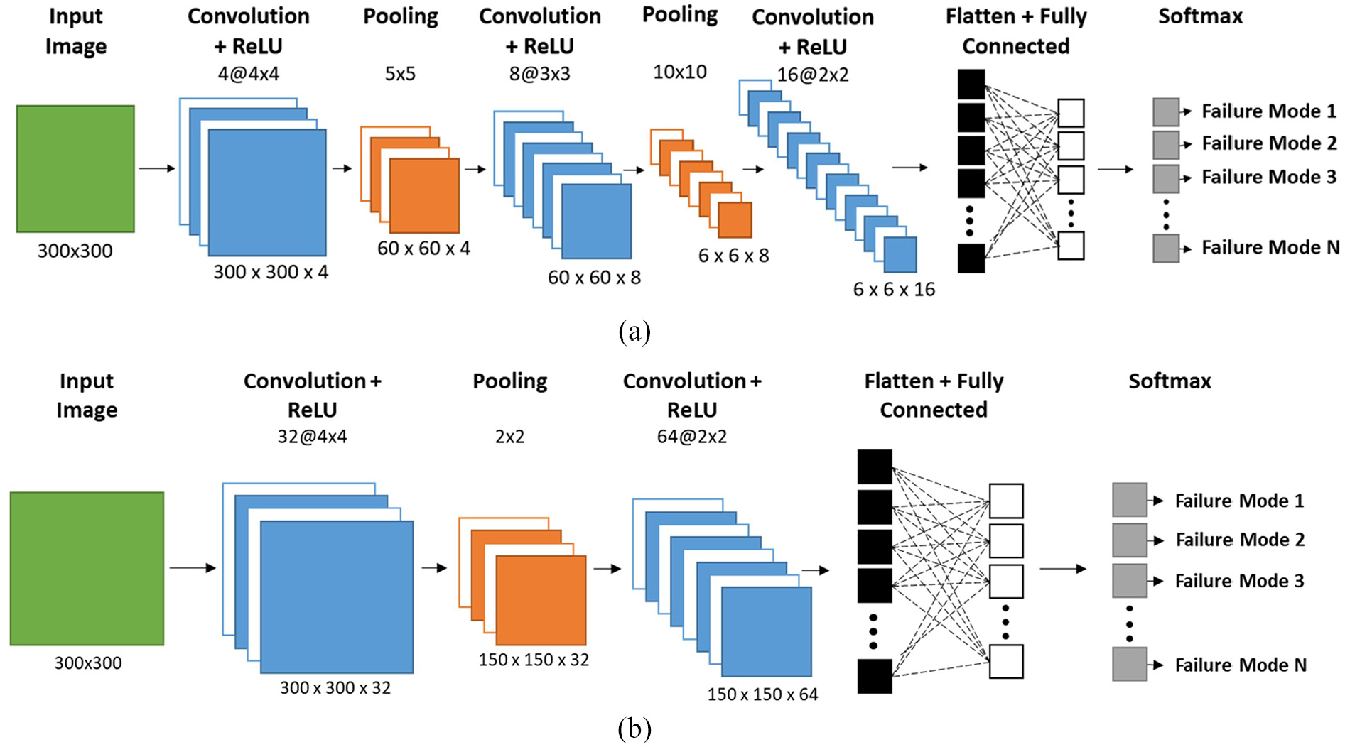
Custom-made CNN structures for: (a) vibration signals and (b) power signals.

The three pre-existing networks, AlexNet, GoogLeNet and ResNet-18, were tested using ‘transfer learning’. The structure of these networks is significantly more complex than the custom-made networks, (example provided in Figure 6), as they were originally designed to classify images of around 1000 categories, such as flowers, cars, dogs, etc. These therefore need re-training through transfer learning to make them proficient in categorising the CWT scalograms.

Figure 6.

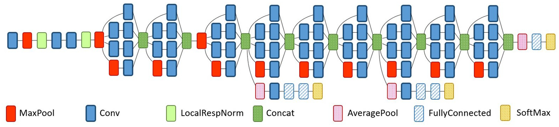
GoogLeNet CNN structure.²⁵

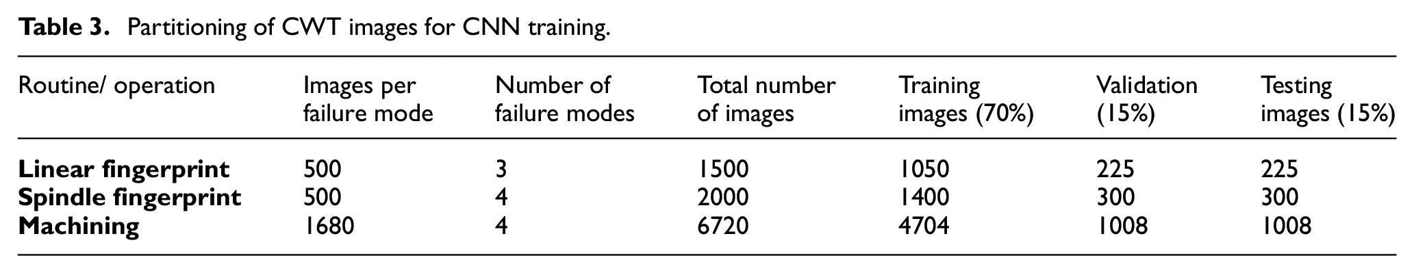
For the analysis of the CWT scalograms, the scalogram images were partitioned into training, validation and testing datasets; splitting the images as per common practice into 70%, 15% and 15%, respectively. The breakdown of the partitioning for each sensor signal for the fingerprint routines and the machining trials can be seen in Table 3. For training tasks, 20 epochs, with mini-batches of 32 images per iteration, were chosen. The testing dataset was then used to provide a final value of the performance of the CNN.

Table 3.

Partitioning of CWT images for CNN training.

Routine/ operation	Images perfailure mode	Number offailure modes	Total numberof images	Trainingimages (70%)	Validation(15%)	Testing images (15%)
Linear fingerprint	500	3	1500	1050	225	225
Spindle fingerprint	500	4	2000	1400	300	300
Machining	1680	4	6720	4704	1008	1008

Results and discussion

A significant number of charts and graphs were produced during the analysis stage, however, these are far too numerous to be included in this paper. Instead, what is presented in this section is a selection of the charts and graphs produced, for example purposes; along with the Rand index from each test to provide an overall comparison of the techniques employed.

Classical machine learning

Principal component analysis and feature reduction

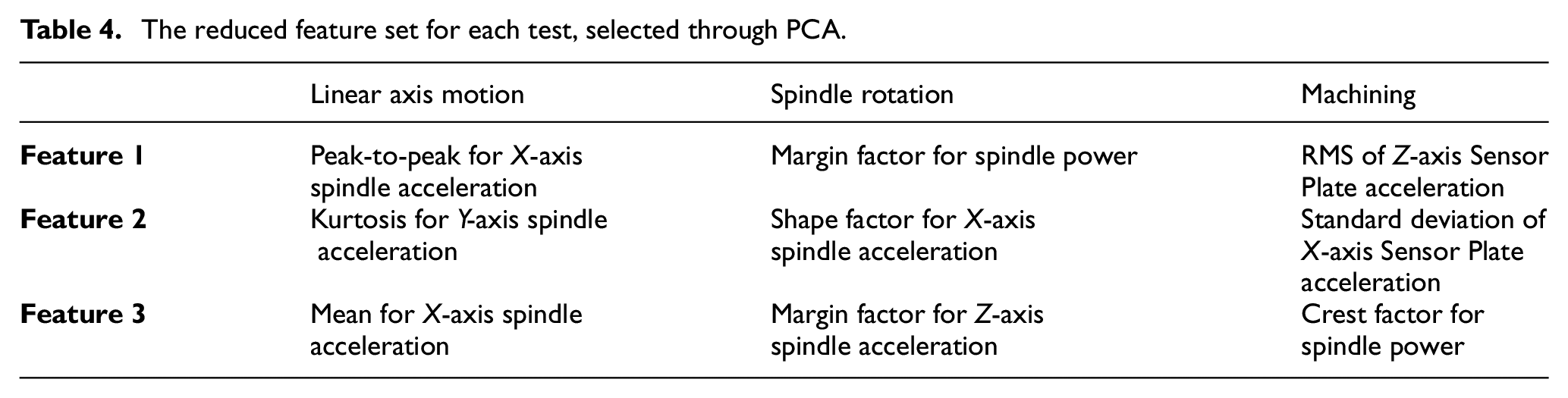
As explained in Section 4.2.1 there was a desire to investigate the effectiveness of utilising the full feature set for training and testing the ML techniques against using a greatly reduced number of features. To this end, PCA was utilised to help identify suitable features for the feature reduction. This feature reduction process was conducted using the method outlined in Section 4.2.1, for each fingerprint routine and machining operation separately. The features selected for each are given in Table 4.

Table 4.

The reduced feature set for each test, selected through PCA.

	Linear axis motion	Spindle rotation	Machining
Feature 1	Peak-to-peak for X-axis spindle acceleration	Margin factor for spindle power	RMS of Z-axis SensorPlate acceleration
Feature 2	Kurtosis for Y-axis spindle acceleration	Shape factor for X-axis spindle acceleration	Standard deviation ofX-axis Sensor Plateacceleration
Feature 3	Mean for X-axis spindle acceleration	Margin factor for Z-axisspindle acceleration	Crest factor for spindle power

Figures 7 –9 compare the actual groupings of the failure modes/faults (highlighted by different markers) for all three routines when using the first three PCs, and the top three selected features. It can be seen that, although they appear differently when plotted, the groupings are still distinct when plotted against the three features.

Figure 7.

The linear axis motion fingerprint routine data plotted against: (a) the first three PCs (PC1, PC2 and PC3) and (b) the three selected features.

Figure 8.

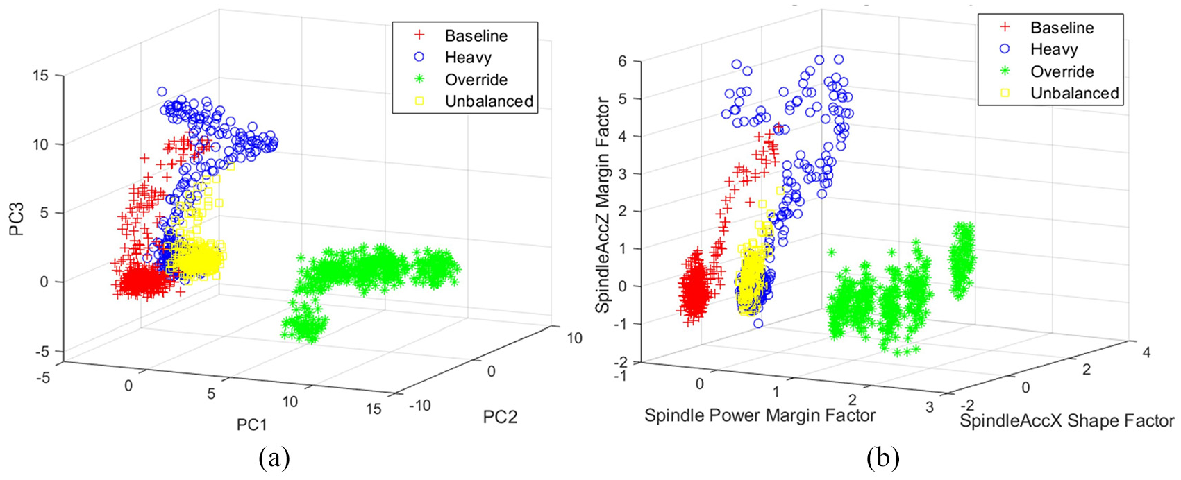
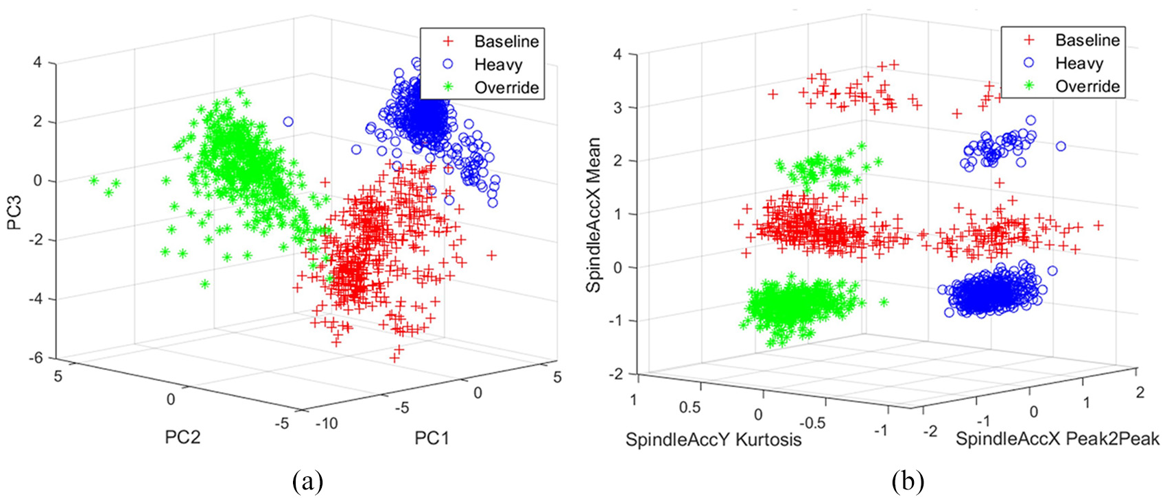
The spindle rotation fingerprint routine data plotted against: (a) the first three PCs (PC1, PC2 and PC3) and (b) the three selected features.

Figure 9.

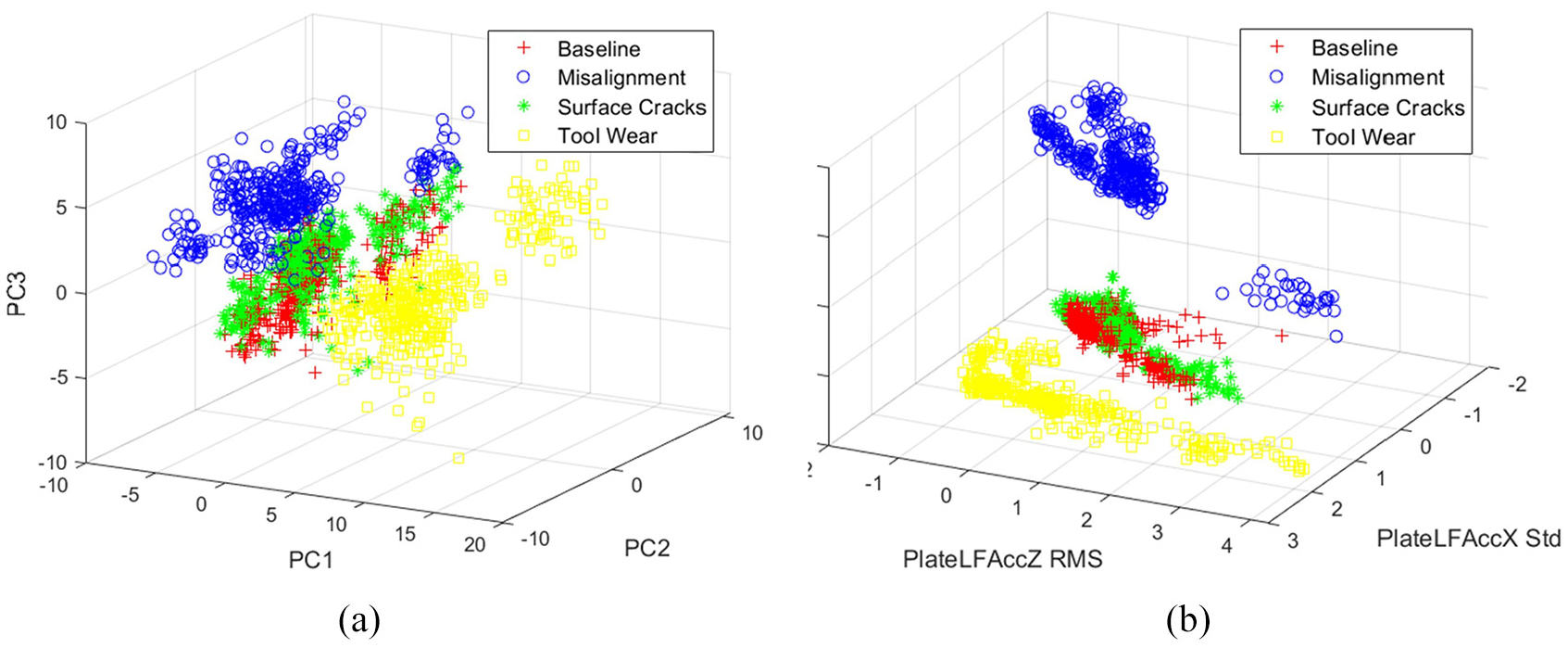
The machining data plotted against: (a) the first three PCs (PC1, PC2 and PC3) and (b) the three selected features.

Classification

The classification techniques were all trained and tested for each of the routines with both the full feature sets, and the reduced feature sets defined in Table 4. In all cases, when attempting to train the classification ensemble technique, the training procedure ended early in an error state. Upon investigation it was thought this error was caused by the classification ensemble reaching 100% accuracy earlier than anticipated. In other words, the classification challenge posed by the data was too simple for such a complex classification technique. Hence, the results from classification ensemble are omitted from the remainder of this paper.

For the remaining classification techniques, once trained with the training data partition, the unseen test data was used to determine the accuracy of each technique. In addition to the Rand index, as these techniques are supervised and the data fully labelled, it was possible to produce confusion matrices (as illustrated in Figure 10) to see how well each technique was able to classify each failure mode/fault. The confusion matrix compares the number of predicted (output) classifications with the actual classification (target).

Figure 10.

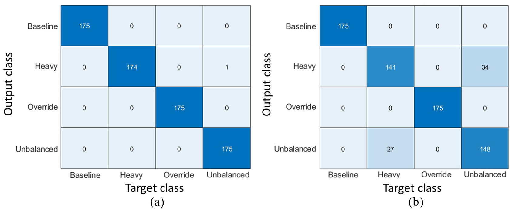
Example confusion matrices summarising the performance of the k-nearest neighbour classification technique when tested on the spindle rotation fingerprint routine: (a) full feature set and (b) reduced feature set.

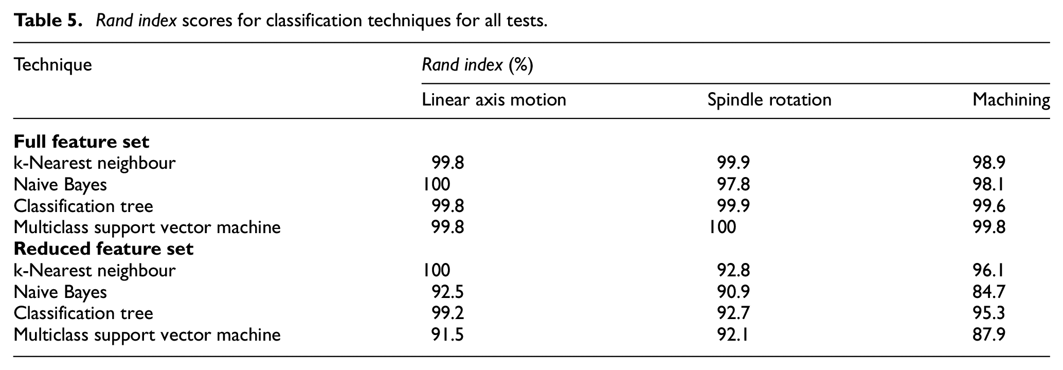
As can be seen in Table 5, all of the classification techniques tested performed well on the full feature sets across all of the routines. There was a slight reduction in performance when using the reduced feature sets. However, considering that the number of features had been reduced from at least 45 down to three, this minor reduction in performance is relatively insignificant.

Table 5.

Rand index scores for classification techniques for all tests.

Technique	Rand index (%)
Technique	Linear axis motion	Spindle rotation	Machining
Full feature set
k-Nearest neighbour	99.8	99.9	98.9
Naive Bayes	100	97.8	98.1
Classification tree	99.8	99.9	99.6
Multiclass support vector machine	99.8	100	99.8
Reduced feature set
k-Nearest neighbour	100	92.8	96.1
Naive Bayes	92.5	90.9	84.7
Classification tree	99.2	92.7	95.3
Multiclass support vector machine	91.5	92.1	87.9

Clustering

The only information supplied to each clustering technique was the number of desired clusters, and the unlabelled feature sets. The results of clustering cannot be visualised as a confusion matrix. However, it was possible to produce graphs illustrating the clustering performance in the three-dimensional feature space, as shown in Figure 11. The graphs presented compare the clustering results from GMM and k-means clustering techniques (Figure 11(b) and (c)) with the actual failure mode categories (Figure 11(a)) from the linear fingerprint routine results.

Figure 11.

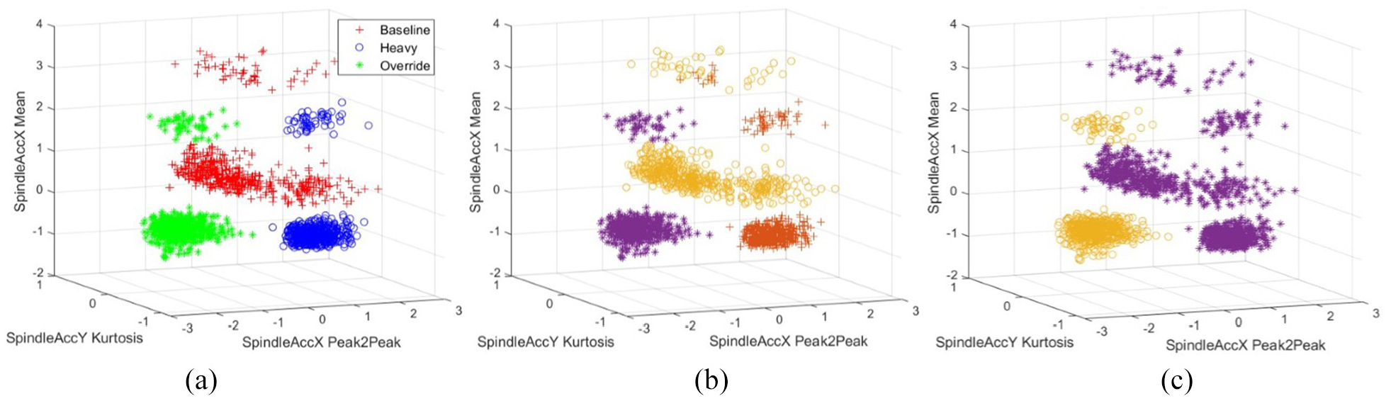
Graphical comparison of (a) the actual categories for the linear fingerprint routine, against the results from: (b) the GMM and (c) the k-means (‘sqeuclidian’ distance metric) clustering techniques. Note that the different markers in (b) and (c) represent the three different clusters.

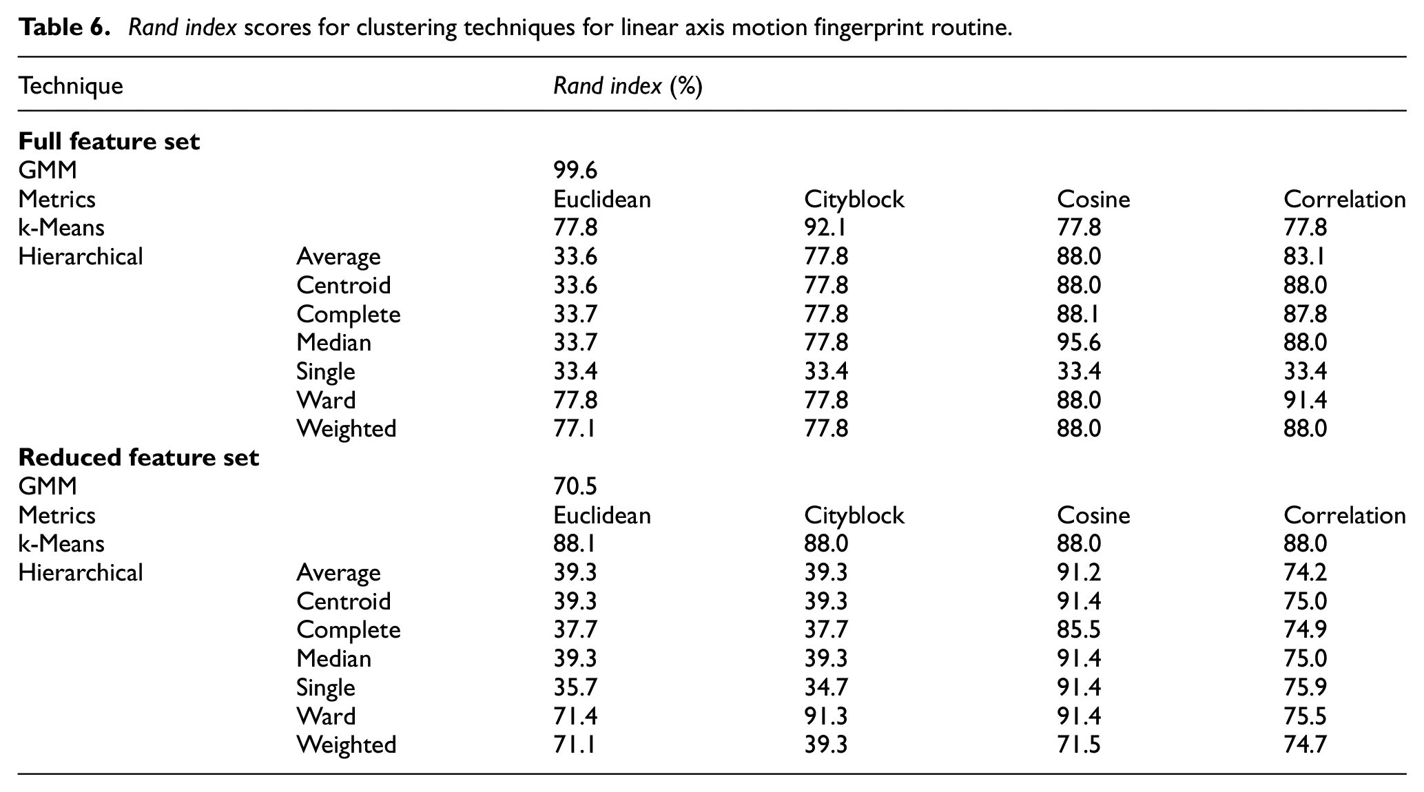
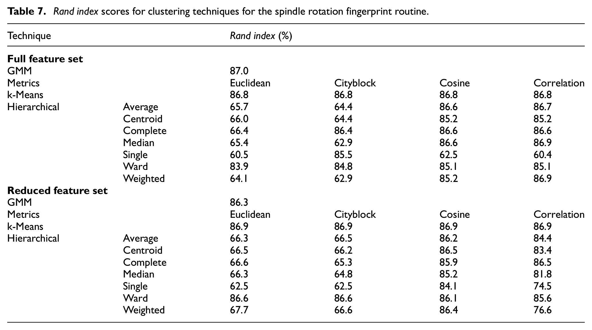
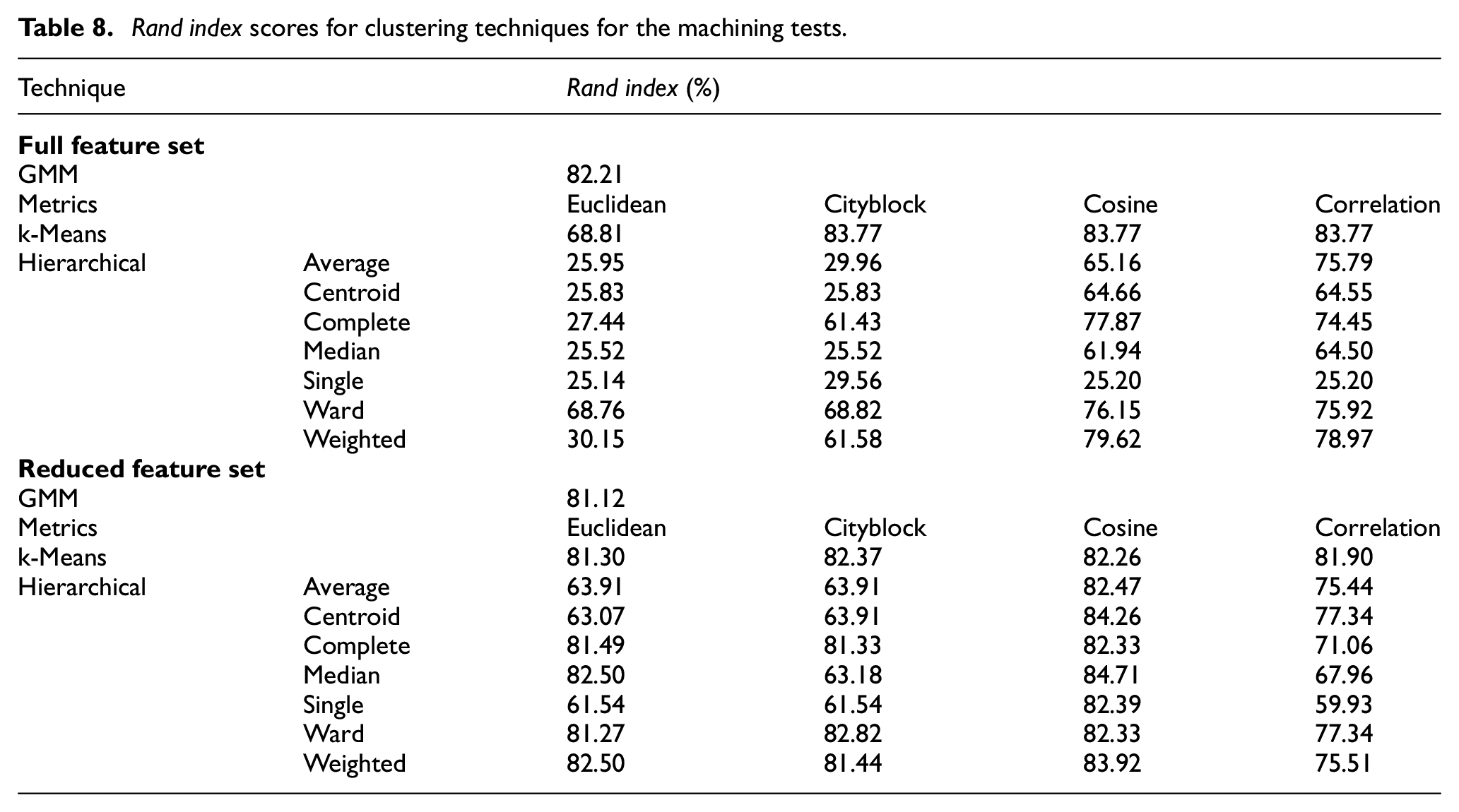
As can be seen, certain techniques, such as the GMM in this case, exhibit a strong correlation to the actual categories (i.e. the results have been split into clusters that accurately match the failure mode categories); whereas others, such as the k-means, perform less well. Tables 6 –8 contain the Rand index scores for all of the techniques, with the various parameters, for both fingerprint routines and the machining tests. It is difficult to identify any trends in performance when switching between the full and reduced feature sets. In general, however, it can be said that the ‘cosine’ distance metric seemed to be the most succesful fork-means and hierarchical techniques; and the GMM also seemed robust throughout all of the tests.

Table 6.

Rand index scores for clustering techniques for linear axis motion fingerprint routine.

Technique		Rand index (%)
Full feature set
GMM		99.6
Metrics		Euclidean	Cityblock	Cosine	Correlation
k-Means		77.8	92.1	77.8	77.8
Hierarchical	Average	33.6	77.8	88.0	83.1
	Centroid	33.6	77.8	88.0	88.0
	Complete	33.7	77.8	88.1	87.8
	Median	33.7	77.8	95.6	88.0
	Single	33.4	33.4	33.4	33.4
	Ward	77.8	77.8	88.0	91.4
	Weighted	77.1	77.8	88.0	88.0
Reduced feature set
GMM		70.5
Metrics		Euclidean	Cityblock	Cosine	Correlation
k-Means		88.1	88.0	88.0	88.0
Hierarchical	Average	39.3	39.3	91.2	74.2
	Centroid	39.3	39.3	91.4	75.0
	Complete	37.7	37.7	85.5	74.9
	Median	39.3	39.3	91.4	75.0
	Single	35.7	34.7	91.4	75.9
	Ward	71.4	91.3	91.4	75.5
	Weighted	71.1	39.3	71.5	74.7

Table 7.

Rand index scores for clustering techniques for the spindle rotation fingerprint routine.

Technique		Rand index (%)
Full feature set
GMM		87.0
Metrics		Euclidean	Cityblock	Cosine	Correlation
k-Means		86.8	86.8	86.8	86.8
Hierarchical	Average	65.7	64.4	86.6	86.7
	Centroid	66.0	64.4	85.2	85.2
	Complete	66.4	86.4	86.6	86.6
	Median	65.4	62.9	86.6	86.9
	Single	60.5	85.5	62.5	60.4
	Ward	83.9	84.8	85.1	85.1
	Weighted	64.1	62.9	85.2	86.9
Reduced feature set
GMM		86.3
Metrics		Euclidean	Cityblock	Cosine	Correlation
k-Means		86.9	86.9	86.9	86.9
Hierarchical	Average	66.3	66.5	86.2	84.4
	Centroid	66.5	66.2	86.5	83.4
	Complete	66.6	65.3	85.9	86.5
	Median	66.3	64.8	85.2	81.8
	Single	62.5	62.5	84.1	74.5
	Ward	86.6	86.6	86.1	85.6
	Weighted	67.7	66.6	86.4	76.6

Table 8.

Rand index scores for clustering techniques for the machining tests.

Technique		Rand index (%)
Full feature set
GMM		82.21
Metrics		Euclidean	Cityblock	Cosine	Correlation
k-Means		68.81	83.77	83.77	83.77
Hierarchical	Average	25.95	29.96	65.16	75.79
	Centroid	25.83	25.83	64.66	64.55
	Complete	27.44	61.43	77.87	74.45
	Median	25.52	25.52	61.94	64.50
	Single	25.14	29.56	25.20	25.20
	Ward	68.76	68.82	76.15	75.92
	Weighted	30.15	61.58	79.62	78.97
Reduced feature set
GMM		81.12
Metrics		Euclidean	Cityblock	Cosine	Correlation
k-Means		81.30	82.37	82.26	81.90
Hierarchical	Average	63.91	63.91	82.47	75.44
	Centroid	63.07	63.91	84.26	77.34
	Complete	81.49	81.33	82.33	71.06
	Median	82.50	63.18	84.71	67.96
	Single	61.54	61.54	82.39	59.93
	Ward	81.27	82.82	82.33	77.34
	Weighted	82.50	81.44	83.92	75.51

Convolutional neural networks

The training, validation and testing procedure for CNNs described in Section 4.2.2 was carried out for both filtered and raw CWTs with the custom-made and pre-trained CNNs. An example of this training and validation process is shown in Figure 12.

Figure 12.

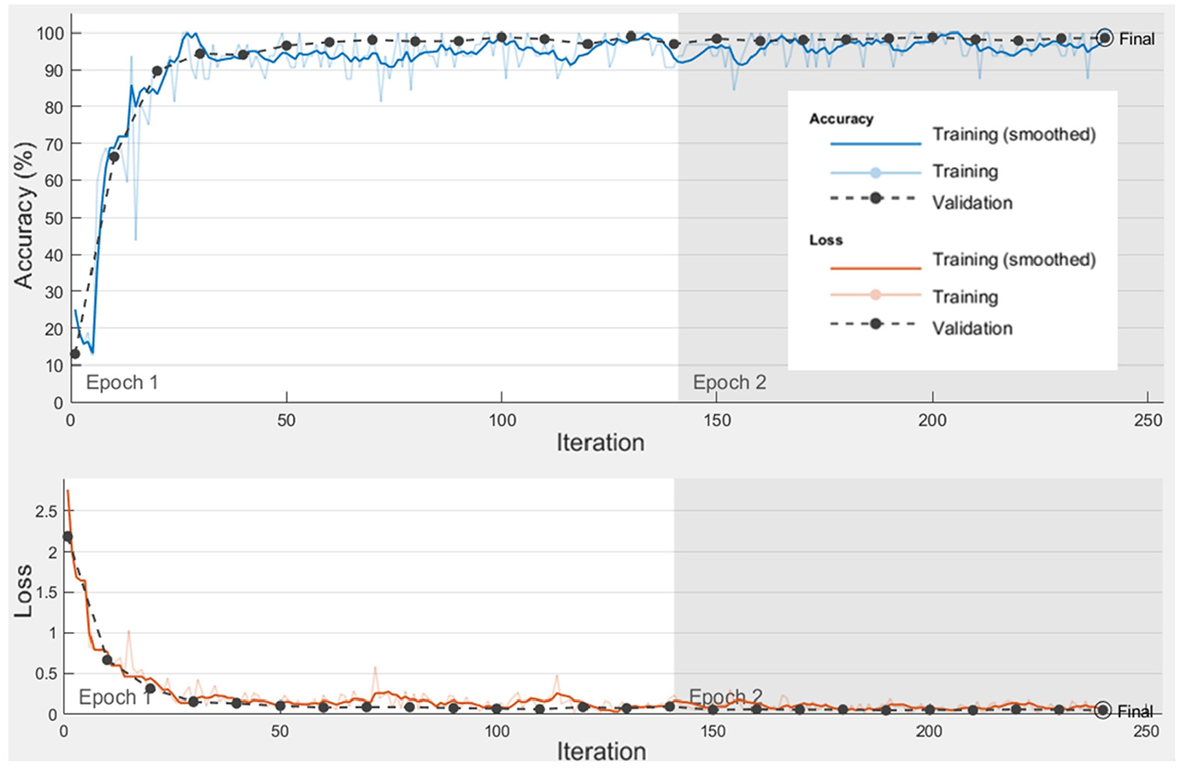
Training progress of the filtered CWTs from the Sensor Plate’s X-axis accelerometer, using the custom-made 2D CNN.

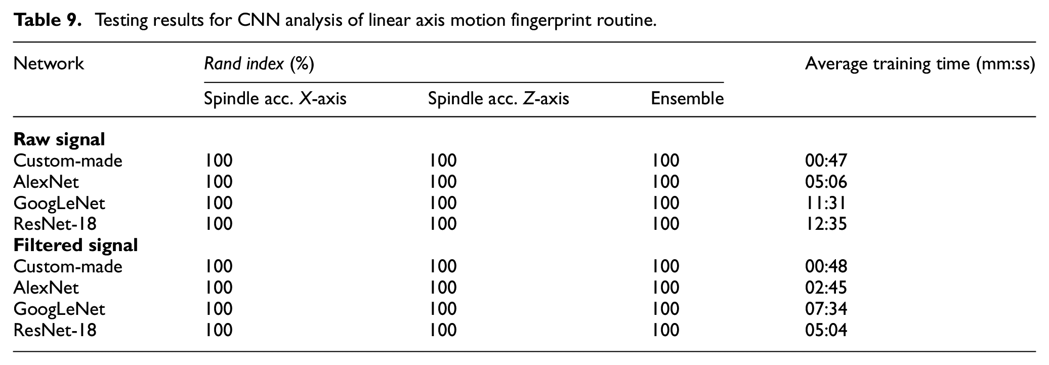
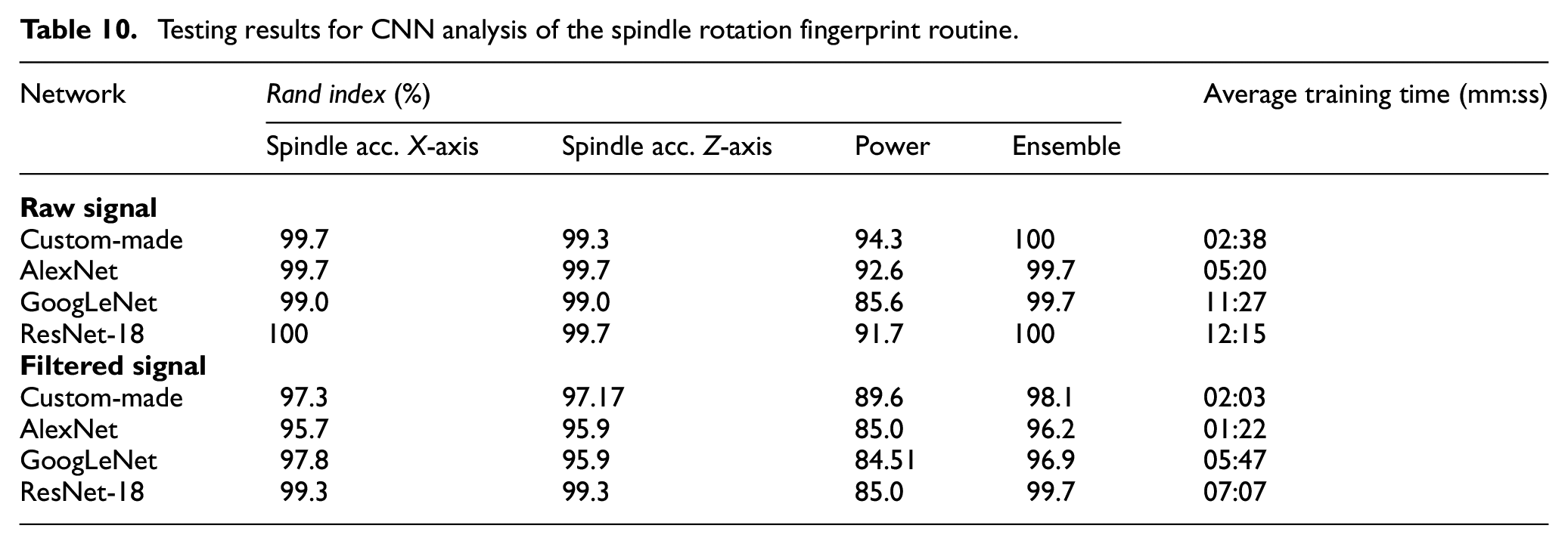
Tables 9–11 show the testing Rand index scores across the CNNs for both fingerprint routine tests and the machining trials respectively. It was identified that standalone CNNs could also be used in conjunction through ‘ensemble learning’. Ensemble learning is the use of multiple learners to provide a single result that is more robust than a learner in isolation. Although relatively complex techniques for combining the outputs of multiple learners have been demonstrated in the literature, such as those proposed by Li et al.²⁶ and Ma et al.²⁷; for this research, a more simplistic approach was opted for. The mean classification scores were calculated from each of the CNNs, and then the maximum of the averaged scores was used to provide the final classification.

Table 9.

Testing results for CNN analysis of linear axis motion fingerprint routine.

Network	Rand index (%)			Average training time (mm:ss)
Network	Spindle acc. X-axis	Spindle acc. Z-axis	Ensemble	Average training time (mm:ss)
Raw signal
Custom-made	100	100	100	00:47
AlexNet	100	100	100	05:06
GoogLeNet	100	100	100	11:31
ResNet-18	100	100	100	12:35
Filtered signal
Custom-made	100	100	100	00:48
AlexNet	100	100	100	02:45
GoogLeNet	100	100	100	07:34
ResNet-18	100	100	100	05:04

Table 10.

Testing results for CNN analysis of the spindle rotation fingerprint routine.

Network	Rand index (%)				Average training time (mm:ss)
Network	Spindle acc. X-axis	Spindle acc. Z-axis	Power	Ensemble	Average training time (mm:ss)
Raw signal
Custom-made	99.7	99.3	94.3	100	02:38
AlexNet	99.7	99.7	92.6	99.7	05:20
GoogLeNet	99.0	99.0	85.6	99.7	11:27
ResNet-18	100	99.7	91.7	100	12:15
Filtered signal
Custom-made	97.3	97.17	89.6	98.1	02:03
AlexNet	95.7	95.9	85.0	96.2	01:22
GoogLeNet	97.8	95.9	84.51	96.9	05:47
ResNet-18	99.3	99.3	85.0	99.7	07:07

Table 11.

Testing results for CNN analysis of the machining tests.

Network	Rand index (%)					Average trainingtime (mm:ss)
Network	Sensor Plateacc. X-axis	Sensor Plateacc. Z-axis	Spindle acc.X-axis	Spindle acc.Z-axis	Ensemble	Average trainingtime (mm:ss)
Raw signal
Custom-made	99.79	95.65	95.25	94.42	100	02:00
AlexNet	98.19	97.81	99.90	93.77	100	03:40
GoogLeNet	96.00	94.45	99.48	93.52	99.28	12:55
ResNet-18	97.07	96.62	99.90	89.12	99.48	07:35
Filtered signals
Custom-made	97.04	99.38	98.48	94.19	100	01:25
AlexNet	98.39	99.79	96.86	94.06	100	02:35
GoogLeNet	99.28	100	97.61	96.26	100	06:35
ResNet-18	99.79	99.69	98.46	94.47	100	07:30

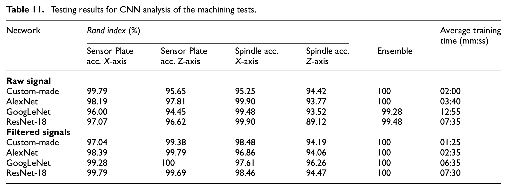
As it can be seen, the Rand index values for the vast majority of the ensemble learning are higher than the standalone networks. This method therefore seems to provide a more robust classification, through a balanced fusion and evaluation of different types of sensors.

It was observed that the significantly simpler custom-made CNNs were able to achieve similar accuracies to that of the pre-trained networks, despite also having generally significantly shorter training times. This could also be attributed to the low complexity of the CWT images and the small number of categories, as they may not require such deep networks. This is supported by the results from the linear fingerprint routine, where each network was able to identify the failure mode correctly with 100% accuracy. This could be indicative of the failure modes being highly distinctive, and so not providing much of a challenge for the networks.

As can be seen in Figure 12, the accuracy and loss converged towards the maximum and minimum values, respectively, relatively quickly. This was the case for most of the other tests, particularly those involving the vibration signals. This may indicate that the number of repeats required to train the CNNs could be significantly less than the number provided in these tests.

It should also be noted that the difference in accuracies achieved by the CNNs when trained on the filtered and raw CWTs is minimal. In the case of the spindle rotation tests, there was in fact a decrease in accuracies overall when using the filtered CWTs. This was unexpected, as the filtering technique makes any changes in the signal far more obvious to the human eye. However, this is obviously not the case for CNNs, meaning that they may perform better when provided the raw, unfiltered signal.

Conclusion

This research developed a machine and process monitoring system by implementing ML techniques for analysis, including clustering, classification and PCA; along with deep learning in the form of CNNs. To enable this, experimental trials were conducted, which included running a fingerprint routine and machining of aluminium blocks under the influence of various simulated failure modes.

In general, the accuracies achieved across all of the techniques tested were promising, with only a small minority not achieving at least mediocre results. A summary of the main findings are provided below:

PCA was used to inform the reduction of a large feature set, whilst retaining variance in the observations. This feature reduction, in some cases by up to 35 times, was found to not have a major impact on the resulting classification/clustering accuracies for most of the classical ML techniques tested.

All of the classification techniques performed well, achieving close to 100% of failure modes/defects correctly classified when utilising the full feature sets. These also remained robust when testing with the reduced feature sets - with all of the techniques remaining above 84% accuracy.

It was difficult to identify particularly successful or unsuccessful clustering techniques, as their performance could vary dramatically depending on which feature set was being analysed. However, GMM seemed to be one of the more consistent techniques for successfully splitting results into clusters that match the actual failure mode/defect categories.

The custom-made CNNs trained in this project appeared to be able to achieve comparable, if not higher, accuracies for classifying failure mode/defect categories than when utilising transfer learning with pre-trained networks; despite having a significantly simpler structure, and therefore shorter training times.

Ensemble learning, when applied to the CNN analysis, has been found to increase the accuracy achieved when compared to using a standalone network in most cases.

The filtering technique defined in previous research¹⁹ seemed to have a smaller impact than had been expected. Although the filtering technique makes changes in the signal more obvious to the human eye, it seems CNNs may benefit from being presented the raw images.

Although the consistent 100% accuracy achieved for the CNN analysis of linear axis motion fingerprint routine may indicate the power of applying such techniques; it may also point to the physical simulation of each failure mode being too distinctive or exaggerated. It is therefore difficult to gauge the real-world performance of the system without being able to test it on real examples of failure modes

With the successes outlined above, there is clearly justification for further development of such techniques in the application to machine tool and process health monitoring. One potential methodology of employing such techniques could be a hybrid system comprised of both classical ML and CNNs. Classification techniques could be used to provide the initial near-/real-time detection of a fault/failure mode; triggering an alarm or even stopping the process to help prevent further damage to the machine tool or component. CNNs could then be used post-event to provide a robust classification of the detected fault to support diagnosis and maintenance activities. Clustering techniques could also be employed in detecting previously unseen/untrained failure modes or defects.

Other research opportunities include testing such a system on more nuanced or less exaggerated failure modes to gauge fidelity; testing of the pre-trained custom-made networks on alternative routines or machine tools through transfer learning to help reduce training samples; and investigations into more comprehensive fingerprint routines and varied machine operations.

Footnotes

Declaration of conflicting interests

The author(s) declared no potential conflicts of interest with respect to the research, authorship, and/or publication of this article.

Funding

The author(s) disclosed receipt of the following financial support for the research, authorship, and/or publication of this article: This work was supported by HVM Catapult funding provided by Innovate UK (project number 160080). The authors would also like to thank Dr Erdem Ozturk for his editorial guidance.

ORCID iDs

James Moore

Jon Stammers

Javier Dominguez-Caballero

References

Teti

Jemielniak

O’Donnell

, et al. Advanced monitoring of machining operations. CIRP Ann - Manuf Technol 2010; 59: 717–739.

MARPOSS Monitoring Solutions GmbH. Tool and process monitoring | Artis Marposs, https://artis.de/eng/ (accessed 27 April 2020).

Nordmann GmbH & Co. KG. NORDMANN Tool Monitoring, http://www.toolmonitoring.com/strategien.html (accessed 27 April 2020).

Sandvik Coromant. CoroPlus® Process Control, https://www.sandvik.coromant.com/en-gb/products/coroplus-processcontrol/Pages/default.aspx (accessed 27 April 2020).

Ben Ali

Saidi

Harrath

, et al. Online automatic diagnosis of wind turbine bearings progressive degradations under real experimental conditions based on unsupervised machine learning. Appl Acoust. Epub ahead of print 2018. DOI: 10.1016/j.apacoust.2017.11.021.

D’Emilia

Gaspari

Hohwieler

, et al. Improvement of defect detectability in machine tools using sensor-based condition monitoring applications. Procedia CIRP 2018; 67: 325–331.

Uhlmann

Laghmouchi

Hohwieler

, et al. Condition monitoring in the cloud. Procedia CIRP 2015; 38: 53–57.

Nam

Kim

, et al. Development of a health monitoring and diagnosis framework for fused deposition modeling process based on a machine learning algorithm. Proc Inst Mech Eng Part B J Eng Manuf 2020; 234: 324–332.

Kaya

Oysu

Ertunc

, et al. A support vector machine-based online tool condition monitoring for milling using sensor fusion and a genetic algorithm. Proc Inst Mech Eng Part B J Eng Manuf 2012; 226: 1808–1818.

10.

Zhao

Mei

, et al. Thermal error compensation based on genetic algorithm and artificial neural network of the shaft in the high-speed spindle system. Proc Inst Mech Eng Part B J Eng Manuf 2017; 231: 753–767.

11.

Segreto

Simeone

Teti

Principal component analysis for feature extraction and NN pattern recognition in sensor monitoring of chip form during turning. CIRP J Manuf Sci Technol 2014; 7: 202–209.

12.

Sevilla-Camacho

Robles-Ocampo

Jauregui-Correa

, et al. FPGA-based reconfigurable system for tool condition monitoring in high-speed machining process. Measurement 2015; 64: 81–88.

13.

Wang

Zhuang

Duan

, et al. A multi-scale convolution neural network for featureless fault diagnosis. In: International Symposium on Flexible Automation, ISFA 2016. pp. 65–70. Cleveland, OH: IEEE.

14.

Wang

Ananya, Yan

, et al. Virtualization and deep recognition for system fault classification. J Manuf Syst 2017; 44: 310–316.

15.

Guo

Zhou

An intelligent monitoring system of grinding wheel wear based on two-stage feature selection and long short-term memory network. Proc Inst Mech Eng Part B J Eng Manuf 2019; 233: 2436–2446.

16.

Wang

Niu

Sun

Chatter identification in thin-wall milling using an adaptive variational mode decomposition method combined with the decision tree model. Proc Inst Mech Eng Part B J Eng Manuf 2020; 095440542093370.

17.

Tiwari

Vergidis

Lloyd

, et al. Automated inspection using database technology within the aerospace industry. Proc Inst Mech Eng Part B J Eng Manuf 2008; 222: 175–183.

18.

Psarommatis

May

Dreyfus

, et al. Zero defect manufacturing: state-of-the-art review, shortcomings and future directions in research. Int J Prod Res 2020; 58: 1–17.

19.

Dominguez-caballero

Stammers

Moore

. Development and testing of a combined machine and process health monitoring system. In: 7th CIRP Global Web Conference - Towards shifted production value stream patterns through inference of data, models, and technology, Berlin, 2019. vol 86, pp. 20–25. Elsevier B.V.

20.

British Standards Institution. BS ISO 10791-7:2014 - Test conditions for machining centres - Part 7: Accuracy of finished test pieces. 2014; 36.

21.

Saidi

Ben Ali

Bechhoefer

, et al. Wind turbine high-speed shaft bearings health prognosis through a spectral Kurtosis-derived indices and SVR. Appl Acoust. Epub ahead of print 2017. DOI: 10.1016/j.apacoust.2017.01.005.

22.

Rand

WM.

Objective criteria for the evaluation of clustering methods. J Am Stat Assoc 1971; 66: 846.

23.

Wold

Esbensen

Geladi

Principal component analysis. Chemom Intell Lab Syst 1987; 2: 37–52.

24.

Hoang

D-T

Kang

H-J.

Rolling element bearing fault diagnosis using convolutional neural network and vibration image. Cogn Syst Res 2019; 53: 42–50.

25.

Szegedy

Liu

Jia

, et al. Going deeper with convolutions. In: Proceedings of the IEEE Computer Society Conference on Computer Vision and Pattern Recognition. 2015, pp. 1–9. Boston, MA: IEEE Computer Society.

26.

Jiang

Niu

, et al. An enhanced selective ensemble deep learning method for rolling bearing fault diagnosis with beetle antennae search algorithm. Mech Syst Signal Process 2020; 142: 106752.

27.

Chu

Ensemble deep learning-based fault diagnosis of rotor bearing systems. Comput Ind 2019; 105: 143–152.

The application of machine learning to sensor signals for machine tool and process health assessment

Abstract

Keywords

Introduction

Experimental setup

Experimental method

Failure mode and defect physical simulation

Analysis methodology

Data processing

Feature extraction

Continuous wavelet transform and filtering

Image composition and resizing

Machine learning techniques

Classical machine learning

Convolutional neural networks structures and parameters

Results and discussion

Classical machine learning

Principal component analysis and feature reduction

Classification

Clustering

Convolutional neural networks

Conclusion

Footnotes

Declaration of conflicting interests

Funding

ORCID iDs

References